ANABIOPLUS: A NEW PACKAGE FOR PARAMETER ESTIMATION AND SIMULATION OF BIOPROCESSES

Vol. 34, No. 04, pp. 1065 – 1082, October – December, 2017 dx.doi.org/10.1590/0104-6632.20170344s20150673

* To whom correspondence should be addressed

ANABIOPLUS: A NEW PACKAGE FOR

PARAMETER ESTIMATION AND SIMULATION OF

BIOPROCESSES

C.M. Oliveira

_{, C.D.F. Jesus}

_{, L.V.S. Ceneviva}

_{, F.H. Silva}

_{, A.J.G. Cruz}

_,

C.B.B.Costa

_{and A.C. Badino}

_*

1_{PPGEQ/UFSCar – Chemical Engineering Graduate Program, Federal University of São Carlos, Brazil} 2_{Brazilian Bioethanol Science and Technology Laboratory, Brazil}

3_{Department of Chemical Engineering, Federal University of São Carlos} Rodovia Washington Luiz Km 235, 13565-905, São Carlos, São Paulo, Brazil

4_{Department of Chemical Engineering, State University of Maringá, Brazil}

*Corresponding author: badinojr@ufscar.br; Phone: +55 16 3351-8001, Fax: +55 16 3351-8266

(Submitted: October 23, 2015; Revised: June 10, 2016; Accepted: June 12, 2016)

Abstract – A very important step in the study of bioprocesses is the modeling and simulation of bioreactors. This paper presents the AnaBioPlus software package, which was developed for teaching and research purposes concerning the analysis of bioreactors. The package consists of two programs: OptimusFerm and SimulaFerm. OptimusFerm allows the analysis of experimental batch cultivation data sets in order to estimate parameters of kinetic models by means of

a differential evolution method. SimulaFerm performs simulations obtaining values of cell growth, product formation,

and limiting substrate consumption for batch, fed-batch and continuous cultivations. Thirty-two kinetic models of cell growth are available in OptimusFerm and SimulaFerm. Two case studies are described in order to illustrate the use of AnaBioPlus. The results show that AnaBioPlus is a very useful tool for the analysis of bioprocesses. Furthermore, it presents a user-friendly graphical interface and is freely available to users, in both English and Portuguese versions.

Keywords: Free software, bioprocess, kinetic modeling, parameter estimation, simulation.

INTRODUCTION

Bioprocessesare present in many industrial processes, including the production of foods, antibiotics, amino acids, organic acids, and ethanol. They are also used in wastewater treatment. Bioprocess reactions are often carried out in bioreactors, involving consumption of substrate, formation of product, and growth of the microorganism responsible for the bioprocess. Therefore, modeling of bioreactors is an important stage in the evaluation of biochemical processes.

In bioprocess modeling, mathematical equations are used to describe the specific growth rate of biomass, which is used in mass balance equations. Many mathematical

models are available in the literature to describe cell growth rates, with and without substrate, as well as product and/or cell inhibition (Monod, 1942; Moser, 1958; Contois, 1959; Aiba et al., 1968; Andrews, 1968; Levenspiel, 1980; Hoppe and Hansford, 1982; Lee et al., 1983; Wu et al., 1988), and can be used in simulation modeling of bioprocesses.

Several software packages have been developed for simulation of biochemical processes. OptFerm is a computational platform for the simulation and optimization of bioprocesses,where the objective is to calculate the best concentration of nutrients to initiate the fed-batch bioprocess. Moreover, the user can perform an estimation of kinetic and yield parameters in order to obtain the best

of Chemical

possible model setup (Rocha et al., 2009). BioMASS is a simulator that allows users to specify the feed, bioreactor type, operating conditions, and cell growth kinetic model. The program then predicts substrate, product, and biomass concentrations over a given period of bioreactor operation (Phan-Thien, 2011). KINSOLVER is a simulator that uses a representation of the chemical reactions as the input file, instead of a system of differential equations. Concentrations of participating species are specified at the initial time, and the system is solved for concentrations at a final time. Kinetic parameters and initial conditions are all part of the input file (Aleman-Meza, 2011). KINSIM is software for simulation of the progress of kinetic curves, where the user inserts a representation of a chemical reaction scheme using conventional chemical format, after which differential equations representing the mechanism are generated and a direct numerical integration is performed. KINSIM software can be used to simulate any number of reaction mechanisms (Barshop et al., 1983). Commercial software can also be used for the simulation of biochemical processes, employing packages such as Aspen Plus®_{orSuperPro Designer}®_{. EMSO (Environment} for Modeling, Simulation, and Optimization) software is an equation-oriented process simulator for modeling dynamic or steady-state processes, distributed at no cost for academic purposes. The software has its own modeling language, and new models can be developed by the users (Soares and Secchi, 2003). The simulator platform provides a tool for parameter estimation. However, the license costs of the Aspen Plus and SuperPro Designer software packages and the need for previous knowledge in using the EMSO software are important considerations. When the focus is on estimating the parameters of kinetic models, programs that make use of numerical integration of rate equations are available, such as FITSIM (Zimmerle and Frieden, 1989), besides commercial software packages that have tools for solving optimization problems, such as Matlab®_{, Scilab}®_{, MathCad}®_{, Berkeley Madonna}®_{, and} Scientist®_.

The Global Kinetic Explorer (Johnson, 2009), COPASI (Hoops, 2006), KINFITSIM (Svir et al., 2002), and GEPASI (Mendes, 1983)tools simulate biochemical reactions and estimate reaction kinetics parameters. The commercial Global Kinetic Explorer program is available as a professional version and as a free student version that has limited resources. COPASI is a successor to GEPASI and is free for non-commercial use. The KINFITSIM commercial software is available at a discount for academic purposes. Several other important software tools are being developed for use in cell biology, such as CELL (Tomita et al., 1999), Virtual Cell (Loew and Schaff, 2001), E-MCell (Stiles and Bartol, 2001), StochSim (Novère and Shimizu, 2001), STOCKS (Kierzek, 2002), BioSPICE(Garvey, 2003), and ETA (Murphy and Young, 2013).

As can be seen, the literature offers various software options with different characteristics. However, no

non-commercial software package is available that estimates kinetic parameters of cell growth models, while at the same time simulating different bioprocesses by means of a user-friendly graphical interface. The present work therefore presents AnaBioPlus, a software package for analysis of bioreactors. AnaBioPlus contains two software modules: OptimusFerm and SimulaFerm. These free and flexible tools can be easily used by persons with minimal training. OptimusFerm is software for estimation of the parameters of cell growth kinetic models, and allows the analysis of more than one batch cultivation experimental data set. Once the kinetic model has been chosen, its parameters are estimated by means of the differential evolution method. The values of the estimated parameters are then displayed, for a confidence interval of 95%, together with a graphical representation of the experimental points and the fitted curve.

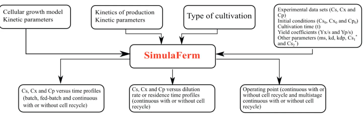
SimulaFerm is a simulator of bioprocesses in which the user can specify the cultivation mode (batch, fed-batch, continuous without and with recycle, and with tanks in series), the initial and operating conditions, and the cell growth kinetic model. Simulation is then performed of the behavior of the substrate, cell, and product concentrations as a function of time under transient cultivation conditions or at steady state in continuous cultivation. The software provides help topics concerning its operation, bioprocess kinetics, and types of cultivation, including the corresponding equations. The user can simulate the same process under different cultivation conditions and overlap the curves predicting substrate, biomass, and product concentrations. Experimental data can also be added. AnaBioPlus installation is simple, and both software modules have thirty-two kinetic models of cell growth available.

PRESENTATION OF ANABIOPLUS

AnaBioPlus version 1.0 was developed with the objective of helping researchers and students in the analysis of bioreactors. It is a non-commercial software package consisting of two programs: OptimusFerm and SimulaFerm. OptimusFerm is software for estimating kinetic parameters of cell growth kinetic models, and SimulaFerm is a simulator for bioprocesses. The package has a user-friendly interface, which provides the user with easy access to program resources. AnaBioPlus has some routines (executable, *.dll) in Fortran®_{. The software was} developed using Microsoft Visual Basic® _{and is available} in Portuguese and English versions.

OptimusFerm

that maximize (or minimize) one or more objective functions, with or without constraints. In this work, the problem to be solved is a nonlinear optimization, where the objective function (Φ) is minimized (Eq. 1). The constraints (Eq. 2) are the upper and lower bounds of the parameters to be estimated, b_i, which are defined by the user. The experimental and calculated concentrations of substrate,

biomass, and product are normalized in the objective function (Φ) in order to avoid excessiveweightings in the data set. The experimental and calculated values of each dependent variable are scaled using the maximum value found for that variable in the data set. When multiple batch runs are used, the maximum value of each variable is searched among the data set of each batch.













2

1 2

1

min







  















S

x

x

x

x

x

x

i , 1,...,

sup

inf _{  }

Many approaches can be used for parameter estimation, ranging from classical deterministic methods, such as Levenberg-Marquardt (LM), to newer methods based on ecological and biological behavior, such as evolutionary algorithms (EAs). The latter have many advantages over conventional nonlinear programming techniques, including no requirement for the gradients of the cost or constraint functions, simple implementation, and less chance of becoming trapped in a local minimum (Nelles, 2001; Long et al., 2013).

The evolutionary algorithm class contains several families of methods, which have different advantages and disadvantages. In developing OptimusFerm, a differential evolution (DE) algorithm was used. Differential evolution is a heuristic method for minimizing possible nonlinear

and non-differentiable continuous space functions. Evolutionary algorithms have proven effective in solving many engineering optimization problems and have the advantage of being less susceptible to local minima. The DE algorithm has many useful characteristics, such aseasy implementation, requirement for only a few control variables, and robustness (Nelles, 2001). Furthermore, the DE algorithm does not require parameter initialization, in contrast to derivative methods (such as the LM method). In derivative methods, if an initial set of bad parameter values is set, the method could diverge. Moreover, most complex real-world applications can be solved with this method (Storn and Price, 1997).

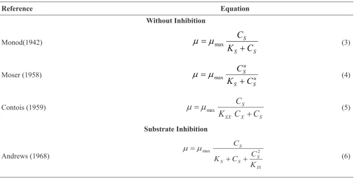
OptimusFerm contains 32 non-segregated and unstructured kinetic models of cell growth (µ). These models are divided into different categories: no inhibition, substrate inhibition, product inhibition, cellular inhibition, and hybrid inhibition. Table 1 shows some of the models present in the software.

(1)

(2)

Table 1. Cell growth kinetic models.

Reference Equation Without Inhibition Monod(1942) S S S

C

K

C

+

=

µ

µ

Moser (1958) _u

S S u S

C

K

C

+

=

µ

µ

C

C

K

C







The 4th _{order Runge-Kutta method is used to solve} the set of ordinary differential equations that describe the mass balance for biomass, substrate, and product in the operationalmode of the bioreactor. Five different types of cultivation are available in the SimulaFerm software (batch, fed-batch, continuous without cell recycle, continuous with external cell recycle, and continuous with internal cell recycle). As an example, a set of mass balances for batch cultivationis described by Eqs. 12-14.

D X X r r dt

dC _{ }

S S

r

dt

dC

_

_

dC _{ }

In Eqs.12-14, the terms r_X, r_D, r_S, r_P, and r_DP, are the rates of cell growth, cell death, substrate consumption, product formation, and product degradation, respectively (g.L-1_.h-1_). These reaction rates are given in Eqs. 15-19. Substrate

consumption is represented by three terms that account for cell growth, product formation, and cell maintenance (Eq. 17).Product formation can be not associated with growth, partially associated with growth,or both(Eq. 18). C_X, C_S, and C_P are the cell, substrate, and product concentrations, respectively (g.L-1_).

X

X

C

r

=

µ

⋅

X d

D

k

C

r

=

⋅

Sm SP SX

S

r

r

r

r







Cx

β

Cx

μ

α

r











P dp

DP

k

C

r





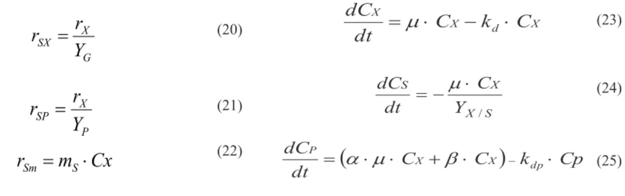
The rates of substrate consumption for biomass production or for cell growth (r_SX), the rate of consumption of substrate for product formation (r_SP), and the rate of consumption of substrate for cell maintenance (r_Sm) are described by Eqs. 20-22.

Reference Equation

Wu et al. (1988) v

IS S S S S S

K

C

C

C

K

C













+

+

=

µ

µ

(7)

Product Inhibition

Hoppe and Hansford (1982)

P IP IP S S S

C

K

K

C

K

C

+

+

=

µ

µ

Aiba et al. (1968) max ( )

P IPC K S S S

_e

C

K

C

+

=

µ

µ

=

µ

µ

Cellular Inhibition

Lee et al. (1983)

m X X S S S

C

C

C

K

C













−

+

=

µ

1

µ

Table 1. Cont.

G X SX

_Y

r

r



P X SP

_Y

r

r



Cx

m

r





In Eqs.20 and 21, Y_G and Y_P are, respectively, thestoichiometric yield coefficient from substrate to cells, also known as the true cell yield coefficient, and the stoichiometric yield coefficient from substrate to product, also known as the true product yield coefficient. The term m_s (Eq. 22) is the maintenance energy coefficient (h-1_).

In practice, it is difficult to determine the exact amount of substrate consumed exclusively for cell growth (Y_G) or product formation (Y_P). Therefore, in mass balances it is usual to express all the substrate consumption by global yield coefficients (Y_X/S and Y_P/S), which are easier to determine experimentally.

The SimulaFerm software allows simulationsto be performed using these two approaches. If the global yield coefficients are used, the mass balances for cells, substrate, and product in batch mode operation are described by Eqs. 23-25. If the global yield coefficients are used, the program calculates the value ofthe α coefficient. However, the β parameter should be provided by the user. However, the β parameter should be provided by the user. If the true cell coefficients are used (Y_G andY_P), the user needs to provide the values of m_s and the α coefficient. The values of the k_d and k_dp coefficients are also provided by the user.

X d X X

C

k

C

dt

dC











S X

X S

Y C dt

dC

/  









dt dC

dp X X

P

 

  









It is possible to input more than one experimental data and cultivation conditions set in OptimusFerm. A very useful tool in any program, which is also present in OptimusFerm and SimulaFerm, is the option to save and open files. A convenient resource for beginners in the use of OptimusFerm is the help file, which contains topics concerning the theory of the differential evolution method and the software resources, as well as instructions on how to use the software for the first time.

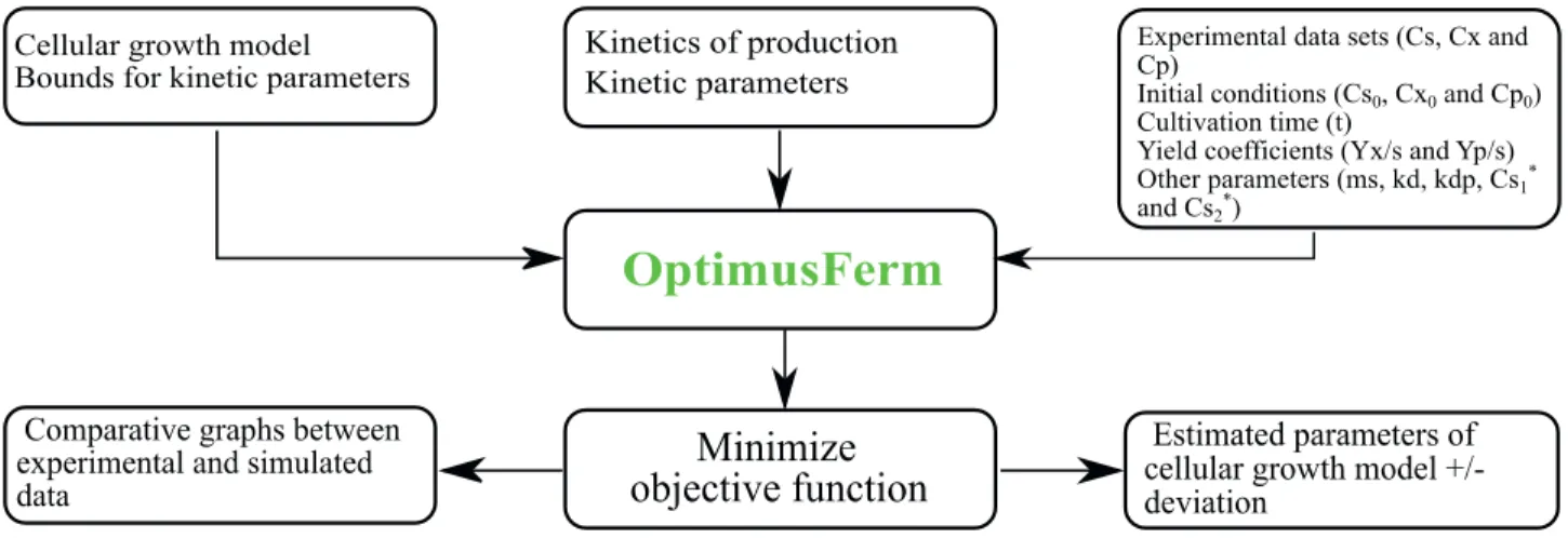
Estimation of kinetic parameters is performed in batch mode, which is the simplest cultivation method. The confidence interval for each estimated parameter is calculated after the convergence of the DE algorithm, taking into account the model chosen, the degree of freedom of the system and the Jacobian matrix, calculated numerically using finite differences. Good descriptions of the theory of parameter estimation for non-linear model scan be found inHimmelblau (1970), Bard (1974), and Nelles (2001).However, simulations can be performed in SimulaFerm with different cultivation conditions, using the cell growth kinetic model parameters previously estimated in OptimusFerm. Fig. 1 shows the OptimusFerm splash screen. Fig. 2 illustrates the flow of information throughout the OptimusFerm software.

Figure 1. OptimusFerm splash screen.

(20)

(21)

(22)

(23)

(24)

SimulaFerm

SimulaFerm version 1.0 is free software for the simulation of bioprocesses by means of mass balances of substrate, cells, and product over time in biochemical reactors under transient cultivation conditions (batch, fed-batch, and transient continuous) and at steady state in continuous cultivation. There are two previous Portuguese versions of SimulaFerm, called AnaBio versions 1.0 and 2.0 (Silva et al., 2003, 2005). The version presented in this paper has improvements in layout and source code and adds new graphical features, and for these reasons the name of the software has been changed to SimulaFerm. The package was named AnaBioPlus to differentiate it from the older AnaBio simulator.

SimulaFerm performs bioreactor simulations, obtaining curves forcell growth, product formation, and limiting substrate consumption. These are presented as a function of time (for cultures operated under transient conditions), and as a function of dilution rate or residence time (for continuous cultivations operated at steady state).

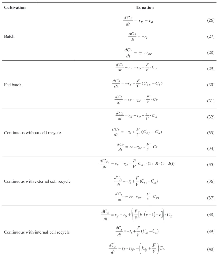
Users can choose among seven different types of bioreactor configuration, such as batch, fed-batch, continuous without recycle, continuous with external cell recycle, continuous with internal cell recycle, multistage continuous without cell recycle, and multistage continuous with cell recycle. Cultures in batch and fed-batch modes are analyzed in the transient state (graphs of concentration versus time). Continuous cultures with or without cell recycle may be analyzed in the transient state (graphs of concentration versus time) or in steady state (graphs of concentration versus dilution rate or residence time), and the user can view the operating points in steady state. Multistage cultivations with or without recycle allow the user to view the operating points in steady state for three tanks connected in series. The 4th_{order Runge-Kutta} method is used to solve the set of ordinary differential equations, and the Newton-Raphson method is used to

solve algebraic equations. Table 2 shows mass balances for substrate, biomass, and product in different bioreactor configurations provided in SimulaFerm. Fig. 3 shows the SimulaFerm splash screen. Fig. 4 illustrates the flow of information throughout the SimulaFerm software.

Thirty-two cell growth kinetic models are available, some of which are shown in Table 1. The user can choose among product formation types: product formation associated with cell growth; product formation not associated with cell growth; and product formation partially associated with cell growth. The program has operating conditions available with or without cell maintenance, cell death, and product degradation.

SimulaFerm has the option of including experimental points along with the simulated profiles for batch and fed-batch configurations. An additional feature is the analysis of cell growth models, in which the program allows animation of the curve of μ versus CS when kinetic parameters of the cell growth model vary (such as μmax and K_S for the Monod model).This tool is of great importance, especially for teaching purposes.

CASE STUDIES

To illustrate the use of OptimusFerm and SimulaFerm, two examples are presentedthat involve the estimation of kinetic parameters and simulation of bioprocesses.

Parameter estimation using OptimusFerm (Case Study 1)

Table 2. Cultivation equations. Cultivation Equation Batch D X X r r dt

dC _{  (26)}

S S

r dt dC _

(27) DP P P r r dt dC   (28) Fed batch X D X X C V F r r dt

dC _{   }

(29)

) ( Sf S S S C C V F r dt

dC _{  }

(30) P DP p P C V F r r dt dC     (31)

Continuous without cell recycle

X D X X C V F r r dt

dC _{   }

(32)

) ( Sf S S S C C V F r dt

dC _{  }

(33) P DP P P C V F r r dt

dC _{ }

 

(34)

Continuous with external cell recycle

)) 1 ( 1 ( 1

1 _{C R B}

V F r r dt dC X D X

X       

(35)

) ( _{0 1}

1

S S S

S _{C C}

V F r dt dC     (36) 1 1 P DP P P C V F r r dt dC     (37)

Continuous with internal cell recycle

 





D X

X _{h c c C}

V F r r dt dC        _{  }  

 1 (38)

) ( _{S0 S} S

S _{C C}

V F r dt dC     (39) P dp DP p P _C V F k r r dt dC       _ 

Cultivation Equation

Multistage continuous without recycle Tank 1 1 1 1 1 X D X X _C V F r r dt dC     (41) 1 1 1 1 S S S C V F r dt dC     ₍₄₂₎ 1 1 1 1 P P P C V F r dt dC    ₍₄₃₎ Tank n )

(  ₁

 

 Xn Dn Xn X_n n X C C V F r r dt dC (44) ) (  _1 



 _{Sn Sn Sn}

Sn _{C C}

V F r dt dC (45)





DPn Pn n P C C V F r r dt dC  

  _1

(46)

Multistage continuous with cell recycle Tank 1   1 1 1 1

1 3 1 1

V C F R V C B F R r r dt

dC X X

D X

X _{  }    _   

(47) 1 1 1 1 3 0 1

1 ( 1)

V C F R V C F R V C F r dt

dC S S S

S

S   

        (48) 1 1 1 3 1 1

1

(

1

)

V

C

F

R

V

C

F

R

r

r

dt

dC

DP P

P

_

_

_





_







(49)

Tank n

)

(  _1

 

 _{Xn Dn Xn Xn}

n X C C V F r r dt dC (50)

)

(

)

1

(











Sn

_R

_C

_C

V

F

r

dt

dC





DPn Pn n P C C R V F r r dt dC    

 ( 1) _1 (52)

Figure 3. SimulaFerm splash screen.

(clavulanic acid) was not associated with cell growth. Baptista-Neto et al. (2000) used the Monod model to describe the bioprocess. The specific growth rate is given by Eq. 3 (Table 1), in which m_max is the maximum specific growth rate (h-1_{) and K}

S is the saturation constant of the Monod model (g.L-1_).

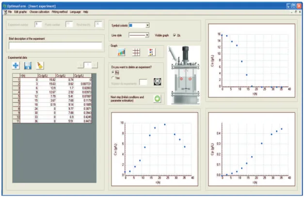
When starting the program, the window “Insert experiment” will open and the user can add the experimental data of the batch cultivation. Fig. 5 shows a window with the experimental substrate, biomass, and product concentration data, as a function of time, as presented by Baptista-Neto et al. (2000). In this example, only one experimental data set was used, but it is possible to input additional data sets. OptimusFerm has a variety of graphical resources available, including color for the markers of the experimental data, line style for the fitted curve, copy and save the graph, and remove or insert gridlines and legend.

Each experiment added must be saved, or it is not used in the estimation. The option “visible graph” may be selected or not, but if it is not selected, the graphs of the experiment will not be exhibited.

The graphs can be enlarged by double clicking on them or by right clicking and selecting Zoom. Fig. 6 shows the window that then opens with the enlarged graph, where it is possible to insert a title, add or remove the legend and the grid lines, delimit the time interval, copy, save, and print the graph.

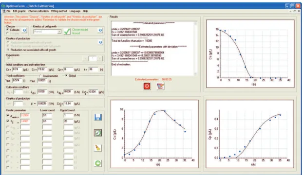
The next step consists of inserting the cultivation conditions of each experiment. Fig. 7 shows a screen capture of the “Batch Cultivation” window for the problem studied. To choose the parameters to be estimated, it is necessary to select them in the field “Kinetic parameters”, add values to start the algorithm, and fill in their respective upper

and lower bounds. In this example, m_max and K_S were the estimated parameters of the Monod model (Eq. 3, Table 1). The experimental data and cultivation conditions can be saved in files with extension “*.abr”, using the menus “File/ Save/Experiments” and “File/Save/Cultivation conditions/ Batch”, respectively. They can then be opened whenever necessary.

In the field “Choose” (Fig. 7), the user can select the option “Estimate”, which estimates the parameters of the kinetic model, or select the option “Simulate”, if the user wants to simulate the process with manually inputted parameters. The sum of squared deviations and the estimated parameters are presented in the “Results” field (Fig. 7).It is possible to stop the estimationby clicking the red button below the Results field. When the estimation is complete, the user can generate a report with cultivation conditions, estimated parameters, and graphs with the experimental data and fitted curves. It is also possible to export the fitted substrate, biomass, and product concentration data using the menu “File/Export/Data (Clipboard)”. This enables graphs to be constructed using external software.

Visual inspection of the fitted curves for the substrate, cell, and product concentrations using the differential evolution method (Fig.7) showed that the parameter estimation could be considered of good quality. This was corroborated by the low values of the sums of squared deviations. The estimated parameter values and confidence intervals were m_max=0.2056±0.0006 h-1 _{and K}

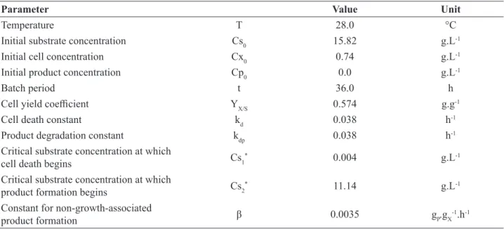
S=3.49±0.29 g.L-1_{. The estimated parameters were within the range of} values found in the literature (Baptista-Neto et al., 2000). The user should pay attention to the standard deviation of the estimated parameters (at 95% confidence interval), because it can be so wide that it includes values outside the limits informed by the user, or be in a range in Table 3. Bioprocess conditions and estimated parameters obtained by Baptista-Neto et al. (2000)(Case Study 1)

Parameter Value Unit

Temperature T 28.0 °C

Initial substrate concentration Cs₀ 15.82 g.L-1

Initial cell concentration Cx₀ 0.74 g.L-1

Initial product concentration Cp₀ 0.0 g.L-1

Batch period t 36.0 h

Cell yield coefficient Y_X/S 0.574 g.g-1

Cell death constant k_d 0.038 h-1

Product degradation constant k_dp 0.038 h-1

Critical substrate concentration at which

cell death begins Cs1

* _{0.004 g.L}-1

Critical substrate concentration at which

product formation begins Cs2

* _{11.14 g.L}-1

Constant for non-growth-associated

product formation β 0.0035 gP.gX

Figure 5. Window to add experimental data for parameter estimation in OptimusFerm (Case Study 1)

Figure 7. Window to insert cultivation conditions, with curves fitted by the Monod model (Case Study 1)

which the parameter value makes no physical sense. The computational time for the parameters estimation was only 7 seconds, for a population of 20 individuals and 200 iterations (Pentium Dual Core 1.73 GHz).

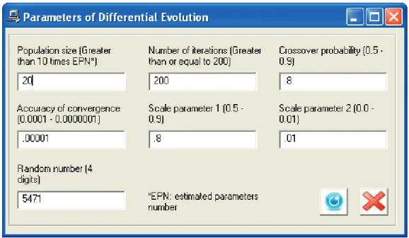
The differential evolution method has control parameters that affect the performance of the algorithm. Some of these parameters, such as the population size and crossover probability, can be modified by the user in order to try to improve the estimation. In OptimusFerm, there are default values for these parameters. To change them, the user must access the menu “Fitting method” or use the shortcut Ctrl+M (Fig. 8). However, alteration of these values by the user should be performed with caution and with prior knowledge. There are some studies in the literature where self-adaptation of the parameters of the differential evolution algorithm is described (Ghosh et al., 2011; Pan et al., 2011), but as this is beyond the scope of the present work, the ranges of these values were only suggested and default values were assigned in accordance with the literature. For the estimation of kinetic parameters presented in this case study, the control parameters were not changed.

A convenient resource for beginners of OptimusFerm is the help file, which contains topics concerning the theory of the differential evolution method and the software resources, as well as instructions on how to use the software. The help file is available from the “Help/Help topics”menu. It is important to mention that the software does not handle the problem of ill-conditioned parameters.

The user must be aware of this problem.

Simulation using SimulaFerm (Case Study 2)

This second case study concerns the bioprocessdescribed by Badino and Hokka (1999) for ethanol production. Table 4 presents the cultivation conditions for this problem. The cell and product yield coefficients (Y_X/Sand Y_P/S, respectively) must be calculated separately by independent equations (Eqs. 53and 54) and are part of the data supplied by the user.

Cs Cs

Cx Cx Y_{X S}

  

0 0 /

Cs Cs

Cp Cp

YPS _

 

0 0 /

The batch experiment was conducted using Saccharomyces cerevisiae, with glucose as substrate. The product (ethanol) was associated with cell growth. Estimation of the kinetic parameters (m_max and K_S) for this problem employed OptimusFerm with the Monod kinetic model (Eq. 3), and the values obtained were within the ranges found in the literature (Hoppe and Hansford, 1982; Badino and Hokka, 1999).

The user must first choose the type of cultivation (batch, fed-batch, continuous without recycle, continuous (53)

Figure 8. Window used to modify the control parameters of the differential evolution method (Case Study 1)

Table 4 Conditions of the bioprocess (Case Study 2)

Parameter Value Unit

Temperature T 30.0 °C

Initial substrate concentration Cs₀ 16.66 g.L-1

Initial cell concentration Cx₀ 1.08 g.L-1

Initial product concentration Cp₀ 0 g.L-1

Batch time t 4.5 h

Cell yield coefficient Y_X/S 0.11 g.g-1

Product yield coefficient Y_P/S 0.46 g.g-1

Maximum specific growth rate m_max 0.24 h-1

Saturation constant K_S 0.42 g.L-1

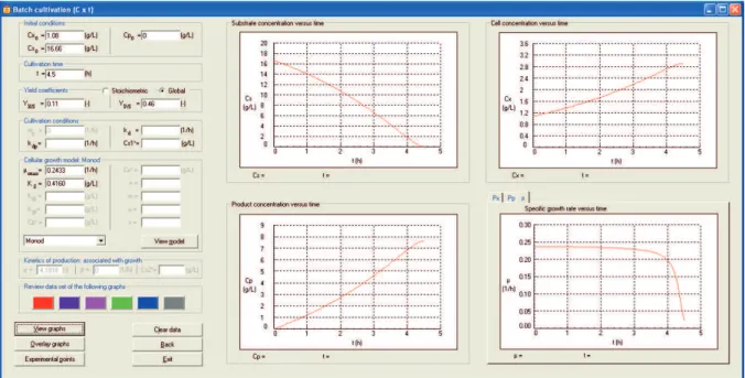
with recycle, and continuous in tanks connected in series without or with recycle), the type of analysis (graphical analysis for transient operations, or graphical analysis and operations at steady state), the kinetic model of cell growth, and the production type (associated, partially associated, or not associated with cell growth). After selection of the model and production kinetics, the cultivation conditions are inserted as shown in Fig. 9. In this window, the user can view the profiles of the substrate, cell, and product concentrations over time (“View graph”), and simulate the

The experimental data of substrate, cell, and product concentrations, as a function of time, can be added using the option “Experimental points” (Fig. 10), when selecting batch and fed batch cultivation modes. To illustrate this step, experimental data were added in Case Study 2. The user can choose which experimental points will be added, the exhibition mode, and the color and symbol used for the experimental datamarkers. After adding the experimental points, the cultivation conditions window is reopened (Fig. 11), displaying the graphs containing the experimental data and the simulation curves. The quality of the simulation can be seen from Fig. 11, since the experimental data of Badino and Hokka (1999) lie very close to the simulation values. In addition, the software allows the user to modify the kinetic parameters in order to improve the visual fitting of the kinetic model to the experimental data, enabling observation of the sensitivity of the model with respect to the kinetic parameters.

SimulaFerm has options available to copy and save the graph, remove or insert gridlines, and enlarge the graph. The simulation data can be saved in files with extensions “*.abr” or “*.dat”, using the menu “File/Save simulated data as”. This enables the data to be used in other programs (such as Microsoft Excel® _{or Origin}®_{). The input data} (cultivation conditions) can also be saved for future use.

The program includes a help file containing information about its resources and the theory of bioprocess kinetics and bioreactor analysis. The animation of cell growth models

is another option that can aid students and researchers, because it is possible to choose one of the available cell growth models and vary its parameter values, at the same time observing the results of the changes in the graph of μ versus C_S. The user can compare the results of the chosen model with those of the classical Monod model.

The AnaBioPlusprogram is available for download at the following website: http://www.deq.ufscar.br/ downloads/anabioplus.zip

CONCLUSIONS

The AnaBioPlus software package has great potential for teaching and research purposes involving the analysis of bioreactors. It is a non-commercial software package consisting of two programs: OptimusFerm and SimulaFerm. OptimusFerm is software for estimating the kinetic parameters of cell growth kinetic models, while SimulaFerm is a simulator for bioprocesses in different types of bioreactor configuration. The use of OptimusFerm and SimulaFerm was illustrated here by considering two example problems involving the estimation of kinetic parameters and simulation of a bioprocess. Good results were obtained for the estimated parameters and the simulation of the batch mode bioprocess, indicating that AnaBioPlus is a very useful tool for both purposes. Furthermore, the package has a user-friendly interface, which allows the user easy access to program resources.

NOMENCLATURE

B: concentration factor - ratio between cell concentrations in recycle and bioreactor outlet stream (-)

b_i: estimated parameters (-)

b_iinf_{: lower bounds of the parameters (-)} b_isup_{: upper bounds of the parameters (-)}

c: fraction of outlet stream leaving the bioreactor without passing through the cell separation unit (-)

C_P: product concentration (g.L-1₎

C_P0: initial product concentration or inlet product concentration (g.L-1₎

C_P*_{: critical value of product concentration to product} inhibition (g.L-1₎

C_P1: product concentration at bioreactor outlet stream in continuous cultivation with external recycle (g.L-1₎

C_Pn: product concentration in tank n (g.L-1₎ C_Pn-1: product concentration in tank n-1 (g.L-1₎ C_S: substrate concentration (g.L-1₎

C_S0: initial substrate concentration or inlet substrate concentration (g.L-1₎

C_S1*_{: critical substrate concentration at which cell} death begins (g.L-1₎

C_S2*_{: critical substrate concentration at which product} formation begins (g.L-1₎

C_Sf: substrate concentration in the feed (g.L-1₎ C_Sn: substrate concentration in tank n (g.L-1₎ C_Sn-1: substrate concentration in tank n-1 (g.L-1₎ C_X*_{: critical value of cell concentration to cell}

inhibition (g.L-1₎ C_X: cell concentration (g.L-1₎

C_X0: initial cell concentration or inlet cell concentration (g.L-1₎

C_Xn: cell concentration in tank n (g.L-1₎ C_Xn-1: cell concentration in tank n-1 (g.L-1₎ DE: differential evolution

EAs: evolutionary algorithms

F: culture medium feed volumetric flow rate (L.h-1₎ h: decline factor of cellular concentration to pass

through the separation unit k_d: cell death constant (h-1₎

k_dp: product degradation constant (h-1₎ K_IP: product inhibition constant (g.L-1₎ K_IS: substrate inhibition constant (g.L-1₎ K_S: saturation constant (g.L-1₎

K_SX: constant of Contoismodel(g.g-1₎ m: parameter of Lee model (-)

m_s: maintenance energy coefficient (h-1₎ n: parameter of Levenspiel model (-) NE: number of experimental data NP: number of estimated parameters

R: recycle ratio - ratio between the volumetric flow rates of recycle and outlet process streams (-) r_DP: rate of product degradation (g.L-1_.h-1₎

r_DPn: rate of product degradation in tank n (g.L-1_.h-1₎ r_D: rate of cell death (g.L-1_.h-1₎

r_Dn: rate of cell death in tank n (g.L-1_.h-1₎ r_P: rate of product formation (g.L-1_.h-1₎

r_Pn: rate of product formation in tank n (g.L-1_.h-1₎ r_S: rate of substrate consumption (g.L-1_.h-1₎

r_Sm: rate of consumption of substrate for maintenance energy (g.L-1_.h-1₎

r_SP: rate of consumption of substrate for product formation (g.L-1_.h-1₎

r_SX: rate of substrate consumption for biomass production or for cell growth (g.L-1_.h-1₎ r_X: rate of cell growth (g.L-1_.h-1₎

r_Xn: rate of cell growth in tank n (g.L-1_.h-1₎ T: temperature (°C)

t: time of bioprocess (h) u: parameter of Moser model (-) V: reactor volume (L)

x_Pci: dimensionless calculated product concentration (-)

x_Pei: dimensionless experimental product concentration (-)

x_Sci: dimensionless calculated substrate concentration (-)

x_Sei: dimensionlessexperimental substrate concentration (-)

x_Xci: dimensionless calculated cell concentration (-) x_Xei: dimensionless experimental cell concentration (-) Y_X/S: global cell yield coefficient (g.g-1₎

Y_G: true cell yield coefficient (g.g-1₎ Y_P/S: global product yield coefficient (g.g-1₎ Y_P: true product yield coefficient (g.g-1₎

Greek letters

α: constant for growth-associated product formation (-)

β: constant for non-growth-associated product formation (g.g-1_.h-1₎

µ: specific growth rate (h-1₎

µ_max: maximum specific growth rate (h-1₎ m_n: specific growth rate in tank n (h-1₎ v: parameter of Wu model (-)

Φ: objective function to be minimized in parameters estimation

ACKNOWLEDGMENTS

FAPESP (São Paulo State Research Funding Agency, Brazil), CNPq (National Council for Scientific and Technological Development, Brazil,grant #431460/2016-7), and CAPES (Coordination for the Improvement of Higher Educational Personnel, Brazil).

REFERENCES

Aiba S., Shoda M., Nagatani M., Kinetics of product inhibition in alcohol fermentation, Biotechnology and Bioengineering, 10, p.845-864 (1968).

Aleman-Meza B., Yu Y., Schüttler H.B., Arnold J., Taha T.R., KINSOLVER: A simulator for computing large ensembles of biochemical and gene regulatory networks, Computers & Mathematics with Applications, 57, p.420-435 (2009). Andrews J.F., A mathematical model for the continuous culture of

microorganisms utilizing inhibitory substrates, Biotechnology and Bioengineering, 10, p.707-723 (1968).

Badino A.C., Hokka C.O., Laboratory experiment in biochemical engineering: ethanol fermentation, Chemical Engineering Education, 33, p.54-70 (1999).

Baptista-Neto A., Gouveia E.R.; Badino A.C.; Hokka, C.O., Phenomenological model of the clavulanic acid production process utilizing Streptomyces clavuligerus, Brazilian Journal of Chemical Engineering, 17, p.809-818 (2000).

Bard, Y. Nonlinear Parameter Estimation. Academic Press, New York (1974).

Barshop B.A., Wrenn R.F., Frieden C., Analysis of numerical methods for computer simulation of kinetic processes:

Development of KINSIM - a flexible, portable system,

Analytical Biochemistry, 130, p.134-145 (1983).

Contois D.E., Kinetics of bacterial growth: relationship between

population density and specific growth rate of continuous

cultures, Journal of General Microbiology, 21, p.40-50 (1959).

Garvey T.D., Lincoln P., Pedersen C.J.P., Martin D., Johnson M., BioSPICE: Access to the most current computational tools for biologists, Journal of Integrative Biology, 7, p.411-420 (2003).

Ghosh A., Das S., Chowdhury A., Giri R., An improved

differential evolution algorithm with fitness-based adaptation

of the control parameters, Information Sciences, 181, p.3749-3765 (2011).

Himmelblau, D.M. Process Analysis by Statistical Methods.John Wiley & Sons, Inc., New York (1970).

Hoops S., Sahle S., Gauges R., Lee C., Pahle J., Simus N., Singhal M., Xu L., Mendes P., Kummer U., COPASI - a Complex PAthway Simulator, Bioinformatics, 22, p.3067-3074 (2006). Hoppe G.K., Hansford G.S., Ethanol inhibition of continuous

anaerobic yeast growth, Biotechnology Letters, 4, p.39-44 (1982).

Johnson K.A., Simpson Z.B., Blom T., Global Kinetic Explorer:

A new computer program for dynamic simulation and fitting

of kinetic data, Analytical Biochemistry, 387, p.20-29 (2009). Kierzek A.M., STOCKS: STOChastic Kinetic Simulations of

biochemical systems with gillespie algorithm, Bioinformatics, 18, p.470-481 (2002).

Lee J.M., Polland J.F., Coulman G.A., Ethanol fermentation with cell recycling: computer simulation, Biotechnology and Bioengineering, 25, p.497-511 (1983).

Levenspiel O., The Monod equation: a revisit and a generalization to product inhibition situations, Biotechnology and Bioengineering, 22, p.1671-1687 (1980).

Loew L.M., Schaff J.C., The Virtual Cell: a software environment

for computational cell biology, Trends Biotechnology, 19, p.401-406 (2001).

Long W., Liang X., Huang Y., Chen Y., A hybrid differential

evolution augmented Lagrangian method for constrained numerical and engineering optimization, Computer-Aided Desig, 45, p.1562-1574 (2013).

Mendes P., GEPASI: A software package for modeling the dynamics, steady states and control of biochemical and other systems, Computer Applications in the Biosciences, 9, p.563-571 (1993).

Monod J., Recherchessur la croissance des cultures bactériennes, Hermann & Cie., Paris (1942).

Moser H., The dynamics of bacterial population maintained in the chemostat. Carnegie Institute of Washington, Washington (1958).

Murphy T.A., Young J.D., ETA: Robust software for

determination of cell specific rates from extracellular time

courses, Biotechnology and Bioengineering, 110, p.1748-1758 (2013).

Nelles, O. Nonlinear System Identification: From Classical

Approaches to Neural Networks and Fuzzy Models. Berlin, Heidelberg: Springer-Verlag (2001).

Novère N.L., Shimizu T.S., STOCHSIM: modelling of stochastic biomolecular processes, Bioinformatics, 17, p.575-576 (2001).

Pan Q., Suganthan P.N., Wang L., Gao L., Mallipeddi R., A

differential evolution algorithm with self-adapting strategy

and control parameters, Computers & Operations Research, 38, p.394-408 (2011).

Phan-Thien Y.N., BioMASS v2.0: A new tool for bioprocess simulation. Master’s thesis in Science Biosystems Engineering, Clemson University, United States (2011). Rocha M., Rocha I., Rocha O., Maia P., OptFerm PT Universityof

Minho, Minho. http://darwin.di.uminho.pt/optferm/index. php/Main_Page. Accessed 02 Oct 2015 (2009).

Silva F.H., Jesus C.D.F., Cruz A.J.G., Badino A.C., Anabio 2.0: um programa para estimativa de parâmetros cinéticos e análise de biorreatores. In: XV Simpósio Nacional de Bioprocessos, Recife (2005).

Silva F.H., Moura L.F., Badino A.C., AnaBio 1.0: Um Programa para Análise de Biorreatores. In: XIV Simpósio Nacional de Fermentações, Florianópolis (2003).

Stiles J.R., Bartol T.M., In: Schutter E (ed) ComputationalNeuroscience: RealisticModelling for Experimentalists. CRC Press, Boca Raton (2001).

Soares R.P.,Secchi, A.R., EMSO: A new environment for modelling, simulation and optimization. Computer Aided Chemical Engineering, 1, p. 947–952 (2003).

Storn R., Price K., Differential Evolution - A simple and efficient

spaces, Journal of Global Optimization, 11, p.341-359 (1997). Svir I.B., Klymenko O.V., Platz M.S., ‘KINFITSIM’- a software

to fi t kinetic data to a user selected mechanism, Computer

&Chemistry, 26, p.379-386 (2002).

Tomita M., Hashmoto K., Takahasi K., Shimizu T.S., Matsuzaki Y., Miyoshi F., Saito K., Tanida S., Yugi K., Venter J.C., Hutchison C.A., E-CELL: Software environment for

whole-cell simulation, Bioinformatics, 15, p.72-84 (1999).

Wu Y.C., Hao O.J., Ou K.C., Scholze R.J., Treatment of leachate

from solid waste landfi ll site using a two-stage anaerobic fi lter, Biotechnology Bioengineering, 31, p.257-266 (1988).

Zimmerle C.T., Frieden C., Analysis of progress curves by simulations generated by numerical integration, Biochemical Journal, 258, p.381-387 (1989).

dx.doi.org/10.1590/ 0104-6632.20170344s20150673erratum

ERRATUM

Erratum of article

Oliveira, C. M., Jesus, C. D. F., Ceneviva, L. V. S., Silva, F. H., Cruz, A. J. G., Costa, C. B. B., & Badino, A. C.. (2017). AnaBioPlus: a new package for parameter estimation and simulation of bioprocesses. Brazilian Journal of Chemical Engineering, 34(4), 1065-1082. https://dx.doi.org/10.1590/0104-6632.20170344s20150673

In the page 1067, where it reads

“in order to avoid excessiveweightings in the data set.”, it should read

“in order to avoid excessive weightings in the data set.”

In the page 1069, where it reads

“Good descriptions of the theory of parameter estimation for non-linear model scan be found inHimmelblau (1970), Bard (1974), and Nelles (2001).”,

it should read

“Good descriptions of the theory of parameter estimation for non-linear model can be found in Himmelblau (1970), Bard (1974), and Nelles (2001).”

In the page 1074, where it reads

“In this example, m_max and KS were the estimated parameters of the Monod model (Eq. 3, Table 1).”, it should read

“In this example, μ_max and KS were the estimated parameters of the Monod model (Eq. 3, Table 1).”

In the page 1074, where it reads

“The estimated parameter values and confi dence intervals were m_max=0.2056±0.0006 h-1 _{and K}

S=3.49±0.29 g.L -1_.”,

it should read

“The estimated parameter values and confi dence intervals were μ_max=0.2056±0.0006 h-1 _{and K}

S=3.49±0.29 g.L -1_.”

In the page 1076, where it reads

“The help fi le is available from the “Help/Help topics”menu.”

it should read

“The help fi le is available from the “Help/Help topics” menu.”

In the page 1076, where it reads

“Estimation of the kinetic parameters (m_max and K_S) for this problem employed ...”,

it should read

“Estimation of the kinetic parameters (μ_max and K_S) for this problem employed ...”

In the page 1080, where it reads “m_n: specifi c growth rate in tank n (h-1_)”, it should read

“μ_n: specifi c growth rate in tank n (h-1_)” “in order to avoid excessiveweightings in the data set.”, it

“in order to avoid excessive weightings in the data set.”

for non-linear model scan be found inHimmelblau (1970), for non-linear model scan be found inHimmelblau (1970),

for non-linear model can be found in Himmelblau (1970), for non-linear model can be found in Himmelblau (1970),

“In this example, m_max and KS were the estimated

μmax and KS were the estimated

were m_max=0.2056±0.0006 h

μmax=0.2056±0.0006 h

topics”menu.”

topics” menu.”

“Estimation of the kinetic parameters (m_max and K

“Estimation of the kinetic parameters (μ “Estimation of the kinetic parameters (

“Estimation of the kinetic parameters ( _max and K

“m_n: specifi c growth rate in tank n (h

“μ