www.hydrol-earth-syst-sci.net/13/1921/2009/ © Author(s) 2009. This work is distributed under the Creative Commons Attribution 3.0 License.
Earth System
Sciences
Hydrological model performance and parameter estimation in
the wavelet-domain
B. Schaefli1and E. Zehe2
1Faculty of Civil Engineering and Geosciences, Water Resources Section, Delft University of Technology, The Netherlands 2Institute of Water and Environment, Dept. for Hydrology and River Basins Management, Technische Uni. M¨unchen,
Germany
Received: 5 March 2009 – Published in Hydrol. Earth Syst. Sci. Discuss.: 20 March 2009 Revised: 28 September 2009 – Accepted: 28 September 2009 – Published: 19 October 2009
Abstract. This paper proposes a method for rainfall-runoff model calibration and performance analysis in the wavelet-domain by fitting the estimated wavelet-power spectrum (a representation of the time-varying frequency content of a time series) of a simulated discharge series to the one of the corresponding observed time series. As discussed in this pa-per, calibrating hydrological models so as to reproduce the time-varying frequency content of the observed signal can lead to different results than parameter estimation in the time-domain. Therefore, wavelet-domain parameter estimation has the potential to give new insights into model performance and to reveal model structural deficiencies. We apply the pro-posed method to synthetic case studies and a real-world dis-charge modeling case study and discuss how model diagnosis can benefit from an analysis in the wavelet-domain. The re-sults show that for the real-world case study of precipitation – runoff modeling for a high alpine catchment, the calibrated discharge simulation captures the dynamics of the observed time series better than the results obtained through calibra-tion in the time-domain. In addicalibra-tion, the wavelet-domain performance assessment of this case study highlights the fre-quencies that are not well reproduced by the model, which gives specific indications about how to improve the model structure.
1 Introduction
Most hydrological models have parameters that cannot be related to some measurable catchment characteristics and have to be calibrated. Classically, this calibration determines the best parameter values such as the simulations match as closely as possible one or several observed system outputs
Correspondence to:B. Schaefli (b.schaefli@tudelft.nl)
(for an overview of calibration methods, see, e.g. Gupta et al., 2005). The uncertainties inherent in the simulations of such calibrated models (e.g. Beven and Freer, 2001; Vrugt et al., 2003; Kavetski et al., 2006a) and the question how to reduce them are subject to intense research. Current strate-gies include a better description and understanding of the uncertainty inherent in the involved natural processes (e.g. Zehe et al., 2005), in the observation of these processes (e.g. Nic´otina et al., 2008) or in the mathematical representation of these processes (e.g. Kavetski et al., 2006b). In parallel, the question how to increase the value of observed data through an improved extraction of its information content receives a constantly growing interest (e.g. Herbst and Casper, 2008; Reusser et al., 2008; Yilmaz et al., 2008).
As a good simulation should mimic the dynamics underly-ing an observed time series, it is temptunderly-ing to think that explic-itly assessing how well a model reproduces the autocorrela-tion properties of an observed system response is a promis-ing choice for model calibration. Keeppromis-ing, furthermore, in mind that time series of hydrological signatures exhibit peri-odicity at different time scales, model performance measures that are based on spectral information appear rather appeal-ing. A straight forward choice is of course the power-density spectrum of a process which equals the Fourier transform of its autocorrelation function (Priestley, 1981). This idea is in-deed not new; Whittle (1953) proposed a method for parame-ter estimation in the Fourier-domain matching the theoretical density spectrum of the model to the estimated power-density spectrum of the process observations. The Whittle estimator has recently been applied to rainfall-runoff models by Montanari and Toth (2007).
Whittle’s Fourier-domain estimator is a consistent approx-imation of the classical time-domain likelihood. For in-finitely long time series, it will, thus, yield the same result as time-domain estimation (see, e.g. Hannan, 1973; Yao and Brockwell, 2006). However, as shown by Contreras-Crist´an et al. (2006), it can produce unreliable estimates for non-Gaussian processes or show an important loss of efficiency if the autocorrelation of the process is high.
1.1 Objectives of this paper
The overall idea is to present a new performance measure to assess how closely the time-varying frequency content of a simulated time series matches the time-varying frequency content of the observed series. This objective function is based on a continuous wavelet transform that yields a rep-resentation of the time-varying frequency content of an ob-served time series – as opposed to a Fourier transform, where the moment of occurrence of the different frequencies is not preserved. The wavelet transform is particularly useful for application to natural processes, such as discharge, that in-tegrate various time-varying small scale processes at a larger spatial scale and that, thus, have time-varying autocorrelation properties. This time-variation of the hydrological response of an ecosystem is, of course, partly induced by the time-variation of the relevant input processes, e.g. precipitation and temperature. Furthermore, the rainfall-runoff response is essentially nonlinear, including threshold behavior (Zehe et al., 2007; Bl¨oschl and Zehe, 2005). The input frequencies are thus nonlinearly filtered by the catchment and its biotic (e.g. vegetation) and abiotic characteristics. In glaciated catch-ments, the real-world case study of this paper, the overall time-variability is particularly pronounced since discharge is induced by a combination of rainfall, ice and snowmelt (see Fig. 1a).
We will give evidence that an objective function that mea-sures explicitly how well the time-varying frequency content of an observed series is reproduced can provide important
40
08/02 30/03 19/08 08/07 27/08 16/10 05/12 0
20
Rhone obs 1995 Rhone sim 1995
08/01 27/02 18/04 07/06 27/07 15/09 04/11 24/12 0
20 40
Date
Discharge (mm/day)
Rhone obs 1997 Rhone sim 1997 a)
b)
Discharge (mm/day)
Time step (days)
400 500 600 700 800 900 1000
0 10 20
0 10 20
Exp. 2 Exp. 3
Exp. 2, perturbed series
400 500 600 700 800 900 1000
Fig. 1. (a) Observed discharge time series of the Rhone River at Gletsch and corresponding (time-domain) calibrated time series (Nash valueLN=1-RN=0.94), for the years 1995 (top) and 1997
(bottom);(b)synthetic discharge time series generated with GSM-SOCONT, unperturbed series for experiments 2 and 3 (top), per-turbed series for experiment 2 (bottom).
and new pieces of information to the puzzle of understanding performance and structural deficits of hydrological models. Such an objective function allows, furthermore, estimation of model parameters. We intend to show that such an ap-proach represents a very valuable opportunity compared to parameter estimation in the time domain. As the suggested approach depends crucially on how similarity between es-timated wavelet-power spectra is defined, this will be dis-cussed in detail in Sect. 3 after an introduction to contin-uous wavelet transform in Sect. 2. We then illustrate the advantages and drawbacks of parameter estimation in the wavelet-domain through simple examples and synthetic case studies, i.e. using synthetic data generated either with a sim-ple statistical model or with a conceptual, reservoir-based rainfall-runoff transformation model (Sects. 4 and 5). Fi-nally, we apply the wavelet-domain objective function to pa-rameter estimation of the GSM-SOCONT (Schaefli et al., 2005) model for a highly glacierized catchment in the Swiss Alps. Based on this case study, we discuss the potential of wavelet-domain calibration and performance analysis and show how it can contribute to improve the structure of hy-drological models (Sect. 5). The main conclusions and open questions are summarized in Sect. 6.
2 Continuous wavelet spectral analysis
of occurrence. Wavelet analysis, in turn, results in a time-frequency (or time-scale) representation of the signal. In-stead of decomposing a signal into constituent harmonic functions as in Fourier analysis, wavelet analysis transforms a signal into scaled and translated versions of an original (mother) wavelet. Compared to a simple windowed Fourier transform, as suggested by Gabor (1946), wavelet transform has the main advantage of adjusting intrinsically the resolu-tion to the analyzed scale (e.g. Daubechies, 1992).
In hydrology, continuous wavelet transform became popu-lar in different types of applications; it is for example used to characterize river regimes and to detect how discharge is re-lated to climate variability indices (e.g. Labat, 2005) or to qualitatively analyze how certain features of the meteoro-logical input time series are transferred to the hydrometeoro-logical system output (e.g. Gaucherel, 2002; Lafreni`ere and Sharp, 2003; Schaefli et al., 2008). Lane (2006) was the first to use it to investigate rainfall-runoff models, namely to investigate the impact of perturbing single model parameters on the re-sulting hydrographs.
Even though wavelet spectral analysis has found a wide spread application, few papers present all the mathematical details which we judge to be necessary to understand this paper and to interpret the results. Therefore, the following section might seem rather detailed to the reader with a back-ground in wavelet spectral analysis.
2.1 Continuous wavelet transform
Given a stochastic process X(t ), its wavelet transform
Wg[τ, s|X(t )] at timeτ and scaleswith respect to the
cho-sen waveletg(t )is
Wg[τ, s|X(t )]=
Z 1
c(s)g
∗t−τ
s
X(t )dt (1)
whereg∗ denotes the complex conjugate of g andc(s) is a normalization constant (see Sect. 2.3). For a detailed discussion of continuous wavelet transform (CWT) and for example the requirements on the wavelet g(t ), we refer the reader to the comprehensive literature (e.g. Daubechies, 1992; Holschneider, 1998).
The choice of the waveletg(t )depends on the type of ap-plication. In geosciences applications, the Morlet wavelet is frequently used (for a short discussion of how to choose a wavelet for hydrological applications, see Schaefli et al., 2008):
gm(θ )=exp(iω0θ )exp − θ2
2 !
(2)
wherei=√−1 andθ=(t−τ )/s. The parameterω0 adjusts
the time/scale resolution. In the present application, we use
ω0=6, a choice that has empirically been shown to work well
for geosciences applications (Labat, 2005; Si and Zeleke, 2005; Torrence and Compo, 1998).
For a Morlet wavelet, the relationship between the scales
and the frequencyf reads as (e.g. Holschneider, 1998): 1
f =
4π s ω0+
q 2+ω02
(3)
Therefore, forω0=6,f≈1/s.
It is important to note that the CWT transforms a time series from one to two dimensions (time and scale). This transformation re-uses the same original information several times and results, therefore, in a considerable amount of re-dundancies. The inherent correlations of a CWT, given by the reproducing kernel (e.g. Holschneider, 1998), make sta-tistical analysis of wavelet-power spectra a non-trivial task (Maraun et al., 2007; Schaefli et al., 2008). They represent a fundamental difference to estimated Fourier power-density spectra where neighboring frequencies are asymptotically in-dependant.
2.2 Wavelet-power spectrum
Analogue to Fourier analysis, the wavelet-power spectrum (WPS) is defined as the wavelet transform of the autocovari-ance function, which for a nonstationary processX(t )can be written as (e.g. Shumway and Stoffer, 2006):
acv [ℓ, η|X(t )]≡ E
(X(η)−E [X(η)])conj(X(η+ℓ)−E [X(η+ℓ)]) (4) whereηis the time argument of the autocovariance function andℓis the lag from timeη. E [·] is the expected value and “conj” denotes here the complex conjugate (elsewhere de-noted by *). For simplicity of notation, let’s assume in the following thatX(t )is a zero-mean process, i.e. E [X(t )]=0 for allt. The WPS does becomes (e.g. Holschneider, 1998):
Sg[τ, s|X(t )]≡Wgτ, s
E
X(η)conj(X(η+ℓ))
=EhWg[τ, s|X(η)]Wg∗[τ, s|X(η+ℓ)]
i (5) This last equation is often written in the following short form:
Sg[τ, s|X(t )]≡E
h
Wg[τ, s|X(t )]
2i
(6) The exact WPS of observed or simulated processes is gen-erally unknown; we can estimate it based on the CWT of observed process realizations (observed time series):
ˆ Sg
h
τ, s|x(m)(t ),µ(t )ˆ i=
Wg[τ, s|x
(m)(t ) − ˆµ(t )]
2 (7)
where Sˆgτ, s|x(m)(t ),µ(t )ˆ is an estimator of Sg[τ, s|X(t )]. h·i denotes the averaging operator, x(m)(t )
obtained based on a single realizationx(t )=x(1)(t )of length
N:
ˆ
Sg[τ, s|x(t )]=
Wg
τ, s|x(t )− ˆµ
2
(8) where the estimatorµˆ is obtained as the average of the real-ization, i.e.µˆ=N1
N
P
k=1 x(k).
In analogy to Fourier analysis, this estimatorSˆg[τ, s|x(t )]
is called the wavelet periodogram. It is computed at a finite number of scales between the lowest and the highest resolv-able scales that depend on the sampling time step and the number of sampled time steps. The selected scales are usu-ally:
si =s02
i−1
Nvoice (9)
withi=1,..,Nvoice×Noctave+1. The lowest calculated scale
iss0corresponding to a frequency lower than or equal to the
Nyquist frequency (i.e. half the sampling frequency, see, e.g., Priestley, 1981) and the highest scale iss0×2Noctave where Noctave denotes the number of octaves (i.e. powers of two),
andNvoice the number of voices (i.e. calculated scales) per
octave.
It is important to note that wavelet analysis has the sub-tlety that, since neighboring points in time and scale are cor-related, the wavelet periodogram looks smooth even if the fluctuations around the true wavelet-power spectrum are not smaller than for a (Fourier) periodogram (see Maraun and Kurths, 2004). Accordingly, as for the Fourier periodogram, the wavelet periodogram has to be smoothed to obtain a con-sistent estimator of the true wavelet-power spectrum (see, e.g. Maraun and Kurths, 2004). For the present application that uses the difference between the wavelet periodograms of two time series for model calibration, the consistency of the estimator is, however, of no relevance.
2.3 Normalization of the wavelet transform
The choice of the normalization constant in Eq. (1) is not un-ambiguous. It can in principle be chosen arbitrarily (Kaiser, 1994, p. 62) and just as in Fourier analysis, different conven-tions are in use.
To compute the wavelet-power-based performance crite-ria, we use theL2-norm preserving normalizationc(s)=√s, which ensures that (Kaiser, 1994, p. 63)
1
c(s)g
t
−τ s
2 =
∞ Z
−∞
1
√ sg
u
−τ s
2 du
=
∞ Z
−∞
|g (v)|2dv= kg (t )k2=cst (10)
3 Wavelet periodogram – based performance assessment
3.1 Visual inspection
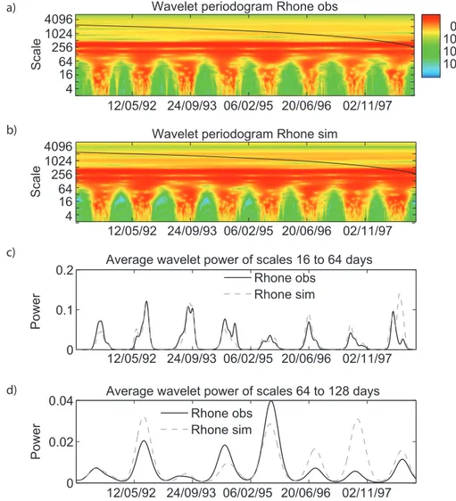
Wavelet periodograms (i.e. estimated wavelet-power spectra) have the potential to efficiently distinguish between time se-ries that seem to be similar in the time-domain but that have a (locally) different frequency content and, thus, locally dif-ferent autocorrelation properties. We illustrate this poten-tial based on the wavelet periodograms of the simulated and of the observed daily discharge series from the Rhone River at Gletsch. Further details on these time series are given in Sect. 4. The simulated series appears to be very similar to the observed series (Fig. 1a), with a linear correlation of 0.97 or, using the classical hydrological performance criterion pro-posed by Nash and Sutcliffe (1970), a Nash value of 0.94 (see Sect. 4).
The visual interpretation of the 2-D wavelet periodograms (Fig. 2a and b) is difficult and error prone (Maraun and Kurths, 2004; Maraun et al., 2007). Therefore, Fig. 2c and d show the so-called wavelet bands that correspond to the scale-average wavelet-power over given ranges of scales, where the average power is defined as the scale-weighted sum of the wavelet-power (Torrence and Compo, 1998). The bands are normalized by the variance of the time series. As Fig. 2c and d in conjunction with Fig. 1a illustrate, such a plot reveals differences that are not readily seen in the original data. We see namely that for the band of scales 64 days to 128 days, the calibrated model does not correctly re-produce the dynamics. These differences would also be vis-ible in a detailed inspection of the time series, by comparing the weekly, monthly and seasonal statistics or by subtracting the series from each other and analyzing the obtained “resid-uals”. However, inspecting wavelet bands provides several views of the signal at the same time and has the main advan-tage of yielding a rapid overview over the differences. 3.2 Wavelet performance measure
We propose a method for the estimation of model parame-ters in the wavelet-domain. It is based on the following hy-potheses: (i) the dynamics of two processes are similar if their time-varying autocorrelation properties are similar; (ii) these autocorrelation properties can be estimated based on the wavelet periodograms of process realizations. For model calibration, this translates into the assumption that the more similar the wavelet periodograms of a simulated and an ob-served time series are, the better the model mimics the be-havior of the natural system.
0 0.1
0.2 Average wavelet power of scales 16 to 64 days
Power
0 0.02
0.04 Average wavelet power of scales 64 to 128 days
Power
Rhone obs Rhone sim
Rhone obs Rhone sim
12/05/92 24/09/93 06/02/95 20/06/96 02/11/97
12/05/92 24/09/93 06/02/95 20/06/96 02/11/97
t
10 10 10
0-2
-4 -6 a)
b)
c)
d)
12/05/92 24/09/93 06/02/95 20/06/96 02/11/97
12/05/92 24/09/93 06/02/95 20/06/96 02/11/97 Wavelet periodogram Rhone obs
Scale
4 16 64 256 1024 4096
Scale
4 16 64 256 1024 4096
Wavelet periodogram Rhone sim
Fig. 2.Estimated wavelet-power for the Rhone case study:(a)wavelet periodogram of the observed discharge (zoom on the 2nd half of the available time series, black line: cone of influence),(b)wavelet periodogram of the simulated discharge,(c)average estimated wavelet-power of both series between the scales of 16 days and 64 days,(d)same as (c) but between the scales of 64 days and 128 days.
choice of this distance metric has to take into account the fact that in the wavelet periodogram neighboring scales and neighboring time steps are correlated.
We use a metric similar to the Kolmogorov-Smirnov dis-tance, which is classically used to measure the distance of the probability distributions of two samples and which equals the maximum distance between the cumulative distribution func-tions. This metric is particularly useful to measure whether at a given time stept, the power of the observed and of the simulated wavelet periodogram is similarly distributed over all scales: it is sensitive to the shape of the power distribu-tion over the scales but compared to a squared error-based metric, it is much less sensitive to slight shifts in peaks and to the chosen normalization constant in Eq. (1).
The cumulative wavelet-periodogram Cˆg[τ, s|x(t )] is
computed as:
ˆ
Cg[τ, s|x(t )]= s
X
k=s0
ˆ
Sg[τ, k|x(t )] (11)
wheres=s0, . . . ,smax(τ). smaxis the maximum scale
The Kolmogorov-Smirnov distance Dg[τ|x(t ), y(t )] at
time stepτ between two process realizationsx(t )andy(t )
becomes:
Dg[τ|x(t ), y(t )]=max
ˆ
Cg[τ, s|x(t )] ˆ
Cg[τ, s=smax|x(t )]
− Cˆg[τ, s|y(t )] ˆ
Cg[τ, s=smax|y(t )]
(12)
where Cˆg[τ,s|x(t )] ˆ
Cg[τ,s=smax|x(t )]=
s
P
k=s0 ˆ
Sg[τ,k|x(t )]
smax
P
k=s0 ˆ
Sg[τ,k|x(t )]
is the normalized cu-mulative wavelet periodogram of the process realizationx(t )
at time stepτ.
A good simulation should have a wavelet periodogram that fits the periodogram of the observed series at all time steps. Accordingly, the overall wavelet periodogram efficiency cri-terion, RW, averages Dg[τ|x(t ), y(t )] over all time steps.
For an observed time seriesy(t )and the corresponding sim-ulated seriesx(t|ϕ)this becomes
RW[ϕ|x(t|ϕ), y(t )]=
1
N N
X
τ=1
Dg[τ|x(t|ϕ), y(t )] (13)
whereN is the total number of time steps and ϕ a vector
containing all model parameters.RWtakes values between 0
and 1 and has to be minimized during calibration.
In order to be applicable to parameter estimation, a dis-tance metric has to fulfill formal requirements (e.g. Weis-stein, 2008). For some general distance metricD(A,B) be-tweenAandBit has to hold that (i)D(A, B)≥0, ∀A, B, ii)
D(A, B)=D(B, A)(iii)D(A, B)=0 if and only ifA=Band (iv) D(A, C)≤D(A, B)+D(B, C). For the wavelet-based distance measureDg[τ|x(t ), y(t )], it follows directly from
its definition that conditions (i) and (ii) hold. Condition (iv), the so-called triangle inequality, holds since the maxi-mum distance between two monotonically increasing func-tions between 0 and 1 can never be bigger than the sum of the maximum distances between these two functions and a third function. SinceRW[·] results from a simple average of Dg[τ|x(t ), y(t )] over allτ, conditions (i), (ii) and (iv) also
hold for RW[·]. Condition (iii) does not necessarily hold
forDg[τ|x(t ), y(t )]: two process realizationsx(t )andy(t )
could, in theory, have locally exactly the same distribution of wavelet-power without havingx(t )=y(t ),∀t. However, it holds thatRW[·]=0 if and only ifDg[τ|x(t ), y(t )]=0 ∀τ
which impliesx(t )=y(t ). We conclude thatRW[·] satisfies
the formal conditions of a distance metric.
RW measures whether the wavelet-power content at every
time-step is distributed similarly in a simulated series and a reference series, i.e. it measures differences in the autocorre-lation properties at a given time step. Accordingly, it does not explicitly measure differences in the mean or in the variance of two time series.
As in every parameter estimation procedure, preserving the mean, or in physical terms the mass balance, is a very important criterion to accept or reject simulations and the underlying model. Traditional time-domain calibration en-sures preservation of the mean either through the assump-tions on the residual distribution (e.g. zero-mean Gaussian residuals, Kavetski et al., 2006b) or through explicit exclu-sion of parameter sets leading to a too high bias between the observation and the simulation (see, e.g., Montanari and Toth, 2007). We retain this last solution by deteriorating the wavelet performance criterionRW of a given simulation if
its bias exceeds a certain tolerance factor. The exact value of this tolerance factor has to be fixed empirically. For perfect model situations where the true (and hence unbiased) simula-tion exists, the tolerance factor does not affect the best iden-tified parameter set but restrains the search space. For real-world applications, this restriction of the search space might influence the best identified parameter set since it excludes not mass conservative, i.e. physically meaningless parameter sets.
In the present study, we use a tolerance factor of 10% for all case studies. For the real-world application, this choice is in line with the semi-automatic calibration method suggested by Schaefli et al. (2005). In general, the value of the toler-ance factor should reflect the available information about the observational uncertainties of the different terms of the wa-ter balance. The exact penalization procedure based on this tolerance factor is discussed in Sect. 4.3.3.
For general stochastic processes with stationary mean, variance and autocorrelation properties, these are a priori un-related properties and a good process model should preserve them. Discharge processes, on which we focus in the present paper, have a time-variable mean, variance and autocorrela-tion (see an example in Fig. 1). Since discharge results from a time-variable combination of different hydrological pro-cesses (infiltration, snowmelt etc.), these statistical proper-ties are strongly related. For such processes, as our empirical results show, preserving the mean and the time-varying auto-correlation properties ensures the preservation of the process variance.
We would like to add here that in the statistics literature, wavelet-based estimators have been proposed in the 1990s to estimate long-memory parameters (see Velasco, 1999, p. 107) but their statistical properties are analyzed only re-cently (e.g. Moulines et al., 2008). As the corresponding es-timation problems are very different from the scope of the present paper, we do not discuss them here.
4 Case studies
4.1 Synthetic case studies
model calibration experiments where the reference discharge series are generated with known parameter values. Three dif-ferent sets of synthetic discharge series are used. For exper-iment 1, we use the realization of an ARMAX process. For experiments 2 and 3, we use a realization of the hydrological model GSM-SOCONT, which is also used in the real-world case study.
Experiment 2 uses the classical model structure, whereas experiment 3 is based on a slightly modified model version including a time-varying parameter. Details about all syn-thetic experiments are given hereafter. Additional illustrative toy examples as well as a synthetic case study with the well-known HYMOD model (e.g. Schaefli and Gupta, 2007) can be found in (Schaefli and Zehe, 2009).
4.1.1 Input time series
The synthetic experiments have been designed to illustrate the differences between parameter estimation in the time-domain and in the wavelet spectral time-domain. We therefore use as external forcing a nonstationary precipitation series which is obtained by joining two precipitation series that have different statistical properties. To have a realistic sit-uation, these two individual series are surrogate series gen-erated based on the precipitation series observed at the sta-tion Bourg St. Pierre between 1903 and 1999, located in the Southern Swiss Alps (1620 m a.s.l., 7.21◦E, 45.95◦N), which is also used also for the real-world case study. The pre-cipitation in this area is known to have undergone a substan-tial modification over the last century (Frei and Sch¨ar, 2001; Schmidli and Frei, 2005). The generation of the nonstation-ary rainfall series involves the following steps: (i) Gener-ate a 250 days surrogGener-ate series based on the first 20 years of observed precipitation. The surrogate series is generated us-ing the so-called Iterative Amplitude Adjusted Fourier Trans-form (IAAFT) algorithm (Schreiber and Schmitz, 2000). This is a classical method to obtain surrogates by first taking the Fourier transform of a time series, replacing the phases by randomly drawn phases and then completing the inverse Fourier transform. (ii) Generate a 250 days surrogate series based on the last 20 years of observed precipitation. (iii) Contract both series.
For experiments 2 and 3, we generate a longer series, 10 years, and use the first half for calibration and the second half for validation.
4.1.2 Output time series
For experiment 1, the used ARMAX process is:
y(t )=a·y(t−1)+b1z(t−nk)+b2z(t−1−nk)+b3z(t−2−nk)(14) wheret is the time step, z(t ) is the input variable (in our case precipitation),nk is the delay parameter that is set to
4 andϕ=[a, b1, b2, b3] are the parameters to be inferred.
The reference exact series is generated using the following parameters: ϕ=[a,b1,b2,b3]=[−0.85,0.080, 0.018, 0.029].
The resulting series is perturbed with uncorrelated Gaussian noise having zero mean and standard deviation 0.4, corre-sponding to 25% of the standard deviation of the generated
y(t ).
Experiments 2 and 3 are based on a reference discharge se-ries simulated with the hydrological model GSM-SOCONT (Schaefli et al., 2005) (see also Sect. 4.) using the same pre-cipitation series as in experiment 1. We assume that there is no glacier cover and use a temperature time series cor-responding to a low land station (the station called Grono, 380 m a.s.l., 9.15◦E, 46.25◦N). This makes the discharge time series explicitly distinct from the real-world case study (see Sect. 4.2); in particular there is a less strong annual cycle of the discharge (see Fig. 1b).
For experiment 3, we generate a reference series with GSM-SOCONT having a time-variable snowmelt parameter (see Table 4) and then calibrate the model with a constant snowmelt parameter on this reference series. This experi-ment illustrates a typical example of model misspecification. For both experiments 2 and 3, the synthetic realizations are perturbed by adding white noise before the parameter cali-bration process (see results section for details).
4.2 Real-world case study
4.3 Parameter estimation
4.3.1 Reference performance criteria
For comparison purposes, we use the classical squared error-based Nash-Sutcliffe efficiency measure (Nash and Sutcliffe, 1970), called hereafter Nash value:
LN[ϕ|x(t|ϕ), y(t )]=1− N
P
t=1[
x(t|ϕ)−y(t )]2
N
P
t=1[
y(t )−E [y(t )]]2
(15)
wherey(t )is the observed discharge at time stept,x(t|ϕ)
is the simulated discharge given parameter setϕandN the
number of observed and simulated time steps.
We define a Nash-based performance measure to be mini-mized as follows
RN[ϕ|x(t|ϕ), y(t )]=1−LN[ϕ|x(t|ϕ), y(t )] (16)
For the synthetic case studies, where the (exact) best model parameter set exists, we also use a Fourier-domain perfor-mance measure based on the Whittle likelihood, computed according to Montanari and Toth (2007) as:
LFϕ|Jx(λ|ϕ), Jy(λ)=exp
"
−
N/2
X
j=1
log
Jx(λj|ϕ)+fe(λj|ϕ)+ Jy(λj) Jx(λj|ϕ)+fe(λj|ϕ)
#
(17) whereλj=2πj/N are the Fourier frequencies. Jxis the
pe-riodogram of the simulated discharge time series andJythe
periodogram of the observed discharge time series.feis the
Fourier-power spectrum of the modeling error (for details, re-fer to Montanari and Toth, 2007). We define the performance measureRF as
RFϕ|Jx(λ|ϕ), Jy(λ)= −log LFϕ|Jx(λ|ϕ), Jy(λ) (18) which has to be minimized.
4.3.2 Search algorithm
We use a global optimization algorithm for model calibra-tion. The range of possible parameter values is fixed based on a priori information. The used optimizer is a multi-objective evolutionary algorithm called Queueing Multi-Objective Op-timiser (QMOO) developed by Leyland (2002) for energy system design. For an application of this optimizer to hy-drology, see (Schaefli et al., 2004) and (Schaefli, 2005).
The algorithm has been designed to identify difficult-to-find optima and to solve far more complex problems than the ones presented here, involving much more decision variables (parameter to identify) (see Leyland, 2002). We, therefore, assume that all identified parameter sets correspond to the best identifiable solutions of the optimization problem. The
stopping criterion for the search algorithm is fixed as fol-lows: we assume that that the algorithm has converged to the optimum solution if the objective function value of the best found solution does not vary more than 5‰ between two suc-cessively identified best solutions.
4.3.3 Penalization
As discussed in Sect. 3.2, we penalize solutions (parameter sets) that lead to a large bias between the observed and the simulated time series. The penalization is completed based on
Rk′ =
Rk if B <0.1
Rk+B if 0.4> B >0.1 Rk+10·B if B ≥0.4
(19)
whereRk,k={W,F,N}is the objective function value (to be
minimized) andBis the relative bias between the observed and the simulated time series computed as
B[ϕ|x(t|ϕ), y(t )]= 1 N
N
X
k=1
|x(k,ϕ)−y(k)| y(k)
(20)
This penalization has been chosen because for all used per-formance criteria,B andRk have the same order of
magni-tude for good solutions. The penalization should not be too strong for low biases because this would hinder the optimiza-tion algorithm to explore the parameter space.
5 Results
5.1 Synthetic case studies 5.1.1 Experiment 1
The parameter ranges used as search space for model calibra-tion as well as the identified best parameter sets under each performance criterion are given in Table 1.
For the perturbed reference series for which the results are reported here, none of the performance criteria leads to an exact recovery of the ARMAX parameters. For the specific realization of white noise, there is a parameter set that fits the signal better in a least square sense (Table 1). As ex-pected, for this theoretic Gaussian case with uncorrelated error, the solution in the time-domain and in the Fourier-domain is equivalent. The best parameter set underRW is
different,b2even has a wrong sign. In fact, adding Gaussian
Table 1. Exact parameter values of the ARMAX process, inter-vals delimiting the search space for parameter estimation and the identified best parameter sets underRW,RF andRN(columns 5–
7). For each parameter set, the values of the performance criteria are given (instead ofRN, the more familiarLN=1−RNis given).
The criteria values listed under “exact” are calculated between the unperturbed (“unpert”) original series and the perturbed (“pert”) se-ries; other abbreviations: corr: linear correlation; min; best possible criterion value; max: worst possible criterion value; inf: no absolute reference value; in bold: the best performance of each row.
Parameter Exact Min Max RW RF RN
a −0.850 −0.999 −0.001 −0.847 −0.860 −0.851
b1 0.080 −2.000 2.000 0.134 0.089 0.084
b2 0.018 −2.000 2.000 −0.040 0.012 0.013
b3 0.029 −2.000 2.000 0.032 0.017 0.028
corr pert 0.98 −1 1 0.96 0.98 0.98
RWpert 0.15 1 0 0.12 0.13 0.14
RFpert −1.69 + inf −inf −1.58 −1.70 −1.70
LNpert 0.95 −inf 1 0.92 0.95 0.95
corr unpert 1 −1 1 0.98 1.00 1.00
RWunpert 0 1 0 0.01 0.02 0.01
RFunpert NaN +inf −inf −2.23 −3.08 −3.18
LNunpert 1 −inf 1 0.96 1.00 1.00
important if we apply a stronger error (results not shown). In the unperturbed case,RW enables an exact recovery of the
true parameter set.
The convergence criterion was reached for all ARMAX experiments between 3500 and 4000 model evaluations. There is no significant difference between the different per-formance criteria. Another interesting question is whether one criterion needs a longer time series to converge effi-ciently. For all criteria, the convergence is slowed down if the length of the calibration time series is reduced; forRW this
slowdown is more important because the data length limits the number of resolvable scales. For this case study, below 50 data points, the convergence time becomes prohibitive (more than 10 000 evaluations).
5.1.2 Experiment 2
The parameter set used for the generation of the synthetic reference discharge series set is given in Table 3 and a zoom on the time series is shown in Fig. 1b. This exact series is perturbed with a Gaussian white noise having zero mean and a standard deviation of 0.44 (corresponding to 25% of the standard deviation of the exact series). The parameter ranges used as search space for calibration are given in Table 2 and the identified best parameter sets under each performance cri-terion are given in Table 3.
For the case where the perfect model exists but the series is perturbed,RW as well as the other criteria recover the exact
value of the most sensitive parameter, the degree-day fac-tor for snowmelt (for details about parameter sensitivity, see Schaefli et al., 2005). For the 3 least sensitive parameter
val-ues, the identified values are less close to the real values than for a calibration underRN orRF. The performance
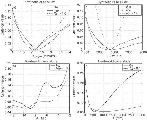
differ-ence of the identified best simulations under all three calibra-tion criteria is, however, hardly detectable. There is, nonethe-less, an interesting difference: the optimum parameter values under the two frequency-domain criteria are clearly much better defined than under RN (Fig. 3a and b). This holds
in particular for the least sensitive parameter, the nonlinear direct runoff parameter β. It is noteworthy, however, that this does not indicate a better identifiability in the wavelet-domain in general but depends on the chosen formulation of the time-domain objective function (for a discussion of the shape of time-domain objective functions, refer to Beven and Freer, 2001).
5.1.3 Experiment 3
If we try to estimate the model parameters on a reference series that was generated with a different model structure, i.e. with a variable degree-day factor for snowmelt, the per-formances underRN andRW are very close but each of the
criteria lead to distinct solutions for the constant degree-day factor (Table 4), both of which lead to good simulations. The two solutions are hardly distinguishable based on the used performance measures (Table 4) and are very close to the generated reference series (see Fig. 4). A look on the average wavelet-power over certain ranges of scales, however, clearly shows that the simulations having a constant degree-day fac-tor do not reproduce the true dynamics (Fig. 4), neither for the best parameter set in the time-domain nor for the best parameter set in the wavelet-domain.
5.2 Real-world case study
5.2.1 Parameter estimation in the wavelet-domain versus in the time-domain
There is certain trade-off between the time-domain and the wavelet-domain objective function. The optimum for RN
does not correspond to the optimum for RW (Table 5). It
is noteworthy that for this case study, the apparently high Nash values (0.94 for the best simulation under RN, 0.91
under RW) do not necessarily mean that the hydrological
model does a particularly good job, high Nash values are easy to achieve for times series with a strong annual cycle (see Schaefli and Gupta, 2007).
At a first glance, the optimal parameter sets do not seem to be fundamentally different underRN and underRW (see
Table 5). A closer look shows however some notable dif-ferences. Even if physically meaningless parameter sets are penalized, the optimization underRN leads to a global
1000 3000 5000 7000 9000 0
0.02 0.04 0.06 0.08 0.10 0.12 0.14
β (m4/3 /s)
Criterion value
RN RW
RF - 1.6
Synthetic case study
b)
c) d)
Real-world case study Real-world case study
-12 -10 -8 -6 -4 -2 0.04
0.06 0.08 0.10 0.12 0.14 0.16 0.18 0.20 0.22
lk (1/h)
0 500 1000 1500 2000 2500 3000 0.05
0.10 0.15 0.20 0.25 0.30
A (mm) RN RW - 0.1 RN
RW - 0.1 1 1.5 2 2.5 3 3.5 4 0
0.02 0.04 0.06 0.08 0.10 0.12 0.14
asnow (mm/d/°C)
Criterion value
RN RW
RF - 1.6 a)
Synthetic case study
Criterion value
Criterion value
Criterion value
c) d)
Fig. 3.Parameter sensitivity around the optimum value identified under the different calibration criteria; top: experiment 2, the most sensitive parameterasnow(a), and the least sensitive parameterβ(b), the other parameters are kept constant to the values of Table 3; bottom: real-world
case study, the two least sensitive parameterslk(c)andA(d), the other parameters are kept constant to the values of Table 5.
100 200 300 400 500 600 700 800 900 1000
0 5 10 15
Time step (days)
Discharge mm/d
100 200 300 400 500 600 700 800 900 1000
0 0.1 0.2
Power
Average wavelet power of scales 16 to 64 days
Reference series
Calibrated with RW
Reference series
Calibrated with RN
Calibrated with RW
Time step (days) Discharge time series
Fig. 4. Experiment 3, top: reference and calibrated discharge underRW (calibrated discharge underRN is almost identical and, thus, not
0 5 10 15 20 25 30 35
Time step (d)
Discharge (mm/d)
Observed discharge Calibrated with RN
23/06/86 28/07/87 31/08/88 05/10/89 09/11/90 14/12/91 0.005
0.010 0.015 0.020 0.025
Av. power of scales 128 to 256 days
Observed discharge Calibrated with RN Calibrated with RW
24/01/86 15/03 04/05 23/06 12/08 01/10 20/11/86 0
5 10 15 20 25 30 35
Date
Discharge (mm/d)
Observed discharge Calibrated with RW a)
b)
c)
24/01/86 15/03 04/05 23/06 12/08 01/10 20/11/86 Date
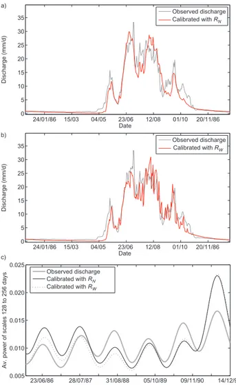
Fig. 5.Real-world case study:(a)zoom on the observed discharge for the year 1986 (calibration period) and the simulation calibrated underRN;(b)as (a) but simulation calibrated underRW;(c)zoom
on the average estimated wavelet-power between the scales of 128 days and 256 days for the observed discharge and the simulations calibrated underRW, respectively underRN.
In addition, the parameters have (as for the synthetic case study) a better identified optimum underRW than underRN,
especially for the parameters with the lowest sensitivity, the soil transfer parameters (Fig. 3c and d).
Close inspection of the discharge simulations based on the best parameters obtained in the time-domain and in the wavelet-domain, respectively, shows that both parame-ter sets yield rather different discharge dynamics (see zooms on the simulations in Fig. 5 and scatter-plots of observed against simulated discharge in Fig. 6). Without further cross-validation data (e.g. observed ice melt data), it is difficult to judge which parameter set captures the observed dynamics better. An interesting hint is, however, given by the follow-ing analysis: we build a prediction interval based on 90 of the 100 best random simulations. UnderRN, this interval
in-0 5 10 15 20 25 30 35 40 45
0 5 10 15 20 25 30 35 40 45
Simulated discharge (mm/day)
Observed discharge (mm/day)
Calibrated with RW
Calibrated with RN
Model performance - entire period
Fig. 6. Real-world case study: scatter-plot of observed discharge (during calibration period) against best simulation under each of the two calibration criteria.
Table 2. Parameter intervals delimiting the search space for the real-world case study and for the synthetic experiments 2 and 3; pa-rameter sets that do not respect the imposed physical conditions are penalized during parameter set evaluation (for more details about these parameters, see Schaefli et al., 2005).
Parameter Unit Min Max Significance Condition/penalty
aice mm/d/◦C 1.0 16.0 Degree factors for ice resp. snow
aice>asnow
penalty =asnow−aice asnow mm/d/◦C 0.5 12.0
kice d 0.5 45.0 Linear reservoir coeffi-cient for ice resp. snow melt
kice<ksnow
penalty=(kice−ksnow)/2
ksnow d 1.0 45.0
A mm 1 3000 Max. storage for linear slow response reservoir
lk log(1/h) −12.0 −0.1 Coeff. for linear slow re-sponse
β m4/3/s 1 30 000 Coeff. for nonlinear, fast
response
Tcrit ◦C 1.0 1.0 Threshold for snowfall Fixed
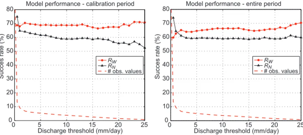
cludes around 80% of all observations for the calibration pe-riod. This success rate decreases constantly if we evaluate it for discharges above a certain threshold (Fig. 7). ForRW, the
success rate, which is overall slightly lower than underRN,
remains constant for all discharge thresholds. This clearly suggests that for this case study, good simulations in the wavelet-domain capture equally well all discharge ranges. Good simulations under RN, however, capture particularly
0 5 10 15 20 25 0
10 20 30 40 50 60 70 80
Succes rate (%)
Discharge threshold (mm/day) RW
RN # obs. values
0 5 10 15 20 25
0 10 20 30 40 50 60 70 80
Succes rate (%)
Discharge threshold (mm/day) Model performance - entire period Model performance - calibration period
RW
RN # obs. values
Fig. 7. Real-world case study: model performance for the best 100 random simulations (of 20 000 random parameter sets) under RW, respectivelyRN; the success rate measures the relative number of observed daily discharges above a certain threshold that fall within the
90% prediction range of the retained 100 simulations; left calibration period, right entire period.
Table 3.Experiment 2: parameter values used to generate the syn-thetic discharge time series and the identified optimal parameters sets underRW,RF andRN; the glacier surface is set to 0, which
eliminates the parametersaice,kiceandksnow; calib: calibration
pe-riod; valid: validation pepe-riod; for other abbreviations, see Table 1.
CalibrationRW CalibrationRN CalibrationRF
Parameter/criterion Exact Calib Valid Calib Valid Calib Valid
asnow 2.2 2.2 2.2 2.2
A 550 691 544 557
log(k) −9.1 −9.6 −9.1 −9.1
β 4500 4748 4546 4478 corr pert 0.97 0.97 0.96 0.97 0.97 0.97 0.97
RWpert 0.15 0.14 0.15 0.15 0.15 0.15 0.15
RFpert −1.01 −0.84 −0.37 −0.85 −0.38 −0.85 −0.38
LNpert 0.94 0.93 0.92 0.94 0.93 0.94 0.93
corr unpert 1 1.00 1.00 1.00 1.00 1.00 1.00
RWunpert 0 0.04 0.05 0.00 0.00 0.00 0.00
RFunpert NaN −1.44 −0.95 −1.51 −0.98 −1.51 −0.98
LNunpert 1 0.99 0.99 1.00 1.00 1.00 1.00
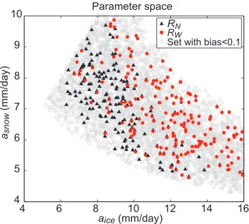
The above results suggest an important difference between the best parameter sets in the time-domain and the best pa-rameter sets in the wavelet-domain. A look on the papa-rameter space of the most sensitive parameters, the degree-day fac-tors for snowmelt (asnow) and for ice melt (aice) illustrates
this difference: Fig. 8 shows a scatter-plot ofasnow against aicefor all “physically feasible” parameter sets, i.e.
parame-ter sets that lead to a bias smaller than 10% (the visible de-pendance between physically feasible snow and ice melt fac-tors is a common result for this type of models, see Schaefli et al., 2005). The 100 parameter sets that, among all physi-cally feasible parameter sets, have the lowestRW values are
highlighted in red; the parameter sets with the lowestRN
val-ues are highlighted as triangles. These two groups show that the best parameter sets underRNcorrespond to another area
of the physically feasible parameter space than the best pa-rameter sets underRW. Retaining good solutions under the
Table 4. Experiment 3: parameters used to generate the synthetic reference discharge time series and the identified optimal parame-ters values using theRW andRN performance criteria; the
refer-ence time series has been generated using a variableasnow
parame-ter throughout the year; theasnowparameter values for each month
are{1.2, 1.4, 1.4, 2.0, 4.0, 5.0, 6.0, 7.0, 5.0, 2.0, 1.2 , 1.1}; for abbreviations see Table 1.
Parameter Exact RW RN
asnow variable 2.2 2.4
A 550 584 438
lk −9.1 −9.5 −8.7
β 4500 4180 4731
ksnow 15.6 29.1 24.8
corr 1 0.94 0.95
RW 0 0.08 0.09
LN 1 0.88 0.90
quadratic error-based criteria RN further reduces the
phys-ically feasible parameter space. In contrast, the group of the best parameter sets underRW appears to show the same
dependance betweenasnow andaice as the overall group of
physically feasible parameter sets. This result suggests that:
1. The bias criterion could be sufficient to ensure solu-tions that reproduce the dominant frequencies (which is a very interesting result for snow- and ice melt mod-eling).
2. TheRN could be too restrictive and exclude solutions
that can reproduce the frequency content of the ob-served time series. This means that for this particu-lar case study, a parameter estimation based on theRN
This last hypothesis is supported by the fact thatRN only
leads to unbiased parameter estimates if the model residuals are Gaussian with a constant variance (for a discussion, see Kavetski et al., 2006a). For the present case study, the resid-uals clearly have a different variance during the summer and the winter season (see Schaefli et al., 2006).
5.2.2 Model diagnostics
A visual inspection of the average wavelet-power at bands of scales ranging from weeks to a few months shows that even the best models do not well capture the observed dy-namics (see an example in Fig. 5c): both best models (under
RW andRN)do not well reproduce the frequency content
of the observed series. The models have a somewhat differ-ent behavior but the plot of the average power at high scales suggests that given the observed input and the current model structure, the model cannot produce a closer fit to the esti-mated wavelet-power of the observed series. The power con-tent tends to be either largely over- or underestimated.
The model’s inability to reproduce the frequency content at high scales (months) suggests that either a storage term is missing or is not well parameterized in the current model structure. In fact, the model does not simulate separately the melt and the transfer of firn, i.e. of old snow that lasts more than one season and that is a transition state between ice and snow. Firn has a degree-day factor and melt water transfer times that are between the ones of ice and of snow (e.g. Klok et al., 2001) and induces a further partitioning of the discharge during the melt season. Its contribution to the total discharge depends on the annual snowfall.
The mismatch of the calibrated and observed wavelet pe-riodograms at intermediate scales (weeks) could be a hint that the model does not fully capture the relationship be-tween temperature and snow- and ice melt. This relation-ship is constant in the current model parameterization but it is known to be variable throughout the melt season (for ex-ample due to changes in the albedo, see, e.g. Rango and Mar-tinec, 1995). But the models’ inability to reproduce these scales could also indicate the need to improve the meltwa-ter transfer through the glacier and the overlaying snowpack. In the model, this transfer is encoded by a linear transfer function having a constant parameter. In reality, the trans-fer of melt water through a glacier is highly variable in time since the glacier drainage system evolves throughout the melt season (see, e.g. Willis, 2005). In warm years, it develops and evacuates water much faster than during cold years. A detailed analysis of the wavelet-power at different bands of the observed and the simulated time series during years with high snowfall and low snowfall, respectively during cold and warm years could help gaining further insights into which of the above model structural deficiencies are more important.
4 6 8 10 12 14 16
4 5 6 7 8 9 10
aice (mm/day)
asnow
(mm/day)
RN RW
Set with bias<0.1 Parameter space
Fig. 8.Real-world case study: relationship betweenasnowandaice
for the 100 best parameters sets (of 20 000 random parameter sets) underRN, respectively underRW.
Table 5.Real-world case study: optimal parameter values identified using global optimization andRW andRNas objective-functions;
calib=calibration period, valid=validation period, var. bias=relative difference between variance of observed and simulated time series.
RW RN
aice 8.5 7.8
asnow 6.8 8.2
lk −8.8 −9.7
A 539 1014
β 6279 274
kice 1.5 2.1
ksnow 37.0 26.0
RW calib 0.086 0.088
RW valid 0.087 0.090
LNcalib 0.91 0.94
LNvalid 0.91 0.93
B −0.06 −0.05
Var. bias −0.09 −0.04
5.3 Computational costs
The computation of the wavelet-domain performance crite-rion involves first of all the computation of the wavelet pe-riodogram of the analyzed time series, which requires con-volving the signal (observed or simulated times series) with the wavelet at each scale. This implies a number of in-verse Fast Fourier Transforms that equals the number of an-alyzed scales. This “pre-treatment” of the time series before the computation of the performance criterion increases the computational cost by a factor at least equal to the num-ber of scales. The Kolmogorov -Smirnov distance-based performance criterion also involves more calculations than the computation of a squared error-based distance measure. In our case, using a Matlab® code on a laptop with a Intel®Pentium® M 1.5 GHz processor, the computation of the inverse Fast Fourier Transform for one scale is roughly twice longer than the computation of a Nash criterion over the entire time series. For a time series with 6939 time steps, computing the Nash efficiency takes typically 0.01 s whereas computing the wavelet periodogram for 122 scales takes 1.9 s and computing the Kolmogorov-Smirnov distance takes an-other 0.6 s.
6 Conclusions and outlook
The present paper discusses and illustrates parameter estima-tion and model performance analysis of rainfall-runoff mod-els in the wavelet-domain with the main purpose to show how this could contribute to hydrological model diagnostics and to model structure improvement.
As discussed based on theoretical considerations and based on the presented examples, parameter estimation for at least partly misspecified models in the wavelet-domain can yield different results than parameter estimation in the time-domain. Especially for observed time series having a strongly time-varying frequency content, the suggested ap-proach allows estimation of model parameter sets in the wavelet-domain that are internally consistent and allow sim-ulations with more plausible dynamics than a parameter esti-mation in the time-domain. However, it is at the current stage difficult to determine a priori in which cases a calibration in the wavelet-domain could yield better representations of the true system dynamics. Future case studies and theoretical developments should provide insights into this question. A key hereby will be the detailed study of the behavior of the wavelet-domain performance criterion in presence of errors in the input or output data.
In general, a detailed investigation of the origin of the dif-ferences between the best solutions in the wavelet-domain and in the time-domain can offer additional and new pieces to the puzzle of understanding conceptual model behavior and shortcomings. For the real-world case study presented in this paper, the best parameter sets in the wavelet-domain do
for example not show the same dependence structure as the best parameter sets in the time-domain. Such a result is a hint that the model has structural deficiencies. These deficiencies can then be further investigated by analyzing in detail how the model performs over relevant ranges of temporal scales, by visually inspecting the power content of the wavelet pe-riodograms or by computing wavelet performance measures over certain scales instead of over the entire range of resolv-able scales. As illustrated for the real-world case study, this can give valuable indications on model deficiencies and how to overcome them.
Just as different objective functions can be formulated in the time-domain, the presented wavelet-based criterion corresponds to one possible performance measure in the wavelet-domain. Other formulations (and other wavelets) are possible and would potentially yield other optimal param-eter sets. While the statistical properties of different time-domain objective functions are well understood, applications of wavelet spectral analysis to geosciences are still relatively recent and statistical questions have to be further evaluated. We would thus like to emphasize that the potential of param-eter estimation in the wavelet-domain lies in the information that it yields for model improvement.
For very long time series, the computational cost for the evaluation of the wavelet criterion can become important. This aspect is however counterbalanced by the gained in-sights. We are confident that future case studies including namely not only discharge data but also other sources of validation data will provide additional evidence for the po-tential of parameter estimation and model diagnostics in the wavelet-domain.
A Matlab® code for the computation of the presented per-formance measure can be obtained from the first author.
Acknowledgements. The research of the first author was funded by Fellowships of the Swiss National Science Foundation and of the German National Science Foundation. Our Matlab code is based on a code originally written by C. Torrence and G. Compo that is available at http://paos.colorado.edu/research/wavelets/. The code for the IAFFT algorithm has been written by V. Venema and is available at http://www.meteo.uni-bonn.de/mitarbeiter/venema. The meteorological time series have been provided by the Swiss Meteorological Institute MeteoSwiss and the hydrological time series by the Hydrological Section of the Swiss Federal Office for the Environment. We also would like to thank the anonymous reviewers for their detailed suggestions to improve the paper structure.
Edited by: E. Todini
References
Bl¨oschl, G. and Zehe, E.: Invited commentary – On hydrological predictability, Hydrol. Process., 19, 3923–3929, 2005.
Boyle, D. P.: Multicriteria calibration of hydrological models, De-partment of Hydrology and Water Resources, University of Ari-zona, Tucson, 193 pp., 2000.
Contreras-Crist´an, A., Guti´errez-Pe˜na, E., and Walker, S. G.: A Note on Whittle’s Likelihood, Commun. Stat.-Simul. C., 35, 857–875, 2006.
Daubechies, I.: Ten Lectures on Wavelets, Society for Industrial and Applied Mathematics, Philadelphia, Pennsylvania, 357 pp., 1992.
Frei, C. and Sch¨ar, C.: Detection probability of trends in rare events: Theory and application to heavy precipitation in the Alpine re-gion, J. Climate, 14, 1568–1584, 2001.
Gabor, D.: Theory of communication, J. IEE, 93, 429–457, 1946. Gaucherel, C.: Use of wavelet transform for temporal
characterisa-tion of remote watersheds, J. Hydrol., 269, 101–121, 2002. Grossmann, A. and Morlet, J.: Decomposition of Hardy functions
into square integrable wavelet constant shape, SIAM J. Math. Anal., 15, 723–736, 1984.
Gupta, H. V., Beven, K. J., and Wagener, T.: Model Calibration and Uncertainty Estimation, in: Encyclopedia of Hydrological Sciences, edited by: Anderson, M. G., Wiley, Chichester, UK, 2015–2032, 2005.
Hannan, E. J.: The asymptotic theory of linear time-series models, J. Appl. Prob., 10, 130–145, 1973.
Herbst, M. and Casper, M. C.: Towards model evaluation and iden-tification using Self-Organizing Maps, Hydrol. Earth Syst. Sci., 12, 657–667, 2008,
http://www.hydrol-earth-syst-sci.net/12/657/2008/.
Herren, E. R., Bauder, A., Hoelzle, M., and Maisch, M.: The Swiss Glaciers 1999/2000 and 2001/2002, Glaciological Commission of the Swiss Academy of Sciences, Z¨urich, Glaciological Report 121/122, 73, 2002.
Hock, R.: Temperature index melt modelling in mountain areas, J. Hydrol., 282, 104–115, 2003.
Holschneider, M.: Wavelets: an analysis tool, Oxford University Press, Oxford, UK, 423 pp., 1998.
Kaiser, G.: A friendly Guide to Wavelets, Birkh¨auser, New York, USA, 300 pp., 1994.
Kavetski, D., Kuczera, G., and Franks, S. W.: Bayesian analysis of input uncertainty in hydrological modeling: 1. Theory, Water Resour. Res., 42, W03407, doi:10.1029/2005WR004368, 2006a. Kavetski, D., Kuczera, G., and Franks, S. W.: Calibration of con-ceptual hydrological models revisited: 1. Overcoming numerical artefacts, J. Hydrol., 320, 173–186, 2006b.
Klok, E. J., Jasper, K., Roelofsma, K. P., Gurtz, J., and Badoux, A.: Distributed hydrological modelling of a heavily glaciated Alpine river basin, Hydrol. Sci. J., 46, 553–570, 2001.
Labat, D.: Recent advances in wavelet analyses: Part 1. A review of concepts, J. Hydrol., 314, 275–288, 2005.
Lafreni`ere, M. and Sharp, M.: Wavelet analysis of inter-annual vari-ability in the runoff regimes of glacial and nival stream catch-ments, Bow Lake, Alberta, Hydrol. Process., 17, 1093–1118, 2003.
Lane, S. N.: Assessment of rainfall-runoff models based upon wavelet analysis, Hydrol. Processes, 21, 586–607, 2006. Leyland, G. B.: Multi-Objective Optimisation Applied to Industrial
Energy Problems, Laboratoire d’Energ´etique Industrielle, Ecole
Polytechnique F´ed´erale de Lausanne, Switzerland, available at: http://library.epfl.ch/theses, 188 pp., 2002.
Maraun, D. and Kurths, J.: Cross wavelet analysis: significance testing and pitfalls, Nonlin. Processes Geophys., 11, 505–514, 2004,
http://www.nonlin-processes-geophys.net/11/505/2004/. Maraun, D., Kurths, J., and Holschneider, M.: Non-stationary
Gaussian Processes in Wavelet Domain: Definitions, Esti-mation and Significance Testing, Phys. Rev. E, 75, 016707, doi:10.1103/PhysRevE.75.016707, 2007.
Montanari, A. and Toth, E.: Calibration of hydrological models in the spectral domain: an opportunity for ungauged basins?, Water Resour. Res., 43, W05434, doi:10.1029/2006WR005184, 2007. Moulines, E., Roueff, F., and Taqqu, M. S.: A wavelet Whittle
es-timator of the memory parameter of a non-stationary Gaussian time series, Ann. Stat., 36, 1925–1956, 2008.
Nash, J. E. and Sutcliffe, J. V.: River flow forecasting through con-ceptual models. Part I, a discussion of principles, J. Hydrol., 10, 282–290, 1970.
Nic´otina, L., Alessi Celegon, E., Rinaldo, A., and Marani, M.: On the impact of rainfall patterns on the hydrologic response, Water Resour. Res., 44, W12401, doi:10.1029/2007WR006654, 2008. Priestley, M.: Spectral Analysis and Time Series, Academic Press,
London, UK, 884 pp., 1981.
Rango, A. and Martinec, J.: Revisiting the degree-day method for snowmelt computations, Water Resour. Bull., 31, 657–669, 1995. Reusser, D. E., Blume, T., Schaefli, B., and Zehe, E.: Analysing the temporal dynamics of model performance for hydrological models, Hydrol. Earth Syst. Sci. Discuss., 5, 3169–3211, 2008, http://www.hydrol-earth-syst-sci-discuss.net/5/3169/2008/. Schaefli, B., Hingray, B., and Musy, A.: Improved calibration of
hydrological models: use of a multi-objective evolutionary algo-rithm for parameter and model structure uncertainty estimation, Hydrology: Science and Practice for the 21st Century, London, UK, 362–371, 2004.
Schaefli, B.: Quantification of modelling uncertainties in climate change impact studies on water resources: Application to a glacier-fed hydropower production system in the Swiss Alps, Ecole Polytechnique F´ed´erale de Lausanne, Switzerland, avail-able at: http://library.epfl.ch/theses, 209 pp., 2005.
Schaefli, B., Hingray, B., Niggli, M., and Musy, A.: A con-ceptual glacio-hydrological model for high mountainous catch-ments, Hydrol. Earth Syst. Sci., 9, 95–109, 2005,
http://www.hydrol-earth-syst-sci.net/9/95/2005/.
Schaefli, B., Balin Talamba, D., and Musy, A.: Quantifying hy-drological modeling errors through a mixture of normal distribu-tions, J. Hydrol., 332, 303–315, 2006.
Schaefli, B. and Gupta, H.: Do Nash values have value?, Hydrol. Process., 21, 2075–2080, 2007.
Schaefli, B., Maraun, D., and Holschneider, M.: What
drives high flow events in the Swiss Alps? Recent de-velopments in wavelet spectral analysis and their applica-tion to hydrology, Adv. Water Resour., 30(12), 2511–2525, doi:10.1016/j.advwatres.2007.06.004, 2008
Schaefli, B. and Zehe, E.: Hydrological model performance and parameter estimation in the wavelet-domain, Hydrol. Earth Syst. Sci. Disc., 6, 2451–2498, 2009.
Climatol., 25, 753–771, 2005.
Schreiber, T. and Schmitz, A.: Surrogate time series, Physica D, 142, 346–382, 2000.
Shumway, R. H. and Stoffer, D. S.: Time Series Analysis and Its Applications, With R Examples, 2nd edn., Springer, New York, USA, 576 pp., 2006.
Si, B. C. and Zeleke, T. B.: Wavelet coherency analysis to relate saturated hydraulic properties to soil physical properties, Water Resour. Res., 41, W11424, doi:10.1029/2005WR004118, 2005. Torrence, C. and Compo, G. P.: A practical guide to wavelet
analy-sis, B. Am. Meteorol. Soc., 79, 61–78, 1998.
Velasco, C.: Gaussian semiparametric estimation of non-stationary time series, J. Time Ser. Anal., 20, 87–127, 1999.
Vrugt, J. A., Gupta, H. V., Bouten, W., and Sorooshian, S.: A shuf-fled complex evolution Metropolis algorithm for optimization and uncertainty assessment of hydrologic models, Water Resour. Res., 39, 1201, doi:10.1029/2002WR001642, 2003.
Wagener, T., Boyle, D. P., Lees, M. J., Wheater, H. S., Gupta, H. V., and Sorooshian, S.: A framework for development and applica-tion of hydrological models, Hydrol. Earth Syst. Sci., 5, 13–26, 2001,
http://www.hydrol-earth-syst-sci.net/5/13/2001/.
Weisstein, E. W.: Metric, From MathWorld-A Wolfram Web Re-source, http://mathworld.wolfram.com/Metric.html, last access: 19 March 2009, 2009.
Whittle, P.: Estimation and information in stationary time series, Ark. Mat., 2, 423–434, 1953.
Willis, I.: Hydrology of glacierized basins, in: Encyclopedia of Hy-drological Sciences, edited by: Anderson, M. G., Wiley, Chich-ester, UK, 2601–2631, 2005.
Winsemius, H., Schaefli, B., Montanari, A., and Savenije, H. H. G.: On the calibration of hydrological models in ungauged basins: a framework for integrating hard and soft hydrological informa-tion, Water Resour. Res., doi:10.1029/2009WR007706, in press, 2009.
Yao, Q. and Brockwell, P. J.: Gaussian Maximum Likelihood Es-timation For ARMA Models. I. Time Series, J. Time Ser. Anal., 27, 857–875, 2006.
Yilmaz, K. K., Gupta, H. V., and Wagener, T.: A process-based di-agnostic approach to model evaluation: Application to the NWS distributed hydrologic model, Water Resour. Res., 44, W09417, doi:10.1029/2007WR006716, 2008.
Zehe, E., Becker, R., Bardossy, A., and Plate, E.: Uncertainty of simulated catchment runoff response in the presence of thresh-old processes: Role of initial soil moisture and precipitation, J. Hydrol., 315, 183–202, 2005.