Analysis of the proficiency of fully-connected neural networks in the process of classifying digital images : benchmark of different classification algorithms on high-level image features from convolutional layers

(1)

Jonathan Gabriel Martin Janke

Benchmark of Different Classification Algorithms

on High-Level Image Features from

Convolutional Layers

Dissertation presented as partial requirement for

obtaining the

Master’s degree in Advanced Analytics

ANALYSIS OF THE PROFICIENCY OF  

FULLY-CONNECTED NEURAL NETWORKS IN THE

PROCESS OF CLASSIFYING DIGITAL IMAGES

(2)

 

(3)

(4)

ANALYSIS OF THE PROFICIENCY OF  

FULLY-CONNECTED NEURAL NETWORKS IN THE  

PROCESS OF CLASSIFYING DIGITAL IMAGES

by

Jonathan Gabriel Martin Janke

Dissertation presented as partial requirement for obtaining the Master’s degree in Advanced Analytics

Advisor: Mauro Castelli

(5)

(6)

The NOVA Information Management School and the NOVA University Lisbon have the right, perpetual and without geographical boundaries, to file and publish this dissertation through printed copies reproduced on paper or on digital form, or by any other means known or that may be invented, and to disseminate through scientific repositories and admit its copying and distribution for non-commercial, educational or research purposes, as long as credit is given to the author and editor.

This document was created using the (pdf)LA_{TEX processor, based in the “novathesis” template[1], developed at the Dep. Informática of FCT-NOVA [2].}

(7)

(8)

I appreciate the various discussions I had with di↵erent people from my faculty from the ideation phase to the execution and the interpretation of the final results. I would like to thank everybody that took their time to listen to my ideas, help me fine-tune the thesis and shape it to what it is now. Furthermore, I am grateful for everybody that read my thesis and provided me with feedback. This also goes for the people that helped me write an abstract in Portuguese.

I also want to thank my supervisor Mauro Castelli for giving me the necessary support and feedback during the thesis. I am thankful for the freedom I had when choosing the topic that I want to do research on and the timeline to realise the thesis.

Further appreciation goes to Thaís Góes for the support and all the help during the thesis. Thanks to everybody else who accompanied me on my journey. It feels good to have people around you that support you and that you can rely on.

Lastly, I would like to thank my family, in particular my parents, Stephanie and Martin Janke. Thank you for the trust that you have put into me and my personal development and the liberty that you have given me during my studies. I appreciate all the support I have received during my Bachelor’s and Master’s degree that enabled me to fully focus on those.

(9)

(10)

Over the course of research on Convolutional Neural Network (CNN) architectures, little modifications have been done to the fully-connected layers at the end of the net-works. In image classification, these neural network layers are responsible for creating the final classification results based on the output of the last layer of high-level image filters. Before the breakthrough of CNNs, these image filters were handcrafted, and any classification algorithm was applied to their output. Because neural networks use gradients to learn their weights subject to the classification error, fully-connected neural networks are a natural choice for CNNs. But the question arises: Are fully-connected layers in a CNN superior to other classification algorithms? After the net-work is trained, the approach is to benchmark di↵erent classification algorithms on CNNs by removing the existing fully-connected classifier. Thus, the flattened output from the last convolutional layer is used as the input for multiple benchmark classi-fication algorithms. To ensure the generalisability of the findings, numerous CNNs are trained on CIFAR-10, CIFAR-100 and a subset of ILSVRC-2012 with 100 classes. The experimental results reveal that multiple classification algorithms are capable of outperforming fully-connected neural networks in di↵erent situations, namely Logis-tic Regression, Support Vector Machines, eXtreme Gradient Boosting, Random Forests and K-Nearest Neighbours. Furthermore, the superiority of individual classification algorithms depends on the underlying CNN structure and the nature of the classifi-cation problem. For classificlassifi-cation problems with multiple classes or for CNNs that produce many high-level image features, other classification algorithms are likely to perform better than fully-connected neural networks. It follows that it is advisable to benchmark multiple classification algorithms on high-level image features produced from the CNN layers to improve performance or model size.

Keywords: Convolutional Neural Networks, CNN, Neural Networks, Computer Vi-sion, Image Classification, Image Features, CIFAR-10, CIFAR-100, ILSVRC-2012

(11)

(12)

Desde a criação da arquitetura da Rede Neural Convolucional (CNN), poucas modifi-cações foram feitas nas camadas totalmente conectadas (fully-connected) no final das redes. Na classificação de imagens, estas mesmas camadas são responsáveis por criar os resultados finais da classificação, com base no output da última camada de filtros de imagem de alto nível (high-level image filters). Antes do avanço das CNNs, estes filtros de imagem eram feitos à mão e qualquer algoritmo de classificação era apli-cado ao seu output. Como as redes neuronais aprendem os seus pesos gradualmente com gradientes sujeitos a um erro, as redes neuronais totalmente conectadas são uma escolha natural para as CNNs. No entanto, a superioridade das camadas totalmente conectadas numa CNN em relação a outros algoritmos de classificação é contestada. Depois da rede neural ser treinada, a abordagem passa por comparar diferentes algorit-mos de classificação em CNNs, removendo o atual classificador totalmente conectado. Deste modo, o output achatado (flattened output) da última camada convolucional é usado como input para vários algoritmos de benchmarking. Para assegurar a genera-lização dos resultados, várias CNNs são treinadas no CIFAR-10, no CIFAR-100 e num subconjunto do ILSVRC-2012. Os resultados experimentais revelam que múltiplos algoritmos são capazes de superar redes neuronais totalmente conectadas, nomeada-mente Regressão Logística, Support Vector Machines, XG Boosting, Random Forests e K-Nearest Neighbours. Além disso, a superioridade de cada algoritmo depende da es-trutura subjacente da CNN e da natureza do problema de classificação. Para problemas com várias classes de output ou para CNNs que produzem muitos recursos de imagem de alto nível, outros algoritmos de classificação provavelmente terão um desempenho melhor do que redes neuronais totalmente conectadas. Segue-se que é aconselhável comparar vários algoritmos em recursos de imagem de alto nível produzidos a partir das camadas da CNN, para melhorar o desempenho ou o tamanho do modelo.

(13)

(14)

List of Figures xiii

List of Tables xv

1 Introduction 1

1.1 Background Information . . . 1

1.2 Structure of the Thesis . . . 3

1.3 Purpose of the Thesis . . . 3

2 Artificial Neural Networks for Computer Vision 5 2.1 How are Digital Images Represented . . . 6

2.2 Challenges in Computer Vision . . . 6

2.3 Convolutional Neural Networks . . . 7

2.3.1 Convolutional Layers . . . 9

2.3.2 Depthwise Separable Convolutions . . . 13

2.3.3 Pooling Layers . . . 15

2.3.4 Fully-Connected Layers . . . 15

2.3.5 Dropout Layer . . . 16

2.3.6 Batch Normalisation Layers . . . 17

2.3.7 Inception Modules . . . 18

2.3.8 Residual Blocks . . . 22

2.3.9 Capsules . . . 23

2.3.10 Transfer Learning . . . 27

3 Classification in Supervised Environments 29 3.1 Decision Trees . . . 30

3.2 Ensemble Methods . . . 33

3.2.1 Random Forest Classifier. . . 35

3.2.2 Adaptive Boost Classifier. . . 36

3.2.3 Gradient Boosting Classifier . . . 36

3.2.4 eXtreme Gradient Boosting Classifier . . . 39

3.3 Logistic Regression . . . 41

(15)

3.5 K-Nearest Neighbours . . . 45

3.6 Multi-Layer Perceptrons . . . 46

3.7 Classification Evaluation Methods . . . 47

3.7.1 Accuracy . . . 48

3.7.2 Top-n Accuracy . . . 49

3.7.3 Confusion Matrices . . . 49

3.7.4 Precision, Recall and FnMeasure . . . 50

3.7.5 ROC AUC Score . . . 52

3.7.6 Model Speed . . . 53 4 Experimental Setup 55 4.1 Work References . . . 56 4.2 Scientific Procedure . . . 56 4.3 Dataset Benchmarks. . . 59 4.3.1 CIFAR-10 . . . 59 4.3.2 CIFAR-100 . . . 61

4.3.3 ImageNet Large Scale Visual Recognition Challenge 2012 . . . 62

4.4 Model Architecture Benchmarks. . . 63

4.4.1 ILSVRC-2012 Architecture Benchmarks . . . 65

4.4.2 CIFAR Architecture Benchmarks . . . 66

4.5 Image Preprocessing . . . 68

4.6 Classification Algorithms Used . . . 74

4.7 Selection of Evaluation Metrics . . . 77

4.8 Software Architecture of the Final Solution . . . 78

5 Experimental Evaluation 79 5.1 Output from Convolutional Neural Network Structures . . . 80

5.1.1 CIFAR-10 Intermediate Observations . . . 80

5.1.2 CIFAR-100 Intermediate Observations . . . 82

5.1.3 ILSVRC-2012 Subset Intermediate Observations . . . 84

5.2 MLP Architecture Comparison on Intermediate Datasets . . . 85

5.3 Comparing Di↵erent Classification Algorithms on Image Features . . 90

5.3.1 CIFAR-10 Results . . . 91

5.3.2 CIFAR-100 Results . . . 95

5.3.3 ILSVRC-2012 Results . . . 99

5.4 Interpretation of Results . . . 103

5.5 Conclusion of Results . . . 106

6 Conclusion and Outlook 109 6.1 Conclusion . . . 109

(16)

Bibliography 115

A Appendix 125

A.1 Convolutional Neural Networks . . . 125

A.1.1 Exemplification of Computer Vision challenges . . . 125

A.1.2 Reformulation and simplification of Inception Module Formula 128 A.1.3 Visualisation of general architecture of CNN . . . 128

A.2 Experimental datasets. . . 129

A.2.1 Normalised images from CIFAR-10 . . . 129

A.2.2 Image classes from CIFAR-100 . . . 130

A.2.3 Normalised images from CIFAR-100 . . . 136

A.2.4 100 classes used from ILSVRC-2012 . . . 142

A.3 Classification results . . . 148

A.3.1 CIFAR-10 . . . 148

A.3.2 CIFAR-100 . . . 156

(17)

(18)

11 Summary of Di↵erent Computer Vision Tasks from [91] . . . 2

21 LeNet-5 Architecture from LeCun et al. (1998) . . . 8

22 Application of convolutional layer with n image filters of size kw⇥ kh⇥ 3 with stride s = 1 on input data with size widthw ⇥ height h and an input depth of 3 [99] . . . 9

23 _{Visualisation of application of a linear k ⇥ k ⇥ 1 image filter on receptive} field in input [99] . . . 11

24 Simple Inception Module, modified from Szegedy et al. (2014) [95]. . . . 18

25 Advanced Inception Module designed to reduce the overall complexity, modified from Szegedy et al. (2014) [95] . . . 20

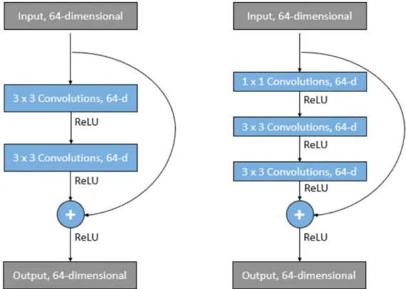
26 Two example residual block architectures, modified from He et al. (2015) [31] 22 27 A convolutional neural network does not e↵ectively capture the spatial relationship among concepts but simply detects the existance of certain elements . . . 23

28 Exemplified vector creation from convolutional layers . . . 25

29 Example of a MECE solution in a multi-label classification task from [10] 26 31 General Classification Procedure from [98]: p. 146 . . . 29

32 Illustration of a Decision Tree creation process using Hunt’s algorithm from [98], p. 154. . . 31

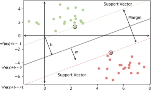
33 Explanation of SVM . . . 42

34 Explanation of SVM . . . 45

35 Examples of ambiguous images from [5] and [14] . . . 50

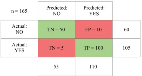
36 Example of a binary confusion matrix . . . 51

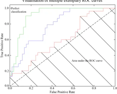
37 Example of a ROC curve . . . 52

41 Visualisation of Intermediate Data Creation . . . 57

42 Visualisation of Intermediate Data Classification . . . 58

43 Samples from CIFAR-10 (from left to right, top to bottom): airplane, auto-mobile, bird, cat, deer, dog, frog, horse, ship, truck . . . 60

44 10 classes from CIFAR-100, like apples, aquarium fish, baby, bed, snake, beetle, bicycle, bottles. . . 62

(19)

45 10 sample classes from ILSVRC-2012 . . . 64

46 Visualisation of First Neural Network Architecture (CNN-1) . . . 69

47 Visualisation of Second Neural Network Architecture (CNN-2) . . . 70

48 Visualisation of SimpleNet Architecture . . . 71

49 Visualisation of VGG-19 Architecture. . . 72

410 Raw example Picture of Class Car . . . 73

411 Normalised Example Picture of Class Car . . . 74

412 MLP-1 Visualisation for CIFAR-10. . . 76

51 Learning Curve of MLP-0 on CNN-1 Intermediate Data for 10 Iterations with Learning Rate 0.0001 . . . 86

A1 Example of deformation . . . 125

A2 Example of occlusion . . . 126

A3 Example of viewpoint variation . . . 126

A4 Example of scale variation . . . 127

A5 Example of background clutter . . . 127

A6 Example of intra class variation . . . 128

A7 Visualisation of general architecture of CNN. . . 129

A8 Normalised images from CIFAR-10 . . . 130

A9 Sample images from CIFAR-100 . . . 131

A19 Sample images from ILSVRC-2012 . . . 143

(20)

A24 CNN1 Accuracy Graph on CIFAR-10 . . . 148

A25 CNN1 Loss Graph on CIFAR-10 . . . 148

A28 SimpleNet Accuracy Graph on CIFAR-10 . . . 149

A29 SimpleNet Loss Graph on CIFAR-10 . . . 149

A34 SimpleNet Accuracy Graph on CIFAR-100 . . . 157

A35 SimpleNet Loss Graph on CIFAR-100 . . . 157

A36 Accuracy Curve of MLP 0 on CNN1 for 10 epochs with a learning rate of 0.0001. . . 158

A37 Loss Curve of MLP 0 on CNN1 for 10 epochs with a learning rate of 0.0001 158 A38 Accuracy Curve of MLP 0 on CNN1 for 20 epochs with a learning rate of 0.0001. . . 158

A41 Loss Curve of MLP 0 on CNN1 for 50 epochs with a learning rate of 0.0001 159 A42 Accuracy Curve of MLP 0 on CNN1 for 10 epochs with a learning rate of 0.001 . . . 160

(21)

A55 Loss Curve of MLP 1 on CNN1 for 50 epochs with a learning rate of 0.001 164

A62 Accuracy Curve of MLP 2 on CNN1 for 50 epochs with a learning rate of 0.001 . . . 166

(22)

41 CIFAR-10 Benchmarks . . . 61

42 CIFAR-100 Benchmarks. . . 61

43 ILSVRC 2012 Benchmarks . . . 64

51 CIFAR-10 Intermediate Dataset Results, trained on MacBook Pro . . . 80

52 CIFAR-100 intermediate dataset results . . . 82

53 ILSVRC-2012 Intermediate Dataset Results for 100 Classes . . . 84

54 CIFAR-100 MLP Classification Results on CNN-1 Intermediate Data . . . 87

55 CIFAR-100 MLP Classification Results on CNN-2 Intermediate Data . . . 87

56 CIFAR-100 MLP Classification Results on SimpleNet Intermediate Data . 88

57 CIFAR-100 MLP Classification Results on VGG-19 Intermediate Data . . 88

58 CIFAR-10 Final Classification Results on CNN-1 Intermediate Data . . . 91

510 CIFAR-10 Final Classification Results on SimpleNet Intermediate Data . 92

511 CIFAR-10 Final Classification Results on VGG-19 Intermediate Data . . . 92

514 CIFAR-100 Final Classification Results on SimpleNet Intermediate Data . 96

515 CIFAR-100 Final Classification Results on VGG-19 Intermediate Data . . 96

516 ILSVRC-2012 Final Classification Results on Inception V3 Intermediate Data . . . 100

517 ILSVRC-2012 Final Classification Results on Xception Intermediate Data 100

518 ILSVRC-2012 Final Classification Results on Inception ResNet V2 Interme-diate Data . . . 100

A1 CIFAR-10 final classification results on CNN-1 intermediate data . . . 150

A2 CIFAR-10 final classification results on CNN-2 intermediate data . . . 150

A3 CIFAR-10 final classification results on SimpleNet intermediate data . . . 150

A4 CIFAR-10 final classification results on VGG-19 intermediate data . . . . 151

A5 Pairwise p-values of performance on validation set with performance on test and validation set displayed on the diagonal for MLP-1, MLP-2, MLP-3 on CNN-1 intermediate data from CIFAR-10 with di↵erent learning rates (LR) . . . 152

(23)

A7 Pairwise p-values of performance on validation set with performance on test and validation set displayed on the diagonal for 1, 2, MLP-3 on SimpleNet intermediate data from CIFAR-10 with di↵erent learning rates (LR) . . . 153

A8 Pairwise p-values of performance on validation set with performance on test and validation set displayed on the diagonal for MLP-1, MLP-2, MLP-3 on VGG-19 intermediate data from CIFAR-10 with di↵erent learning rates (LR) . . . 153

A9 Pairwise p-values of performance on validation set with performance on test and validation set displayed on the diagonal for di↵erent classification algorithms on CNN-1 intermediate data from CIFAR-10 . . . 154

A11 Pairwise p-values of performance on validation set with performance on test and validation set displayed on the diagonal for di↵erent classification algorithms on SimpleNet intermediate data from CIFAR-10 . . . 154

A12 Pairwise p-values of performance on validation set with performance on test and validation set displayed on the diagonal for di↵erent classification algorithms on VGG-19 intermediate data from CIFAR-10 . . . 155

A13 CIFAR-100 final classification results on CNN-1 intermediate data . . . . 167

A14 CIFAR-100 final classification results on CNN-2 intermediate data . . . . 167

A15 CIFAR-100 final classification results on SimpleNet intermediate data . . 168

A16 CIFAR-100 final classification results on VGG-19 intermediate data . . . 168

A19 Pairwise p-values of performance on validation set with performance on test and validation set displayed on the diagonal for MLP-1, MLP-2, MLP-3 on SimpleNet intermediate data from CIFAR-100 with di↵erent learning rates (LR) . . . 170

(24)

A20 Pairwise p-values of performance on validation set with performance on test and validation set displayed on the diagonal for MLP-1, MLP-2, MLP-3 on VGG-19 from CIFAR-100 intermediate data with di↵erent learning rates (LR) . . . 170

A23 Pairwise p-values of performance on validation set with performance on test and validation set displayed on the diagonal for di↵erent classification algorithms on SimpleNet intermediate data from CIFAR-100 . . . 172

A24 Pairwise p-values of performance on validation set with performance on test and validation set displayed on the diagonal for di↵erent classification algorithms on VGG-19 intermediate data from CIFAR-100. . . 172

A25 ILSVRC-2012 final classification results on Inception ResNet V2 interme-diate data . . . 173

A26 ILSVRC-2012 final classification results on Inception V3 intermediate data 173

A27 ILSVRC-2012 final classification results on Xception intermediate data . 173

A28 Pairwise p-values of performance on validation set with performance on test and validation set displayed on the diagonal for di↵erent classification algorithms on Inception ResNet V2 intermediate data from ILSVRC-2012 with 100 classes . . . 175

A29 Pairwise p-values of performance on validation set with performance on test and validation set displayed on the diagonal for di↵erent classification algorithms on Inception V3 intermediate data from ILSVRC-2012 with 100 classes. . . 175

A30 Pairwise p-values of performance on validation set with performance on test and validation set displayed on the diagonal for di↵erent classification algorithms on Xception intermediate data from ILSVRC-2012 with 100 classes. . . 175

(25)

(26)

1 Routing Algorithm from [79] . . . 26

2 Splitting Attribute Selection . . . 32

3 ID3 algorithm from [61], p. 18 . . . 32

4 General Boosting Procedure . . . 35

5 AdaBoost algorithm from [101], p. 801 f. . . 37

(27)

(28)

HDF5 Hierarchical Data Format 5 (HDF5) is a data storage format. It is supported by many programming languages and freely usable. JFT-300M JFT-300M is a dataset of more than 375 million images with noisy

labels. It was developed by Google. The dataset is not publicly acce-sible.

LeNet-5 LeNet-5 is one of the first ever designed convolutional neural net-work. It was created by LeCun et al. in 1998 to automate the process of handwriting detection of digits in checks.

MNIST database The Modified National Institute of Standards and Technology (MNIST) database is a database of handwritten digits. It found its way into multiple research and practical applications, mainly in the field of computer vision.

Python Pickle Python Pickle is a Python-specific data format that is used to serialise data. It can be used to serialise any kind of Python object. Pickle is a binary serialisation format and, therefore, only readable by machines. WordNet WordNet is a hierarchical lexical database that structures words into synsets. A synset is a set of synonyms for a given concept. WordNet is designed for the English language.

(29)

(30)

ADB Adaptive Boosting (AdaBoost) Classifier. ANN Artificial Neural Network.

AUC Area under the curve.

CART Classification and Regression Trees. CNN Convolutional Neural Network.

DT Decision Tree.

ELU Exponential Linear Unit.

FN False Negatives.

FP False Positives.

FPR False Positives Rate.

GAN Generative Adversarial Networks. GBC Gradient Boosting Classifier. GRU Gated Recurrent Unit. ID3 Iterative Dichotomiser 3.

ILSVRC-YYYY ImageNet Large Scale Visual Recognition Competition YYYY.

KNN K-Nearest Neighbours.

LR Logistic Regression.

LSTM Long Short Term Memory Networks.

MECE Mutually Exclusive Collectively Exhaustive. MLP Multi Layer Perceptron.

(31)

OCR Optical Character Recognition. ReLU Rectified Linear Unit.

ResNet Residual Network.

RFE Random Forests Classifier/Estimator. RGB Red Green Blue.

RNN Recurrent Neural Networks. ROC Receiver Operating Characteristic. SVM Support Vector Machine.

TN True Negatives. TP True Positives. TPR True Positives Rate. Xception eXtreme Inception.

(32)

Chapter

1

Introduction

1.1 Background Information

Computer vision is a sub-field of artificial intelligence and computer science that enables computers to develop a visual perception of real-world entities. Computer vision is about the automatic extraction, analysis, and understanding of information from imagery data. The field of computer vision can be divided into multiple sub-areas that each focus on specific information of the image data, summarised in figure11:

1. Classification: Image classification is about the assignment of a label from a predefined fixed set of categories to an input image. It can be seen as the core of most computer vision tasks because all of the subsequently introduced sub-fields rely on image classification.

2. Localisation: Object localisation enhances the scope of image classification to adding information about the position of the identified object. Thus, additionally to identifying the object in question, the algorithm needs to find the object in the picture and determine its position. This is often done with bounding boxes, where the object is surrounded by a rectangular box indicating its position in the image. Object localisation consists of a classification and a regression problem. 3. Detection: Object detection enlarges the scope of object localisation in the sense

that multiple objects from di↵erent classes can be identified and localised in an image. Given a fixed set of categories and an input image, the task of an object detection algorithm is to return the position and the type of every identified occurrence of one of the classes. Object Detection itself does not only consist

(33)

Figure 11: Summary of Di↵erent Computer Vision Tasks from [91]

of a regression a classification problem because the number of outputs of the algorithm is variable and not known beforehand.1

4. Semantic Segmentation: Semantic segmentation is a special case of image clas-sification, where each pixel of an image is assigned to a specific category from a predefined set of categories. If an image contains multiple instances of the same base class, they are associated with the same category in semantic segmentation because the algorithm does not distinguish between instances of the same class. 5. Instance Segmentation: Instance segmentation is a special case of semantic

seg-mentation where multiple instances of the same class are classified into di↵erent categories. Given a picture of two dogs in front of a random background and the input classes ”dog” and ”background”, the previously described semantic segmentation would classify each pixel of the dogs as category ”dog” and each pixel from the background as ”background”. Instance segmentation, on the other hand, would classify the two objects from the class dog as two di↵erent categories.

The concepts introduced in this thesis are applied to the task of image classification, but they can be integrated into the classification part of the other computer vision sub-areas.

Computer vision has gained traction since the breakthrough of artificial neural net-works (ANN), which was fostered by the increases in available computational power and training data. But it was only in 2012 when a research team consisting of Alex Krizhevsky, Ilya Sutskever and Geo↵rey Hinton from the University of Toronto con-structed AlexNet [51] for the ImageNet Large Scale Visual Recognition Challenge

1_{more about object detection and how to resolve the problem of object detection can be read}

(34)

(ILSVRC) in 20122_{, that a convolutional neural network (CNN) architecture}

outper-formed traditional approaches in the classification and localisation tasks. This initiated the hype in deep learning for computer vision in the subsequent years [75] [53]3_{. After}

that, CNN architectures were improved in many ways, found their way into multiple fields of research and were successfully applied in the industry. Nonetheless, the same Geo↵rey Hinton that helped CNNs to their success is one of their greatest critics. He came up with the idea of capsule networks with a team of researchers from Google Brain [27], which take a di↵erent approach and give promising results, especially for the case of little training data and strong variations within training and test data [79]. Although these networks are conceptually fundamentally di↵erent to CNNs, they still make use of convolutional layers and fully-connected layers4.

1.2 Structure of the Thesis

Although a general introduction to multi-layer perceptrons (MLPs) is given in sec-tion 3.6, the thesis assumes a general knowledge of important concepts related to ANNs, including the concepts of batch learning, gradient descent, activation functions and the notions of overfitting and generalisation. Further reading on these topics can be done in [26], [32]. Chapter 2 explains convolutional neural networks, the most relevant innovations, and state-of-the-art architectures. Chapter 3introduces di↵erent classification algorithms that are commonly used in machine learning. Fur-thermore, di↵erent evaluation methods for model performance on classification tasks are presented. Afterwards, chapter 4outlines the experimental setup of the thesis used to test the research question proposed above, including the datasets, the network architectures, the chosen classification algorithms, the software architecture to test the research question and the evaluation metrics applied. Lastly, chapter5provides an evaluation of the experimental results. Along with presenting the intermediate datasets created from the high-level image features, the chapter describes the final results, makes a comparison and a final evaluation.

1.3 Purpose of the Thesis

Image Recognition is arguably one of the most active parts of research within machine learning. Before the dominance of neural networks in computer vision research, "in the traditional model of pattern recognition, a hand-designed feature extractor gathers relevant information from the input and eliminates irrelevant variabilities. A trainable classifier then categorises the resulting feature vectors into classes."([105], p.5) In this traditional model, any classification algorithm is used to distinguish the classes

2_{referred to as ILSVRC-2012}

3_{they used the team name ”SuperVision”}

(35)

based on the hand-designed image features. The emergence of convolutional neural networks in computer vision meant a shift from hand-designed feature extractors to automatically generated feature extractors trained with backpropagation.

As chapter 2 shows, there have been many developments of CNN architectures re-cently that substantially change the model architectures. But chapter2also shows that all of these advances have been made in the earlier layers of the neural network, mean-ing everythmean-ing up to the fully-connected layers. Little research has been devoted to the proficiency of the fully-connected layers. Fully-connected multi-layer perceptrons (MLP) seem to be the design choice for all network architectures with little research or modifications done to these layers. But as the no-free-lunch theorem from chapter3

shows, no classifier can be said to be superior to all other classifiers. Therefore, follow-ing the idea of the traditional model of pattern recognition where any classification algorithm was used, the evolved research question for this thesis is:

Research Question ”Can classification model performance in computer vision be im-proved by using di↵erent classification algorithms on high-level image features?”

Both convolutional and fully-connected layers of a neural network learn their weights during training with the weights being backpropagated from the output through the fully-connected-layers back to the convolutional layers. Due to this nature of the learning process, multi-layer perceptrons are a natural choice for convolutional neural networks. Convolutional neural network features can only be learned through a back-propagated error that usually comes from a multi-layer perceptron or directly from the output. Therefore, the focus of this thesis is not directly on replacing the fully-connected layers in the learning process, but rather enhancing the learning process to a two-step procedure:

1. Regular CNN Training Process: Train a given CNN architecture, including fully-connected layers to make convolutional layers learn image features from image inputs

2. Enhancement of the Training Process: Replace the fully-connected layers with a di↵erent classification algorithm and train the algorithm based on the high-level image features produced from the convolutional layers in the first step

This research question is tested in multiple settings on multiple datasets to investigate further under which conditions certain classification algorithms potentially perform better. The datasets benchmarked in this thesis are CIFAR-10, CIFAR-100 and a subset of ILSVRC-2012.

(36)

Chapter

2

Artificial Neural Networks for Computer

Vision

In the late 19th _{century, the Spanish neuroscientist Santiago Ramon y Cajal}

discov-ered that the human nervous system consists of many independent nerve cells that are connected through nerve synapses that transfer nerve impulses between the cells. His works contributed significantly to the understanding of the human brain and the human thought process, which is the foundation for human intelligence. Neurosci-entists and computer sciNeurosci-entists, such as McCulloch and Pitts (1943) [62], Rosenblatt (1958) [73], Paul Werbos (1974) [104], Rumelhart, Hinton, Williams (1986) [74] and others, used this idea of how the human brain works to develop, train and improve artificial neural networks. Following a period of disrepute, data became more easily accessible through the internet and computational means increased following Moore’s Law1_{, ANNs gained popularity again and found their way into the industry. The}

break-through of ANNs led to an increase in research in the area and the development of advanced network architectures for specific domains, such as recurrent neural net-works (RNNs) and their variations long short-term memory netnet-works (LSTM) [37] and gated recurrent unit networks (GRU) [13], generative adversarial neural networks (GAN) [25] and others.

Although the visual perception of objects is an easy task for most human beings, it was traditionally not a task that computers were particularly good at. The 1980s brought some theoretical advances on custom tailored problem domains, but they were not widely applicable in practice. In the early 20th_{century, the idea of developing features}

(37)

that are invariant to changes emerged. The idea is to identify critical features (building blocks) of an object and match these features to similar objects rather than pattern matching the entire object. This idea of leveraging object features along with the increasing popularity of ANNs gave rise to the breakthrough of convolutional neural networks.

2.1 How are Digital Images Represented

Before the introduction of convolutional neural networks, a common understanding of digital images is necessary.

An image is a two-dimensional function f (x,y) that describes the color f at the spatial coordinates (x,y). A digital image is one where x, y, and f are finite, meaning the spatial coordinates are covered by a predefined number of elements, called pixels. The computational representation of a digital image is a three-dimensional array with the dimensions width w, height h and depth d: I 2 Rw⇥h⇥d_{. Whereas width w and height}

h determine the shape of the pixel grid of an image, the depth determines the colour

of a given pixel and is described by an array of length d. Common representations of images are grey-scale (d = 1) and RGB (d = 3). The depth is also referred to as the number of channels ([99], p. 3) but the author of this thesis chose to use the notion of depth to describe input and output channels.

Features of an image are any patterns of pixels that have unique shapes. Low-level features are simple shapes, e.g., lines and edges of di↵erent intensities. Higher-level features are combinations of multiple layers of lower-level features. Higher-level level features are more complex patterns and a combination of multiple lower-level features, e.g., a nose made up of multiple lower-level edges. The detection of features within an image is done with image filters. Each filter is responsible for detecting the existence of one feature. For more, see section2.3.1.

2.2 Challenges in Computer Vision

Perturbation of imagery data can occur in any of the three dimensions. An object in question can be shifted, scaled or distorted in the grid and change its colour values while still belonging to the same category of images. Further variations regard the object itself and within its context, such as

• Deformation: The real-world object can take on di↵erent shapes and poses and be deformed in many ways.

(38)

• Occlusion: The real-world object could be occluded, e.g., the real world entity hides behind another object with just a part of it visible in the image.

• Viewpoint Variation: The image data can capture a real-world entity from dif-ferent perspectives.

• Scale Variation: Apart from the scale variation within an image representation, real-world entities can also vary in size while still belonging to the same category. • Background Clutter: The object and its background are composed of similar

colours or structures and thus make it hard to di↵erentiate between them. • Intra-class Variation: Chosen classes usually represent concept from the real

world. These concepts can be rather broad with many intra-class variations. For example, the concept of a dog can be represented by di↵erent breeds while still belonging to the class dog.

For a visual understanding of these challenges, see AppendixA.1.1.

An ideal computer vision algorithm is robust to all these intra-category variations within the images, while perceiving inter-category di↵erences.

2.3 Convolutional Neural Networks

The neurobiologists David Hubel and Torsten Wiesel analysed the visual processing mechanisms in mammals in 1959, using cats as a reference to understand the human visual system. They attached electrodes to the back of the brains of cats to examine which visual stimuli makes the neurons in the primary visual cortex of a cat brain respond. They found out in their research that visual processing begins with simple, low-level structures of the world, such as edges and their orientations, which are then aggregated to more complex, high-level concepts in the visual processing pathway. Transferring this idea of the visual system to humans, one can conclude that the hu-man brain builds up the perception of an object by aggregating multiple low-level image features and successively combining these building blocks to a larger high-level representation.

Convolutional neural networks adapt this principle from nature in that they aim to automatically detect high- and low-level features within the network during the training process. CNNs combine the architectural ideas of local receptive fields from section2.3.1, shared weights (weight replication) from section2.3.1, and spatial sub-sampling from section2.3.3. ([105], p.6)

(39)

The ability of multi-layer networks trained with gradient descent to learn complex, high-dimensional, non-linear mappings from large collections of examples makes them obvious candidates for image recognition tasks. LeCun et al. (1998) ([105], p.5)

Not only does this notion of learning more accurately imitate the human brain because CNNs automatically detect 2-dimensional local structures within images without prior manual definition. CNN structures are also computationally more efficient in compar-ison to their fully-connected counterparts because the convolutional network layers require fewer weights. Thus, the model has to learn fewer parameters during the training process.

The first published CNN, LeNet-5, was developed by LeCun et al. (1998) and was applied in alphanumeric character recognition to read ”several million checks per day” ([105], p.1) automatically in 1998.

Figure 21: LeNet-5 Architecture from LeCun et al. (1998)

After their introduction, CNNs remained at the sidelines of research until AlexNet won the ILSVRC-2012 challenge in the classification and localisation task by a great margin compared to the other approaches. ILSVRC is the most famous computer vision challenge based on the ImageNet database, as introduced in section4.3.3. For the classification task, AlexNet reached a top-5 error of 15.32 %, whereas the next best model architecture reached 26.17 %. AlexNet [51] is an 8-layer neural network that strongly resembles LeNet-5 from figure21in its architecture. After this success, CNNs became state-of-the-art in computer vision with more and more innovative additions to the networks outperforming earlier models. The next decisive changes to the network architecture were introduced in ILSVRC-2014, with GoogLeNet from Szegedy et al. (2014) and VGG from Simonyan and Zisserman (2015) reaching a top-5 error of 6.67 % and 7.32 % respectively ([95], p. 9) [54]. The main contribution of VGG was to use relatively small convolutional filters combined with deeper neural networks (16-19 layers) [86]. GoogLeNet is a 22-layer network without fully-connected layers at its end. Its main contribution to subsequent model architectures is the inception module (see section2.3.7). Apart from computational limitations, a roadblock to even deeper

(40)

neural network architectures was the fact that deeper networks empirically produced worse results on training and test data [31]. They should, in theory, be at least as good as their shallower counterparts. The ResNet-152 architecture from He et al. (2015) won the ILSVRC-2015 challenge with a top-5 error of 3.57 %. With a depth of 152 layers, it is the first model to beat human performance. The solution to training deeper networks are residual blocks (see section2.3.8), giving the name to ResNet. [31] [54]

The following subsections will explain the introduced concepts in more detail. The following sections show the key areas of research and improvements to CNNs from the past few years.

2.3.1 Convolutional Layers

A convolutional layer creates an n-dimensional output representation (depth n) of given input data (e.g., digital image data, see section2.1), where each dimension is created with respect to one image filter. A convolutional layer consists of at least one, though usually multiple, di↵erent image filters ([105_{], p. 6), thus n 2 N}₁.

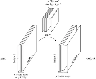
Figure22visualises the concept of one convolutional layer. The convolutional layer consists of n filters. These n filters are applied on the input image. In this case, the input image consists of three feature maps, as would be the case for an RGB image. Through the application of these n filters, an output image with n feature maps is created. This output image will then be the input for the next convolutional layer.

Figure 22: Application of convolutional layer with n image filters of size kw⇥ kh⇥ 3 with stride s = 1 on input data with size widthw ⇥ height h and an input depth of 3 [99]

(41)

The following subsections introduce the concept of image filters, how they can be learned and common model choices.

Image Filters

The following chapter introduces the concept of image filters for two-dimensional im-ages. These two-dimensional images can still have three-dimensional representations in digital formats, e.g., if the color is represented in RGB format. Nonetheless, the concepts introduced can easily be enhanced to inputs with more spatial dimensions. This thesis only handles two-dimensional images.

An image filter (also called filter kernel) is a tensor F 2 Rkw⇥kh⇥Id, where k

w, kh 2 N₁ determine the filter’s width and height respectively, and Id corresponds to the depth of the input image to the convolutional layer. The output image I0 _{is produced}

through a convolution of the input image I 2 Rw⇥h⇥d _{with the image filter. Basically,}

the Hadamard product is applied to the image filter and a local input field, called receptive field, of size kw⇥ kh⇥ Id with center (x,y). Each entry, e.g., pixel, in the grid of the output image I0_{(x,y) is thus calculated as a sum of these point-wise multiplied}

tensors. ([99], p. 3)

The formula for a given output entry can be found in equation2.1([99], p. 3).

I0(x,y) = b + kw 2 X ix=1 kw2 kh 2 X iy=1 kh2 Id X ic=1 I(x + i_x, y + i_y, i_c) · F(ix, iy, ic)

for x 2 {1,··· ,Iw} and y 2 {1,··· ,Ih}, where b 2 R denotes the bias

(2.1)

Due to the aggregation from the summing operations, the depth of the output from a single image filter is always 1.

(42)

Figure 23: Visualisation of application of a linear k ⇥ k ⇥ 1 image filter on receptive field in input [99]

Formula2.1states the calculation of the output pixel at I0_{(x,y) for a given receptive}

field with center I(x,y). This operation is applied for all pixels x 2 {1,··· ,Iw}, y 2 {1,··· ,Ih} and for all n image filters to create the full output image I 2 Rw0⇥h0⇥d0. In this case, the image filter operation can be thought of as sliding over the input image from the top left to the bottom right corner, shifting the center of the receptive field by 1 unit and performing the convolutional operation to produce the output data. Every output position can be regarded as a score of how well the given receptive field responded to the image filter. The higher the score of the output position, the more likely it is, that the receptive field in the input data was representing a structure formalised by the image filter. In the end, the output data will have a score at each position, indicating the likelihood that the image filter representing a given feature is present at that position in the input data. This also makes CNNs more robust to distortions and shifts of the object within an input image, because a distortion or shift would eventually lead to a distorted or shifted value in the output image. It follows that the feature would still be detected while its exact position is irrelevant.

But the question remains of how a receptive field greater than 1 can be produced at the image boundaries. In other words: What is the receptive field when the centre lies at the border of the image, and the receptive field would thus partially fall out of the boundaries of the input data? The two most common approaches to border handling are ([28], p. 3):

• Eliminate the border-dependent pixels by cropping the output image to perform convolution on the inner pixels only where possible or

(43)

• Pad the input image to account for the missing input pixels.

The first approach implies a diminishing output size of kw 1 and kh 1 for the width and height respectively of the convolutional layer. The second approach requires a padding technique. Common techniques are ”replicate”, ”reflect”, ”wrap” and ”con-stant” (e.g., zero-padding) (for more, see [28]).

As described above, performing this convolution leads to an overlap between the re-ceptive fields of contiguous input positions. One hyper-parameter of the convolutional layer is the stride s 2 N1. The stride determines by how many contiguous input

posi-tions the receptive field should be moved when creating the image output. The case described above uses a stride of 1, meaning no input position is skipped. If the stride is chosen to be bigger than 1, the e↵ective output image gets reduced in size. Apart from the stride, the output image size is only determined by the border handling procedure for uneven filter sizes. Usually, the stride and border handling are chosen such as to preserve the image size. The filter width and height are commonly set to be uneven. Each image filter performs k_w⇥ kh⇥ Id multiplications at each position of the input. Hence, over the full image, each filter performs I0

w· Ih0 · kw· kh· Id multiplications. For

knimage filters, each convolutional layer then performs the following number of mul-tiplications2_:

k_n· Iw0 · Ih0 · kw· kh· Id (2.2)

Convolutional Layer Training

During training, the convolutional layers learn to construct the image filters. The weights of the image filters are the parameters of the learning process that are adapted to the training data ([99], p. 5). Convolutional layers leverage the concept of shared weights for the learning process, introduced by Waibel et al. (1989). Since the identical image filter is repetitively applied over the positions in the input image, this is like connecting a given position from the image filter to each input position with the same weight. The sizes of the receptive fields determines the number of necessary weights. Hence, k_w· kh+ 1 (bias) parameters need to be learned per image filter.

Because of the concept of shared weights, every convolutional layer can be formulated as an MLP, with the drawbacks of then having more parameters to train. Nonetheless, this shows that a convolutional layer can be trained using gradient descent [60]. But for the case of shared weights as in CNNs, the training algorithm is changed to account 2_{Assuming that the initial image dimensions are preserved, e.g., a stride of 1 and padding for border}

(44)

for ”the average of all corresponding [...] weight changes” ([100], p. 331) with respect to the training data.

Convolutional Layer Hyper-Parameters The hyper-parameters to tune are ([99], p.5)

• the number of image filters n 2 N1

• the image filter width and height k_w, k_h2 N1

• the activation function after the convolution • the stride s 2 N1

• the border handling function

Typical choices for n are values of an exponential function to the base 2 (numbers from the binary series), e.g., n 2 {25_{, 2}6_{, 2}7_{}, up to 2}11_{. The kernel width k}

wand height khare usually chosen to be equal and uneven. thus kw= kh= k 2 {1,3,5,7,11}. The activation function is usually a rectified linear unit (ReLU) activation or other derived versions, such as ELU. The stride is usually set to s = 1 ([99], p. 5) and border handling is usually done through constant padding with 0s.

As outlined before, the inventors of VGG, Simonyan and Zisserman (2015), discovered that shallower but deeper networks are advantageous compared to their flatter but wider counterparts. The intuition behind using smaller filters combined with deeper networks is that the deeper networks can have the same e↵ective receptive field as the wider network, but also increase the non-linearity and reduce the model parameters. The winners of ILSVRC-2013, Zeiler and Fergus, use 96 di_{↵erent 7 ⇥ 7 convolutional} filters in the first hidden layer of their network ([111]: p. 6). Assuming a stride of 13, using three layers of 3 ⇥ 3 convolutional filters has the same e↵ective receptive field as a 7 ⇥ 7 filter. Apart from the increased non-linearity through a deeper network, this separation reduces the model parameters in the convolutional layers. In this example, the parameters per channel reduce from 72_{for one layer with a receptive field of 7 ⇥ 7}

to 3 · 32_{for three layers with receptive fields of 3 ⇥ 3. [}₈₆_]

2.3.2 Depthwise Separable Convolutions

Convolutional layers are computationally expensive because they perform many mul-tiplications, as shown in equation2.2. This number of multiplications can be a bottle-neck when training large convolutional neural networks.

(45)

Depthwise separable convolution, as introduced by Chollet (2016) [12], breaks down the procedure of applying image filters from section2.3.1into two steps:

1. Depthwise Convolution: While regular convolution applies the image filter F on all channels in the input depth I_d, depth-wise convolution applies I_dimage filters with a depth of 1: k_w⇥ kh⇥ 1. These image filters of depth 1 are applied on all input channels, thus Id times. The resulting cubicle is of output size Iw0 ⇥ Ih0⇥ Id4. This produces I0

w· Ih0 · kw· kh· Id multiplications.

2. Pointwise Convolution: The input to the pointwise convolution is the output from the depth-wise convolution and thus of size I0

w⇥ Ih0⇥ Id. On this input, 1 ⇥ 1 convolutions are performed with a filter depth of I_d according to the number of input layers. These 1 ⇥ 1 convolutions inevitably preserve the image width and height. According to the number of desired output filters, these 1⇥1 convolutions are performed k_ntimes. Therefore the output image I0 _{will be of size I}0

w⇥ Ih0⇥ kn. In total, that leads to Id· Iw0 · Ih0 · knmultiplications per convolutional layer.

The total number of multiplications thus amounts to the following number of calcula-tions:

I_w0 · I_h0· kw· kh· Id+ Id· Iw0 · Ih0 · kn= Iw0 · Ih0 · Id· (kw· kh+ kn) (2.3)

The ratio between the original convolution from equation 2.2 and the depth-wise separable convolutions from equation2.3for the identical target image dimensions I0

is then I_w0 · I_h0 · Id· (kw· kh+ kn) kn· Iw0 · I_h0· kw· kh· Id = k_w· kh+ kn kw· kh· kn = 1 kw· kh + 1 kn (2.4)

This ratio is smaller than or equal to 1 for all cases where k_n 2 ^ kw· kh 2 and thus depth-wise convolutions are usually more efficient than regular convolutional layers.

The ratio for the number of parameters between the regular convolution and the depth-wise separable convolution is equal to the ratio of the multiplications in equation2.4. Thus, this is also usually reduced.

Apart from the eXtreme Inception (Xception) neural network architecture from Chol-let (2016)[12], the idea of depth-wise separable convolutions is used in many other model architectures, such as MobileNet [39], a neural network designed to run on

4_{assuming that initial dimensions are preserved during the convolution, the output size is I}

(46)

the limited hardware capabilities of end-user smartphones, in a proposed neural ma-chine translation architecture [45] and a multi-purpose model designed by Kaiser et al. (2017), used for translation, image classification, speech recognition and parsing [46].

2.3.3 Pooling Layers

Pooling Layers

• make networks robust to translational variance,

• make networks robust to minor local changes and

• reduce the size of the data.

A pooling operation makes a summary of a receptive field p_w⇥ ph, pw, ph2 N1, of the

input data. It is responsible for the routing of information through the network by deciding which information to pass on to the next layer. Equivalently to the image filter in convolutional layers, the pooling operation is performed over the positions of the input image with a predefined stride s 2 N1. Usually, the stride is chosen to be

larger than 1, such that the pooling layer reduces the size of the input data by a factor of

s2. The pooling window defined by p_wand p_h can be any subset of the input image. If

pwand phare equal, the pooling window preserves the ratio between width and height from the input image. Thus, they are typically chosen to be equal and between 2 and 5, depending on the input image size and other factors (see also [51], [86], [95], [31]). As the pooling operation only summarises the input data, which is usually passed through an activation function before, it is not common to apply an activation function after this layer. If padding is applied at the borders, Max-Pooling uses 1 values at the overlapping areas such that these entries cannot possibly be the maximum values for the max pooling operation.

Typical pooling functions are Max-Pooling, Average/Mean-Pooling, L2-Pooling, Stochastic-Pooling, Spatial Pyramid Pooling and Generalising Pooling Functions (for more, see [110], [7], [8], [57]).

The pooling function is often criticised due to its inevitable information loss. By sub-sampling the data and making it invariant to small perturbations, it loses the precise spatial relation between higher-level features (see also section2.3.9).

(47)

2.3.4 Fully-Connected Layers

Fully-connected layers are layers with neurons that have full connections to all out-puts from the previous layer. While the convolutional and pooling layers perform the detection and extraction of features from an image, the fully-connected layer(s) of a convolutional neural network create the final output of the network. Fully-connected layers of a convolutional neural network ”are required to learn non-linear combina-tions of learned features” ([3], p. 2) from the previous layers. Fully-connected layers are simply a multi-layer perceptron classifier, as introduced in3.6.

As described in sections2.3.1and2.3.3, the output from the previous layer is a tensor

I 2 Rw⇥h⇥n_{. Since fully-connected layers have no notion of the location of the input,}

they work with dimensional input data. Therefore, the data is flattened to be a 1-dimensional feature vector. As introduced in section2.3.1, convolutional layers are simply a specific case of regular fully-connected layers. Thus, what is referred to as fully-connected layers in neural networks are technically 1 ⇥ 1-dimensional convolu-tions with a full connection table, meaning there are no shared weights.

The numeric restrictions of the output depend on the problem domain. The output is either continuous for regression problems or a likelihood score for a classification problem with each output value indicating the probability for a given class. The likelihood is usually expressed between 0 and 1, e.g., through the application of a softmax function. The number of output neurons for the final fully-connected layer (output layer) is equivalent to the number of desired output classes. For a classification problem with n classes, the output is usually of length n and bounded between 0 and 1, such that every output neuron reflects the probability of a given class. Alternatively, each output neuron can reflect a binary value that encodes the classification. For this case, log2n output neurons are necessary.

2.3.5 Dropout Layer

Dropout is used to foster generalisation of the learning process and prevent overfit-ting. Hinton et al. [34] introduced the idea of dropout to neural networks. Dropout means randomly deactivating certain neurons with a probability p during each run of the learning process. Neurons are deactivated by setting their output to 0. Dropout forces the network to more robustly learn features with multiple neuron combina-tions without the ability to ground certain assumpcombina-tions on specific neurons (for more see [89]).

A dropout layer is simply a tensor D 2 Rw⇥h⇥d _{of the shape of the input data that}

contains a 0 or a 1 for every position, depending on whether the neuron is activated (1) or not (0). Thus, dropout is calculated as the Hadamard product between this dropout

(48)

tensor and the input data: D in. Every element di in D is independently sampled from a Bernoulli distribution with probability p. Since dropout reduces the number of outputs created from the network, the final output is multiplied with 1

1 p when

dropout is applied to account for the missing neurons.

The dropout probability p is a hyper-parameter of the layer, typically set to 0.5. Fur-thermore, layers closer to the output tend to have higher dropout probabilities than layers closer to the input.

Dropout is only done during the training phase and not at inference time.

2.3.6 Batch Normalisation Layers

Batch normalisation is a means for more efficient deep network training by reducing internal covariate shift. Internal covariate shift refers to the phenomenon that the out-puts of the nodes of di↵erent layers of a neural network follow di↵erent distributions ([85], p. 228). Internal covariate shift is mainly caused by layers closer to the output learning better with respect to the error than layers closer to the input.

Batch normalisation enables a more stable gradient propagation in a neural network, especially for deep neural networks. It can also lead to speed improvements in the learning process ([15], p.1), the possibility to use ”higher learning rates without the risk of divergence and other ill side e↵ects” ([80], p.59). It further reduces the risks associated with saturating nonlinearities (e.g., softmax) ([43], p.2) and can improve parameter initialisation ([43], p.1).

The method from Io↵e and Szegedy (2015) performs a point-wise normalisation over the mini-batches with input x = (X(1)_,_{··· ,X}(d)_{). The formula is as follows:}

ˆx(k)=qx(k) ¯x(k)

s0⇣x(k)⌘2+ "

(2.5)

with sample mean ¯x(k)₌ 1

m P_m

i=1x

(k)

i and sample variance s0 ⇣

x(k)⌘2=_m1Pm i=1

⇣

x(k)_i ¯x(k)⌘

and mini-batch sample size m 2 N1and constant " > 0 2 R.

This is an adjusted calculation of z-score normalisation over the mini batch by sub-tracting the sample mean and dividing by an adjusted sample standard deviation. The standard deviation is adjusted by adding a small constant " to account for the case of no variance in the data (division by zero).

(49)

in the training process.

y(k)= (k)· ˆx(k)+ (k) (2.6)

These parameters allow for the model to adjust the normalisation that was done be-fore. For example, they enable the normalisation layer to become an identity layer by reverting the standardisation by the sample variance for and sample mean for , thus simply passing the input data through.

Adjusted forms of normalisation exist (for more, see [102]), though batch normalisation is the most common one.

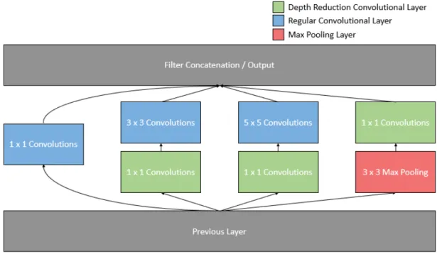
2.3.7 Inception Modules

An inception module5, introduced by Szegedy et al. (2014) [95] follows the idea of a network within a network, initially introduced by [58]. An inception block is a summary of multiple contained layers. The idea is to design a good local network topology that can then be combined to a larger network. These sub-network operations are performed in parallel and concatenated depth-wise at the end. Each sub-network consists of convolutional layers or pooling layers.

As in the case for GoogLeNet, the inception module contains convolutional layers with receptive field sizes of 1 ⇥ 1, 3 ⇥ 3, and 5 ⇥ 5 and a 3 ⇥ 3 max pooling operation, see figure24.

Figure 24: Simple Inception Module, modified from Szegedy et al. (2014) [95] 5_{also called inception module, concatenation block, aggregation block}

(50)

The abovedescribed model architecture adds multiple convolutional layers to the net-work and thus requires additional parameters to be learned.

In the following, the input image to the inception module is denoted as Iinp_{, with the} dimensions Iwinp, I_hinpand I_dinp. The input to a given image filter k is denoted as Ikand is equal to Iinp _{when k is performed directly on the input. The set of initial nodes} in the inception block are referred to as inception nodes Kinc_{. The set of added 1 ⇥ 1} convolutions are referred to as reduction nodes Kred_{. The set of all convolutional layers} is represented by K \ K1_{, with k}

w 2 and kh 2. The set of 1 ⇥ 1 convolutions, where

kw = kh = 1, is referred to as K1. All complexity reduction convolutional nets that occur after a pooling layer are referred to as Kaf ter_pool_{. Furthermore, a stride of 1 and} padding at the borders for both convolutional and pooling layers are assumed in this subsection to preserve the image dimension and facilitate the computation. The idea of an inception module works independently of the stride and border handling function chosen as long as the dimensions are identical for the depth-wise concatenation. Given the setup introduced above, each convolutional layer k in the set of all convolu-tional layers Kinc_{performs I}inp

w ·I_hinp·I_dinp·kw·kh·knoperations. For the computationally complex inception module from figure24, the number of computations is shown in equation2.7.

Operations_complex= Iwinp· I_hinp· X k2Kinc

I_dinp· kn· kw· kh (2.7)

For the network structure in figure24, this means Iwinp· I_hinp· I_dinp· (kn1+ 9kn2+ 25kn3) convolutional operations. It can be easily seen how this number gets large quickly and hinders network performance. This problem is amplified by the fact that the layers are concatenated depth-wise. The final depth is I_d0 = I_dinp+ kn1+ kn2+ kn3. Since the pooling layer only preserves the depth of the input image I_dinp, concatenation with the convolutional layers can only increase the depth of the output image I0_{. This e↵ect}

increases network size and complexity, especially over multiple inception modules. The abovedescribed problems can be solved with 1 ⇥ 1 convolutions, which serve ”as dimension reduction modules to remove computational bottlenecks” ([95], p. 2). A 1⇥1 convolution preserves the spatial dimensions of an image but can reduce its depth, if kn< I_dk. The 1⇥1 convolution is applied before the original set of convolutions, except if it is a 1⇥1 convolution itself, thus only on Kinc_\K1_{. It is also applied after the pooling}

(51)

Figure 25: Advanced Inception Module designed to reduce the overall complexity, modified from Szegedy et al. (2014) [95]

The first advantage of this network structure is that the depth of the concatenation node is not necessarily larger than the input depth to the inception module because the pooling from the output layer can be down-sampled to length n. Thus the final depth is: I_d0 = X k2Kinc kn+ X k2Kaf ter_pool kn (2.8)

Despite additional complexity ofP_k_2KredI_winp· I_hinp· I_dinp· k_nmultiplications caused by

the additional convolutional layers, the goal is to reduce the overall complexity by reducing the depth parameter in the subsequent layers from I_dinp to knin the formula above.

The total number of operations is thus

Operations_reduced = Iwinp· I_hinp· 0 BBBB @ X k2Kred I_dinp· kn+ X k2Kinc I_dk· kn· kw· kh 1 CCCC A (2.9)

Operations_complexshould be bigger than Operations_reduced. In the following, it is as-sumed that this condition holds and a simplified formula is derived to verify the