A wearable mechanism to assist the knee during the loading response

(1)

Faculdade De Engenharia Da Universidade Do Porto

A wearable mechanism to assist the

knee during the loading response

Lu´ıs Rodrigues de Castro

Dissertation

MSc in Mechanical Engineering

Supervisor: Dr. Vito Monaco, SSSA (Pisa, Italy)

Co-Supervisor: Prof. M´

ario Vaz, FEUP (Porto, Portugal)

(2)

(3)

Abstract

Exoskeletons are assistive devices that have been evolving in the last years, being mostly applied in the military, rehabilitation and ergonomics fields. In addition, they are also being used to increase the human endurance capabilities, by reducing the muscle fatigue and metabolic rate. The aim of this thesis was, in fact, to study a new design for a wearable and passive mechanism that solves those last aspects. In particular, the mechanism is intended to assist the knee during the loading phase of the human gait cycle. The state of art of such passive assistance is typically based on the use of springs (that store and release energy), while, here, a damping-based device was designed, being the damper mechanism responsible for dissipating energy. Moreover, the spring approach does not allow for an easy individual adaptability, as springs must be replaced. In contrast, the damper solution includes a regulator screw, facilitating customization.

Two different solutions were thought and analyzed: a pneumatic one, and another based on a commercial damper. Only the last was further studied due to its higher potential of success.

Before conceptualizing any device, it was necessary to analyze kinetic and kinematic data of the human gait, available in the literature. This data was used to estimate the required damping coefficient of the system, so it could mimic the human knee joint.

Regarding the pneumatic solution, it was, first, designed as a pneumatic spring (stroke of 100mm and initial pressure of 6.9bar) and, afterwards, a simulation using Simulink was used to test the influence of the flow control valve. The simulation showed that the system provided a similar torque to the one produced by the muscles which support the knee. Although these results were promising, the system was not further investigated, due to possible leaks of air and overweight.

For the other solution, a commercial rotary damper was selected, with 40Nm of max-imum torque and low weight (352g). However, its damping characteristics had to be determined experimentally, as no complete datasheet was available. From the mathemat-ical model obtained (damping coefficient as a negative exponential function of the angular velocity), it was concluded that the damper does not provide a similar torque to the knee one. Nevertheless, it can bring energetic reductions, only evaluated with future additional tests. Moreover, the mechanical components, and relevant electronic components, were selected. A 3D model was built in Solidworks and used to explain the device operation.

(4)

(5)

Acknowledgments

I would like to thank Dr. Vito Monaco not only for giving me the opportunity to work in such a prestige university and interesting project, but also for the enormous support given throughout my work. I also thank prof. M´ario Vaz for his guidance in spite of the distance imposed by the project location. Finally, I have to give my best thanks to my family and girlfriend, D´ebora Pereira, for their constant support, both intellectually and emotionally, throughout the thesis.

(6)

(7)

List of Figures

2.1 A) Anatomical planes description. B) Leg diagram in the rest position (0

deg at all joints) with the positive direction indicated. [6] . . . 3

2.2 Summary of the gait phases, pointing their main features. [40]. . . 5

2.3 Kinematic and Kinetic data at the three different walking speeds. [48] . . . 6

2.4 Knee range of motion for a 70 Kg male subject walking at 1 m/s. . . 7

2.5 Knee range of motion for slow, natural and fast walking speeds. [47] . . . . 8

2.6 Knee torque pattern. [48] . . . 9

2.7 Reaction vectors until pre swing. . . 9

2.8 Torque-angle of the biological knee during walking. Linear regression dur-ing stance and swdur-ing phase. [9] . . . 10

2.9 Top left : Peak Knee Flexion Moment at Loading Response ; Top right: Peak Knee Extension Moment at Terminal Stance ; Bottom left: Peak Knee Flexion Moment at Pre Swing ; Bottom right: Peak Knee Extension Moment at Swing. [21] . . . 11

2.10 Knee power profile for slow, natural and fast walking velocities. [47] . . . . 12

2.11 Top left : Peak power at Loading Response ; Top right: Peak power at Mid Stance ; Bottom left: Peak Knee power at Pre Swing ; Bottom right: Peak Knee power at Swing. [21] . . . 13

4.1 a) Springbuck ; b) PowerSkip c) SpringWalker. [16] . . . 17

4.2 a) Yagn’s running design [16] ; b) MIT’s hopping exoskeleton. [15] . . . 18

(11)

4.4 Right: User wearing the device ; Top left : Schematic picture with the device elements (Spring and clutch) and their assembly location ; Bottom left : Clutch components. [5] . . . 20

4.5 Metabolic rate evolution with spring stiffness. [5] . . . 21

4.6 Schematic highlighting the key events of the clutch functioning over the gait cycle. The ankle joint pattern (blue line) is from a walking speed of 1.25m/s. Positive values indicate plantarflexion and negative dorsiflexion. [46] . . . 22

4.7 Schematic highlighting the key events of the clutch functioning over the gait cycle. The ankle joint pattern (blue line) is from a walking speed of 1.25m/s. Positive values indicate plantarflexion and negative dorsiflexion. Ankle moment blue curve is also for a walking speed of 1.25m/s as the red one represents the torque contribution of the spring exoskeleton. Or-ange outline panels cam/clutch engagement at heel strike. The purple bar indicates the spring storing energy period and the light blue the period of energy release tduring push-off. Dark blue panel illustrate cam/clutch disengaging the spring to allow free swing. [45] . . . 23

4.8 Picture of exoskeleton being worn and it’s main parts. [42] . . . 24

4.9 a) Working principles ; b) Active degrees of freedom (DoF) ; c) User wearing XPED 2. [43] . . . 25

4.10 The metabolic cost: The bars represent the average over the subjects with the standard deviations.The no support 1 and 2 are the first and second test respectively with the worn exoskeleton without the springs attached. The support 1 and 2 are the first and second test respectively with the worn exoskeleton when the springs are attached. [43] . . . 26

4.11 Right: Air flow corresponding to knee flexion ; Left: Air flow corresponding to knee extension. [19] . . . 28

5.1 Kinematic and Kinetic data at three different walking speeds (0.5, 1.0, and 1.5m/s).The lines are the curve fitting result and the dots represent the data used to make them. . . 30

5.2 Points where the knee power is null. K1 region is defined between points 1 and 2. . . 30

(12)

5.3 Damping coefficient for the three velocities during the K1 region. . . 31

5.4 Knee Moment with respect to the angular velocity. . . 32

5.5 Comparison of the real knee moment with the one produced by the calcu-lated damper coefficients for the three different walking velocities. . . 34

6.1 Pneumatic circuit and its components. . . 36

6.2 Lower Limb Exoskeleton KIT-EXO-1. An example regarding the actuator-limb interface. [3] . . . 37

6.3 Simple model to determine the actuator minimum stroke. . . 39

6.4 Minimum actuator stroke evolution. The black dots indicate the maximum evolution of St. . . 40

6.5 Relation between Xk and Xs with StA. . . 41

6.6 Visual representation of the Xk and Xs values. The crosses represent the place where the mechanical connections to the limb interface mechanism should be. . . 42

6.7 Bj is the minimum distance between the knee joint and a perpendicular

line to the actuator (line in red). . . 43

6.8 Initial pressure values, in bar, depending on the actuator stroke and walking speed. . . 43

6.9 Maximum pressure values for the compression chamber, in bar, depending on the actuator stroke and walking speed. . . 44

6.10 Representation of the real Knee moment and the one created by the pneu-matic spring, during K1, for a walking speed of 1.5m/s, showing their similarity. . . 45

6.11 Simulink diagram. The block’s color code is the following: Red: Pneu-R

matic actuator; Blue: Actuator velocity profile; Green: Variable restrictor flow valve; Black: Restriction area profile of the valve. . . 46

6.12 Chamber length evolution with time. When it increases, it means the actuator is stretching, and vice versa. . . 46

(13)

6.13 Velocity profile of the chamber over time. . . 47

6.14 Comparison between the real knee moment, and the one provided by the actuator for different opening diameters of the restriction valve. . . 49

7.1 Main components identification. . . 52

7.2 Battery housing location. . . 52

7.3 Torque tests at the maximum damping with a rotation speed of 1rad/sec. This test was performed at three different temperatures, 20, 40 and 60◦. . . 54

7.4 Test rig: the motor rotates the damper shaft, originating a resisting torque measured by the torque sensor. . . 55

7.5 Control architecture developed in Sicos. . . 56

7.6 True velocity, torque and filtered velocity profiles. The circumference de-limits the constant areas where the average was done. The first two bound one rotational direction and the other two restrain the other direction. . . 57

7.7 Curve fitting for the active and passive directions for Nt= 0. . . 59

7.8 Surface fitting for the active direction. . . 59

7.9 Surface fitting for the passive direction. . . 60

7.10 Comparison between knee and damper moment at 0.5m/s walking speed. . 61

7.13 Side view of a tooth and it’s dimension parameters. . . 63

7.14 Face A: Fixed all directions ; Face B: Fixed radially ; Face C: Torque applied 64

7.15 Teeth geometry : Fillet radius were included to avoid stress concentrations 65

7.16 Simulation results: Maximum stress is 36.2 MPa. . . 65

7.17 Clutch mechanism components. . . 66

(14)

7.19 View of the fixed clutch, shank disk and the holes used to connect both. BBolt represents the distance from the holes to the center of rotation,

rep-resented by the orange intermittent line. . . 67

7.20 Encoder 3D view and technical drawing. . . 69

7.21 Solenoid draw indicating some relevant measures. . . 70

7.22 Solenoid electrical specifications. . . 70

7.23 Solenoid Force and Response curves with respect to the moving distance and the Duty Cycle. . . 71

7.24 Electric circuit schema. . . 72

7.25 State machine indicating the connections (A to H) between the states (0 to 6). . . 73

7.26 State machine result for the 3 gait cycles; ∆ represents the time interval between the predicted heel strike and the actual event after the first step. . 75

7.27 Zoom in of the previous figure in the region near the first and second heel strike. . . 76

7.28 Interrupted gait cycle with the stages identified by the state machine. . . . 77

7.29 Solver solution.It is also marked the time stamp of 680 ms and the final position 1.25◦. . . 80

7.30 Spring geometry. . . 82

7.31 Spring locking nuts. . . 82

7.32 Comparison between the damper moment and damper-spring moment at a 1.5 m/s walking speed. . . 83

7.33 Outer Elastic ring and groove dimensions. . . 84

(15)

9.2 Exploded view of the device . . . 99

9.3 Exploded view: closer look to the spring area . . . 99

(16)

List of Tables

4.1 Passive exoskeletons overview. Negative values for the metabolic reduction

indicate a metabolic increasement, and vise-versa. . . 26

5.1 Polynomial fits. . . 29

5.2 Damper coefficient values for each walking velocity studied. . . 33

6.1 Inactive and active refer, respectively, to the normal position and the po-sition when the solenoid is activated. The actuator direction of motion is characterized by the air flow direction, A-B or B-A, where the first letter indicates the source chamber and the last the destination chamber. . . 38

7.1 Results for the damping test with zero turns on the restrictor. Vout, Tsens, Cdamp are respectively the motor output velocity, the torque obtained by the sensor, and the computed damping coefficient for each output velocity. 53 7.2 Results for the damping test with zero turns on the restrictor. Vout, Tsens, Cdamp are, respectively, the motor output velocity, the torque obtained by the sensor, and the computed damping coefficient for each output velocity. 58 7.3 Exponential regression coefficients for the three regulations values. . . 58

7.4 Teeth Clutch Measures. . . 64

7.5 Shank Bearing. . . 67

7.6 Encoder main properties. . . 69

7.7 Solenoid main properties. . . 71

7.8 Battery main properties. . . 71

7.9 State transitions. . . 74

(17)

7.11 Weight of total system. . . 88

7.12 Electronic components and damper costs. . . 89

9.1 Results for the damping test with a quarter turn on the restrictor. Vout,

Tsens, Cdampare respectively the motor output velocity, the torque obtained

by the sensor, and the computed damping coefficient for each output velocity. 96

9.2 Results for the damping test with half a turn on the restrictor. Vout, Tsens,

Cdamp are respectively the motor output velocity, the torque obtained by

(18)

Abbreviations and Symbols

Dof Degrees of freedom

PKnee Knee power

MKnee Knee Moment

ωKnee Knee angular velocity

GC Gait cycle

MIT Massachusetts Institute of Technology L Flow control Valve

R Flow control Valve

R2 Coefficient of determination ˙

θi Knee angular velocity at time i

θi+1 Knee angle at time i+1

θi Knee angle at time i

ti+1 Time sample i+1

ti Time sample i

Ci Knee damping coefficient at time i

τi Knee moment of force at time i

Pbegin Point when K1 begins

Pinversion Point of inversion of motion during K1

Pending Point when K1 ends

EK1 Energy of knee joint in K1

WKnee Knee power profile

CDamper Damping coefficient estimation

UFRV Unidirectional flow restrictor valve NC Normally closed

P2 Pressure in the compression chamber

Pi Initial pressure in the compression chamber

Lic Initial length of compression chamber Lc Length of compression chamber Lie Initial length of expansion chamber Le Le Length of expansion chamber γ Adiabatic constant

(19)

XK Distance from the fixation point in the thigh to the knee joint Xs Distance from the fixation point in the shank to the knee joint La length between the two fixation points of the device

θk Generic knee angle

θkM ax Considered maximum knee angle

StA Actuator stroke

Dext Outer diameter of the actuator’s chamber

Drod Inner diameter of the actuator’s chamber

Bj Lever arm of pneumatic actuator

Aef t Effective chamber area

Drod Rod diameter of the actuator

Amax Maximum area of the flow control valve

Adef Default area of the flow control valve

DM ax Actuator hole port diameter

Cd Coefficient of discharge

M a Mach number

T0 Initial chamber temperature

Aval Flow control valve area

R Gas constant of air

D Flow valve control diameter

SdM T Safety coefficient of the maximum damper holding torque

Ereso Encoder angular resolution

Gratio Planetary gear ratio

Vout motor output velocity

Cdamp Calculated damping coefficient

Tsens Torque obtained by the sensor

Nt Number of turns of the damper regulator

V damper angular velocity η Clutch engagement fraction wc Tooth width

dc Tooth depth

hc Tooth height

nc Number of teeth

ri,c Clutch inner radius

σy,AL yield strength of AA2011 T3 aluminum allow

Tc,max Maximum clutch holding torque

TDM Ax Solution 2 maximum damper holding

(20)

Cber Dynamic basic load rating

Bber Bearing width

Dber Outer diameter of bearing

C0 Static basic load rating P u Fatigue load limit

FF bolt Tangential force on the bolts

nBolt Number of bolts

Bbolt Distance from the bolt hole to the shaft’s axis

FN bolt Normal bolt force

µAl Static friction coefficient of Al-Al contant

σBolt Traction tension in the bolt

ARbolt Bolt resistance area

DBolt Bolt nominal diameter

PBolt Bolt pitch

Mbolt Applied torque to the bolt

SF bolt Bolt safety factor

˙

θenc Encoder’s angular velocity

θenc angle reed from the encoder

θM AX threshold angle

tact activation time of the solenoid

tstate maximum time one state can be activated

θk knee angle at time sample k

ClutchResolution Clutch angular resolution

tcross timing for the solenoid activation

∆ time interval between the predicted hell strike and the actual event Kdamp Return spring stifness

J Damper moment of inertia

Cret Damping coefficient in passive direction

Text Exterior torque applied to the damper

Treset Reset time for return spring

T Constante of time

TT orM ax Maximum torque held by the torsional spring

Kb stress concentration factor of spring wire

Dspr Mean spring diameter

dspr Spring diamter

NtSpr NUmber of spring turns

(21)

Sbending Maximum bending stress

Kts Stress concentration factor of grooved shaft

t Groove depth

DS,Out Outer shaft diameter

R∗ Groove fillet radius τy,Al Aluminum shear strength

τnom Nominal shear stress

τins,Es Installed shear stress

Sf,Es Safety coefficient of the return spring grooves

K1 Negative region during loading response K2 Positive region during mid stance

K3 Negative region during initial and mid swing K4 Negative region during late swing

(22)

1. Introduction

1.1 Context and Motivation

Walking is an everyday action that most of us execute without much thought. How-ever, much of the underlying knowledge is still not well understood especially when it comes to energy expenditures and efficiency. Such losses occur mainly due to muscle contraction, responsible for both dissipating and inserting mechanical energy into the walking motion. In particular, while walking, the loading response requires a high muscle activation and, consequently, a great metabolic cost. In that line of thought, it would be interesting/useful to investigate the application of a passive device for the knee, capable of dissipating the energy during the loading response. Other big step regarding this topic is, then, to transpose this concept to a modular device that can be implemented not only in the knee, but other joints (mainly ankle and hip).

1.2 Thesis Goals

The main goal of this thesis is to design a device able to actuate during the loading phase of the gait cycle and dissipate part of the energy that, otherwise, would be wasted by the extensor knee muscles. This decrease of the extensor muscles’ activity will reduce the energy activation and, consequently, lower the metabolic cost of locomotion.

The device shall:

1. Recognize the normal gait cycle events and actuate according to it;

2. Have some adaptability according to the weight and leg length of each user (main variables responsible for inter-subject variability);

3. Have a low power consumption;

4. Be as cheap as possible;

(23)

An iterative process was adopted, and two solutions were thought: first, a pneumatic solution, which was then abandoned due to reasons explained in chapter 6; the second uses a rotary damper as the dissipating element, and, as it had a higher potential of success, it was further developed - see chapter 7. Characterizing both solution in terms of the technology readiness level, the first concept is in the first level and the last one on the second level. [31]

(24)

2. Physiology of human walking

2.1 Degrees of freedom of the human lower limb

The human leg can be thought as a structure with 7 Degrees of Freedom (Dof), three in the hip, one in the knee and other three in the ankle. In figure2.1 a) and b) the human anatomic planes and a kinematic model of the human leg in the sagital plane (dominant one during locomotion) are shown respectively. Only the Knee joint DoF is of interest being characterized by extension (Shank moves away from thigh) and flexion (Shank gets closer to the thigh).

Figure 2.1: A) Anatomical planes description. B) Leg diagram in the rest position (0 deg at all joints) with the positive direction indicated. [6]

(25)

2.2 The Gait Cycle

Gait cycle can be defined as a sequence of lower-limb events occurring during normal walking (on flat, level surface) and made up of alternating stance phase (where all or part of foot contacts the support surface) and swing phase (when limb swings forward between the end of one ground contact and start of next). [34]

For a better understanding of the gait cycle and his division some definitions must be given first: [34]

• Step: Sequence of movements that starts with the initial contact of one foot and end with initial contact of the contralateral foot.

• Stride: Sequence of movements that starts and finishes with consecutives initial contacts of the same foot. So a stride is made of two subsequent steps.

• Stance phase: Represent the total period during which the foot is in contact with the ground and begins with the initial contact (generally by the heel). Accounts for 60% of the gait cycle.

• Swing phase: The swing in the other end begins as the foot is lifted from the ground (toe-off) and finishes right before initial contact. Usually makes up for 40% of the full gait cycle.

• Double support phase: Phase where the body weight is supported by both limbs. During the gait there are two double stance phases each one lasting 10-15% so all of them account for 20-30% of the gait cycle.

• Single support: Opposite to the other phase, in this, one all body weight is supported by one limb only, and represents 70-80% of the gait cycle

(26)

(27)

2.3 Kinematics and Kinetics of Walking

The following section will provide a brief description regarding the knee joint motion, moment of force and power patterns. The motion is defined as the relative angle between the thigh and shank, and the power as:

PKnee= MKneeωKnee (2.1)

where MKnee is the knee moment and ωKnee the angular velocity.

As an example of kinematic and kinetic knee profiles, figure 2.3 is presented.

0 20 40 60 80 100 % of gait cycle 0 20 40 60 Knee angle [ ° ] Knee Angle 0 20 40 60 80 100 % of gait cycle -400 -200 0 200 400 600 Knee Velocity [ ° /s] Knee Velocity 0 20 40 60 80 100 % of gait cycle -20 0 20 40 60 Knee Moment [Nm] Knee Moment 0 20 40 60 80 100 % of gait cycle -100 -50 0 50 100 Knee Power [W] Knee Power 0.5 [m/s] 1 [m/s] 1.5 [m/s]

Figure 2.3: Kinematic and Kinetic data at the three different walking speeds. [48]

(28)

2.3.1 Knee

Knee joint plays a dominate roll both during stance, determining the limb stability, and in swing whose flexibility is critical for the limb’s freedom to advance.

Knee motion

The motion patterns in the sagital plane cover a large range in opposition to the coronal and transverse motion which are rather limited. Only the sagittal motion will be presented, as it is the most complex and critical to allow body propagation. In each stride knee goes through four arcs of motion where flexion and extension permute in a particular way ranging form 0◦ to 70◦, however this values differ according to the walking speed, body weight and leg length. [34]

Figure 2.4 illustrates an example of a knee angle profile.

0 10 20 30 40 50 60 70 80 90 100 % gait cicle 0 10 20 30 40 50 60 Knee angle °

Figure 2.4: Knee range of motion for a 70 Kg male subject walking at 1 m/s.

By the time of heel strike, the knee starts to flex until reaching the peak angle during loading phase. After, extension begins, propelling the body forward, having as a consequence the knee extension. Subsequently reaching a minimum angle, flection motion begins with a high angular velocity, indicating the start of the swing phase. The leg lifts form the ground and moves forward. Then other peak knee angle is achieved, beginning the last arc of motion, knee extension, lasting until the next heel strike.

(29)

In the end, the knee pattern is presented by a sequence of extension, flexion, extension and flexion.

The figure below demonstrates the differences in the knee profile at different walking speeds. As one can see the great changes are reflected in both peak knee angles during loading and swing phase.

Figure 2.5: Knee range of motion for slow, natural and fast walking speeds. [47]

Knee torque

(30)

0 10 20 30 40 50 60 70 80 90 100 % gait cicle -20 -10 0 10 20 30 40 50 Knee moment [Nm]

Figure 2.6: Knee torque pattern. [48]

In the begging an extersor torque is created due to the initial reaction force (figure 2.7) witch is anterior to the knee. As this vector moves forward a flexion moment is created and a maximum is reached by the end of loading phase. Then a transition to extension moment occurs as the weight transfer moves the loading vector anterior to the knee until middle of terminal stance (42% GC).Through this point on, the reaction vector starts to approach the knee joint explaining again the decreasing extension torque, and the arise of a new zero torque point at the end of single limb support (50% GC). At the pre swing phase the vector positions posteriorly to the knee creating a flexion torque.

Figure 2.7: Reaction vectors until pre swing.

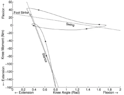
By plotting the knee torque with respect to the angle one can have a perception of how does the knee stiffness (slope of the curve) proceeds during gait cycle. One example of such relation is presented in figure 2.8. It is worth notice the knee spring like behavior

(31)

during the stance phase, being the stiffness represented by a uniform spring.

Figure 2.8: Torque-angle of the biological knee during walking. Linear regression during stance and swing phase. [9]

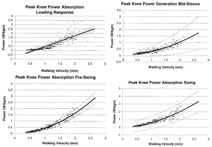
Walking velocity also changes the knee joint torque profile, however, instead of that profile, it is shown in figure 2.9 the peak knee moment during loading response, terminal stance, pre-swing and swing, and its evolution with the walking speed.

(32)

Figure 2.9: Top left : Peak Knee Flexion Moment at Loading Response ; Top right: Peak Knee Extension Moment at Terminal Stance ; Bottom left: Peak Knee Flexion Moment at Pre Swing ; Bottom right: Peak Knee Extension Moment at Swing. [21]

Knee power

The knee power is calculated using equation 2.1 and its profile during the gait cycle with three different velocities is presented in figure 2.10

(33)

Figure 2.10: Knee power profile for slow, natural and fast walking velocities. [47]

These power profiles highlight three main regions of negative power being the first (K1) one related to the loading phase where energy absorption occurs due to the center of mass fall. The other regions are during pre- swing (K3) and finally in terminal swing (K4) to decelerate the moving limb. K2 region corresponds to positive power during mid stance.

It is also possible to represent the peak knee power in loading response, mid-stance, pre-swing and swing, with respect to the walking speed - see figure 2.11

(34)

Figure 2.11: Top left : Peak power at Loading Response ; Top right: Peak power at Mid Stance ; Bottom left: Peak Knee power at Pre Swing ; Bottom right: Peak Knee power at Swing. [21]

As one can see the peak powers in each region increase with the walking velocity.

Regarding the actual work done by the lower limb muscles during one gait cycle, [30], states that stance phase only, accounts for 79.6% ± 7.5 for young and 68.2% ± 3.4 of the total energy. Such fact supports the aim of the thesis, desiring to reduce muscle work during loading response.

(35)

3. Exoskeletons for the Lower Limb

In this chapter a brief context about exoskeletons will be presented to the reader, regarding the several criteria that allow us to classify the types of exoskeletons, as well as the applications range where such can be found.

3.1 Introduction

The word, Exoskeleton, has different definitions depending on the authors. The one adopted was the following, ”mechanical devices that are essentially anthropomorphic in nature, are worn by an operator and fit closely to the body, and work in concept with the operator’s movements.” [16] Generally exoskeleton is a term used for devices that augment the performance of an able-bodied wearer and can be applied in different fields. [16] Such fields include the military one, where this devices are used to reduce soldiers muscle fatigue under load carriage, Human Universal Load Carrier is one of such example. In the industry environment, workers may have to perform activities in harmful position for their joints and muscle, so exoskeleton are indeed useful in order to allow ergonomic postures during work, especially if these ones involve carrying heavy loads. Companies like Panasonic, BMW and Audi already have exoskeletons that help workers during their job activities. [18] The other exoskeleton market is the medical one, more specifically for rehabilitation and augmentation purposes. In the first one the user is assumed that will improve performance with time and so, the exoskeleton support will decrease, though augmentation devices are for individual with chronic motor limitations. Ekso GT and REX are respectively one example of such exoskeletons.

3.2 Exoskeletons taxonomy

The exoskeleton can be divided in different categories based on several properties that will be presented below. First the exoskeleton can be attached in the upper limb (arms and torso), lower limb (hip, knee and ankle joints) actuating in one or several joints at the same time, or in all body. The existence or absence of power is also an important parameter. [23]

(36)

Active exoskeleton can be defined as a wearable system provided with an actuator (hydraulic, pneumatic, electrical motor) capable of increasing the strength and endurance of the human limb. [6] In the other end, the passive exoskeleton, are the ones that do not possess any power source, and usually have springs to store and release energy during the gait cycle, or dampers to dissipate it. The called quasi-passive use a passive actuation system however, are provided with a power source to feed electronic components. An example of such devices is the commercial available C-Brace by Ottobock, witch have a variable damping system incorporated. Lastly, there are the hybrid-exoskeletons that contain a power source used to create Functional Electrical Stimulation which consists on electrical impulses that contract the user muscles. [23]

Regarding the control features, the exoskeleton can have a joystick (for devices that provide 100% of the motion energy); buttons or control panels usually for exoskeletons with pre-programmed modes; electrode skull cap allowing for mind control activation; sensors that monitor linear and angular acceleration, tilt angle, pressure, torque and even Electromyography signals. In the passive exoskeletons the most common is the absence of a control method. [23]

According to the building material there are two main groups, the rigid exoskeletons, built in metallic or low weight fiber-reinforced composite, and the soft exoskeleton or exosuit, that adjust tightly to the user limbs. [23]

Exoskeletons can also be divided depending whether it is in series or parallel with the limb. In the first one, loads are still totally carried by the user joints, nonetheless parallel solutions allows to reduce those loads. [23]

In the scope of this thesis only passive, in series and parallel lower limb exoskeletons will be treated.

(37)

4. Passive Mechanisms of Assistive devices

for Locomotion

In the next chapter some passive exoskeletons mechanisms and results will be pre-sented. Besides, it is also worth pointing out other passive systems, implemented in above knee prostheses, whose purpose is clearly different from the exoskeletons’ one, however the mechanism principle are of interest.

4.1 State of the Art in Passive Exoskeletons

4.1.1 Series-limb exoskeleton

Ligaments and tendon are a biological strategy to reduce impact energy losses while storing some of it when striking the ground and propel the body during late stance in walking and running. This biological structures served as an inspiration for mechanical devices acting in series with the human leg. The first example of this type is the running shoe called Springbuck,figure4.1(a), with a carbon composite elastic midsole that showed some minor metabolic improvements (∼ 2%). Other efforts have been made to improve running speed and economy by devices like the PowerSkip and the SpringWalker, figures 4.1 (b) and 4.1 (c) respectively. Nevertheless, despite this systems clearly augmented jumping height, they did not brought any benefits to locomotion economy. In fact the SpringWalker increased metabolic cost by 20% compared to walking without the device. Results which can be explained by the substantial weight increase to the human leg, requiring more work to be done by the hip to propel the limb during aerial phase. [16]

(38)

Figure 4.1: a) Springbuck ; b) PowerSkip c) SpringWalker. [16]

In series exoskeletons still cause the ground reaction load to be transferred to the human leg. However, by using a parallel exoskeleton this reaction can be held by the device only, resulting in a decrease of the limb loads and metabolic cost, both in walking and running. Furthermore the limb length would not be increased so energy doesn’t need to be spent in movement stabilization. [16]

4.1.2 Parallel-limb exoskeleton

The first mention of such devices is in an America patent granted by Nicholas Yagn in 1890, whose invention is presented in figure 4.2a). This is composed of two long leaf springs operating in parallel to the legs, each supposed to engage during the heel strike, transferring the body weight to the ground and reduce the loads in the limb. The disengagement happened right before the aerial phase in order to allow the leg to flex and gain toe clearance. Until now, there was no record of a built design and it’s demonstration.

(39)

Figure 4.2: a) Yagn’s running design [16] ; b) MIT’s hopping exoskeleton. [15]

MIT biomechatronics group based on the design presented above, built an elastic exoskeleton (figure 4.2 b), which obtained satisfactory results. Unlike the other, whose purpose was to augment running, this was for lowering the metabolic cost. The princi-ple was quite similar, two fiberglass leaf springs spanning the entire leg are capable of transferring body weight directly to the ground during stance period. The MIT device however cannot disengage the spring during aerial phase as it doesn’t contain a clutch device to do so. Even though 24% metabolic cost reductions were reached when compared to normal walking. [15] Such value is hypothesized to be due to low activation of ankle plantar flexors and knee extensors. [9] Nevertheless the lack of a clutch resulted in an expenditure of energy in swing phase as the knee flexion compressed the spring. Later on, MIT also improved this concept by adding a custom high torque and low mass clutch as the commercial options do not fulfill both the requirements for this applications. This clutch (illustrated in figure4.3) has a sawteeth shape with a limiting torque of 190Nm and weights 710g. The implementation of a planetary gear in the device allowed for a torque reduction in the clutch shaft, improving also the angular accuracy on engagement and allowing to machine smaller teeth. Other important feature is the usage of an encoder and a sagital plane gyroscope that are the input elements for the state machine

(40)

algo-rithm capable of identifying the gait cycle stages and de/activate the clutch according to those. In terms of power consumption the total amount of electronic components require 860mW. [9]

Figure 4.3: Mechanism simplified scheme. [9]

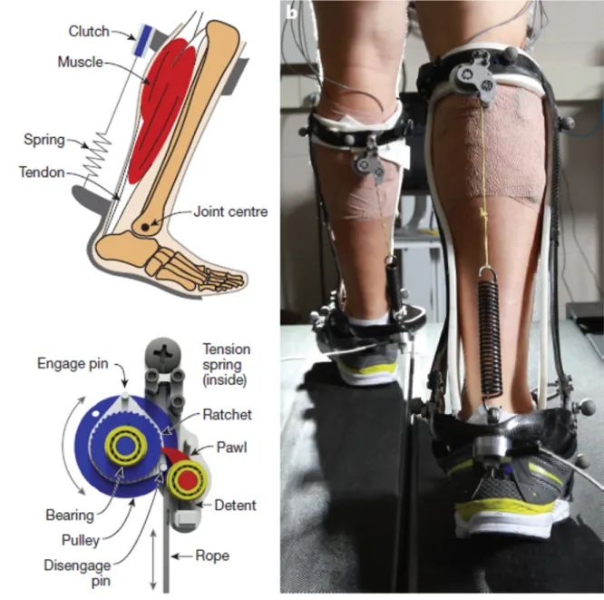
Other investigations were also made in the field of elastic passive exoskeletons with positive results achieved. As a first example, the work of [5] will be summarized. The final goal of the project was to reduce the human walking cost by an unpowered exoskeleton. Figure4.4 demonstrates the device being used, a drawing of the parts and the clutch sys-tem. The main components of the device is a spring parallel to the Achilles tendon, whose function is to reduce calf muscle activation, and a passive clutch whose dis/engagement allows the first element to store and release energy in the right gait cycle stages. At heel strike the clutch was engaged, allowing for the spring to be loaded during the stance phase and then release all that potential energy at toe-off, giving auxiliary torque at the ankle and reducing musculotendon work. Several trials were made varying the spring stiffness and it’s important to remark the non linear relation of metabolic rate with stiffness, be-ing the first reduced until a certain value of stiffness and then increases, evolution seen in figure 4.5. This increasing values might be explained by a higher plantarflexor activity, due to a rise in contraction velocities, in the end of end stance, even though the torque

(41)

produced by this muscles decreased. Actually the metabolic rate increment can not be explained using mechanical power, because human contributions decreased with stiffness raise, nevertheless the metabolic rate increased. [5]

Figure 4.4: Right: User wearing the device ; Top left : Schematic picture with the device elements (Spring and clutch) and their assembly location ; Bottom left : Clutch components. [5]

(42)

Figure 4.5: Metabolic rate evolution with spring stiffness. [5]

The clutch mechanism is worth a deeper look. The diagram in figure 4.6 is helpful to visualize the mechanism in action.

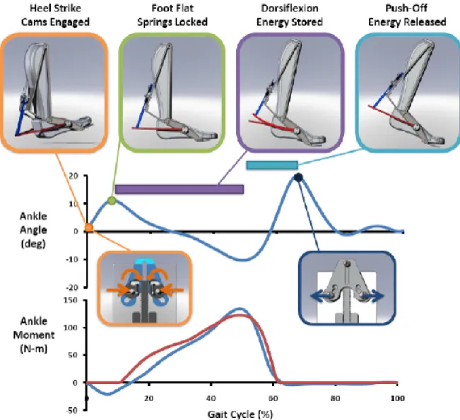
During swing the linkage (Kevlar strands plus linear spring) is allowed to move cre-ating a rotation of the ratchet, motion which is represented as blue arrow lines in the figure. At heel strike (box in orange) however, a pin engages the pawl in the ratchet, re-stricting further downward motion of the linkage. As the foot plantar flexes until foot-flat position (box in purple) the linkage gains slack because of shortening distance between the two connection points. This situation inverts in mid stance as dorsiflexion begins but the clutch is engaged not allowing linkage motion and so the ratchet rotation. System responds by stretching the spring and so energy from the body’s center of mass is stored (green rectangular area). At push of, all the energy previously stored returns to the ankle joint to perform positive mechanical work, resulting in forward body propelling (dark blue rectangle). During the energy release, because of the teeth ratchet shape that only allows unidirectional locking, this part rotates counterclockwise and at maximum plantar flexion other pin now disengages the pawl freeing the ankle to dorsiflex during the rest of swing, resetting the cycle. [46]

(43)

Figure 4.6: Schematic highlighting the key events of the clutch functioning over the gait cycle. The ankle joint pattern (blue line) is from a walking speed of 1.25m/s. Positive values indicate plantarflexion and negative dorsiflexion. [46]

Other similar design is presented in [5], where a leaf spring was used instead with an equivalent stiffness of 5N m/deg and a clutch mechanism based on cams to dis/engage the spring. Figure 4.7 shows the several key points trough the gait cycle. The system is very identical to the previous so it will not be further analyzed. [45]

(44)

Figure 4.7: Schematic highlighting the key events of the clutch functioning over the gait cycle. The ankle joint pattern (blue line) is from a walking speed of 1.25m/s. Positive values indicate plantarflexion and negative dorsiflexion. Ankle moment blue curve is also for a walking speed of 1.25m/s as the red one represents the torque contribution of the spring exoskeleton. Orange outline panels cam/clutch engagement at heel strike. The purple bar indicates the spring storing energy period and the light blue the period of energy release tduring push-off. Dark blue panel illustrate cam/clutch disengaging the spring to allow free swing. [45]

In [42], is presented a quasi-passive exoskeleton (power is used for electronic compo-nents only) for metabolic reduction of walking while carrying a load. The device presented in figure 4.8 is composed of two parallel legs that transfer payload forces to the ground. For energy storage, two springs are employed in the hip and ankle. To ensure knee muscu-lar effort reduction during early stance, a variable damping is implemented. This variable damping was a commercial one made by ¨Ossur of Reykjavik, Iceland. The human inter-face is made by means of a backpack shoulder straps, a waist belt, thigh cuffs and cycling shoes. Regarding the DoFs, the hip joint has three in order to mimic the biological ball

(45)

and socket joint, both knee and ankle have one DoF. The exoskeleton ground interface is made by a carbon fiber foot-ankle produced by the same company as the variable knee damper. [42]

Through experimental trials of a person carrying a 75lb (34Kg) payload it was pos-sible to conclude that the device actually increased metabolic cost by 39% compared to carrying the same weight without the exoskeleton. However by removing the variable damping knee and replacing it by a simple pin joint, the metabolic cost reduced 34% in the same testing conditions. One can hypothesis that the damping advantages are overtaken by the adding mass. The influence of this adding mass is greater as this moves distal to the hip joint, increasing the moment of inertia relative to this joint requiring more torque in order to swing the leg. [42]

Figure 4.8: Picture of exoskeleton being worn and it’s main parts. [42]

Although positive results have been presented, that is not always the case as it can be seen in [43]. In this article a passive exoskeleton named XPED 2 (figure 4.9) was studied. This one uses the concept of exotendons, which are basically long elastic cables spanning multiple joints. This cables act just like a spring, storing and releasing energy between joints. Figure 4.9 a) illustrates the working principles enumerating the several

(46)

components, being the main functional one the exotendon 3), a cable that spans between a lever at the pelvis 1), via a pulley at the knee 4), to a leaf spring at the foot 5) which gives elasticity to the mechanism. Because of the cable’s offset relatively to the joint centers, the spring deformation and so the force acting on the cables will depend on the joint angles. Hip extension and ankle dorsiflexion will tighten the cable and hip flexion and ankle plantarflexion will loosen the cable. In some joint angle combination the cable will be slack meaning no forces on it. The moment on each joint is a simple multiplication of the cable’s force and the joint offset. Human-exoskeleton interface is made by a rigid frame 2) connected to the pelvis, shank and foot segments. In figure4.9 b) the several XPED 2 DoF are highlighted by arrows, showing that six are active per leg. This ones are flexion/extension, ab/adduction and endo/exorotation at the hip, flexion/extension at the knee, plantar/dorsiflexion and pronation/supination at the ankle. [43] The exoskele-ton experiments lead to conclude that although hip and knee kinematics were almost unchanged compared to walking without the device, the same was not applied to the ankle, where the maximum dorsiflexion angle decreased 5◦ compared to normal locomo-tion condilocomo-tions. Regarding the metabolic cost there was an indicalocomo-tion that this actually increased (figure 4.10) although the human joint torque was indeed reduced. In fact ten-dons are already biological energy transfer mechanism and the addiction of exotenten-dons might interfere with this saving systems, increasing the locomotion metabolic cost. Other justification is the substantial leg weight increase, due to the 6.92Kg distributed through the lower limb. [43]

Figure 4.9: a) Working principles ; b) Active degrees of freedom (DoF) ; c) User wearing XPED 2. [43]

(47)

Figure 4.10: The metabolic cost: The bars represent the average over the subjects with the standard deviations.The no support 1 and 2 are the first and second test respectively with the worn exoskeleton without the springs attached. The support 1 and 2 are the first and second test respectively with the worn exoskeleton when the springs are attached. [43]

4.1.3 Passive exoskeletons overview

Table 4.1: Passive exoskeletons overview. Negative values for the metabolic reduction indicate a metabolic increasement, and vise-versa.

Name Spring Damper joints Metabolic reduction

Series Springbuck [16] × +2% PowerSkip [16] × – SpringWalker [16] × -20% P arallel

MIT’s hopping [9] × Knee +24%

Unpowered Exo. [5] × Ankle +7.2%

Leaf spring [45] × Ankle –

Load carry [42] × × Ankle/Knee/Hip +34%

(48)

Every system analyzed, except one, relied on the use of a spring to store and release energy. Indeed, as mentioned in section 2.3.1, the knee has a spring-like behavior in the stance phase, commonly motivating the usage of a spring mechanism.

On the other hand, considering the full gate cycle, this joint has three time-intervals of energy dissipation, which resembles the behavior of a damper. This thesis took this consideration, following a different approach of the most used in the state of the art. In fact, only one exoskeleton (for the knee) was found using a damper, but, firstly, it did not have a beneficial result [42] and, second, an expensive and too complex damper was selected, while this thesis proposes the design of an economical mechanism.

4.2 Other passive mechanisms – Knee Prostheses

Knee prostheses mechanisms also use passive elements like springs or dampers in order to fulfill their use. Springs solutions have already been presented so more focus will be given to the damper systems. This operate using fluids in liquid or gas states, that dissipate the energy via viscous motion resulting then in an increment of the fluid internal energy. The system can be described as a simple dash-pot where the holes function can be replaced by valves with a variable or static displacement depending on the solution complexity. The first type are capable of changing the damping coefficient, depending on the velocity and also the gait cycle stage. An example of such devices is presented below being applied in a transfemoral knee prosthesis.

The damper, whose explication follows, is a pneumatic swing-control above knee prosthesis whose main goal is control the shank motion during this gait cycle stage. For that purpose a double pneumatic actuator with three valve step up was built, being two of those bidirectional flow control valves, L and R and one check valve. The flow control valves also called leak rate valve are a crucial component being responsible for the damping and elastic effect on the system. If closed the devises behaves as a pneumatic spring and so the energy is stored and is only a function of position, meanwhile if opened the air will flow from the pressurized chamber to the other resulting in an exchange of mass. In the end most of energy is dissipated through heat by an increase of the air internal energy. Also important to remark that the Pressure-displacement evolution is now highly dependable with the piston velocity and the valve opening. The relation curves differ from the pneumatic spring being this values lower as the valve opening increases. [19]

(49)

Figure 4.11: Right: Air flow corresponding to knee flexion ; Left: Air flow corresponding to knee extension. [19]

During initial swing the knee flexes and from the actuator view point, a high pressure is built in the lower chamber and air flow is made trough L valve,witch is the dominant damping element in this phase, to the too chamber. When maximum flexion angle is reached the pressure difference between the chambers might not be reestablished due to the low flow valve opening or the high velocities. The consequence is an initial thrust in extension motion, however as it progresses the top chamber is pressurized and flow is made from top to bottom, though this time the check valve opens and both L and R valves serve as path for the air reducing the motion resistance. During stance phase the pressures on the chambers are equalized and prepared for other duty cycle. [19]

(50)

5. Knee damping coefficient estimation

5.1 Gait data analysis

When designing a passive system, it is necessary to know the required knee damping coefficient for different walking speeds. However, these values are hard to generalize for different subjects as the damping coefficient changes with their leg length and weight. Still, one can estimate such values for an average person. So, the joint Kinematics and Kinetics data from a 70Kg male individual with a leg length of 90cm, walking at 0.5, 1 and 1.5m/s [48] were analyzed and the extracted coefficient used as reference for the design.

The knee angle, velocity, torque and power are plotted in figure5.1. It is important to state that the data presented, expect for the angular velocity, resulted from a polynomial fit to the original data. The coefficient of determination, R2 for each fit is shown in table 5.1.

Table 5.1: Polynomial fits.

Velocity (m/s) 0.5 1.0 1.5 Polynomial Degree 18 13 15 Knee Angle R2 _1.0000 _0.9999 _0.9999

Knee Moment R2 0.9991 0.9926 0.9984 Knee Power R2 _0.9951 _0.9897 _0.9951

The angular velocity was obtained using two consecutive times and also the differ-ence of the knee angle at each time considered. Equation 5.1 translates this relation mathematically. ˙ θi = θi+1− θi ti+1− ti (5.1)

With the polynomial fit instead of the 50 points available in the original data one can have as many points as desired, which allowed a more precise calculation of the angular velocity.

(51)

0 20 40 60 80 100 % of gait cycle 0 20 40 60 Knee angle [ ° ] Knee Angle 0 20 40 60 80 100 % of gait cycle -400 -200 0 200 400 600 Knee Velocity [ ° /s] Knee Velocity 0 20 40 60 80 100 % of gait cycle -20 0 20 40 60 Knee Moment [Nm] Knee Moment 0 20 40 60 80 100 % of gait cycle -100 -50 0 50 100 Knee Power [W] Knee Power 0.5 [m/s] 1 [m/s] 1.5 [m/s]

Figure 5.1: Kinematic and Kinetic data at three different walking speeds (0.5, 1.0, and 1.5m/s).The lines are the curve fitting result and the dots represent the data used to make them. 0 10 20 30 40 50 60 70 80 90 100 % of gait cycle -50 0 50 Knee Power [W] 0.5 [m/s] [1] [2] 0 10 20 30 40 50 60 70 80 90 100 % of gait cycle -50 0 50 Knee Power [W] 1 [m/s] [1] [2] 0 10 20 30 40 50 60 70 80 90 100 % of gait cycle -100 -50 0 50 Knee Power [W] 1.5 [m/s] [1] [2]

(52)

It is, then, necessary to know, for each speed trial, which region corresponds to K1. This was done by simply identifying the points where the Knee power profile is zero. The region of interest is between the first and second point as indicated in figure 5.2.

Having the K1 region defined one can obtain the damping coefficient evolution with respect to the knee angle (represented in figure5.3). This parameter is calculated in each point by doing the division below:

Ci =

τi

˙ θi

(5.2)

where Ci, τiand ˙θiare the damping coefficient, the knee moment and the knee angular

speed at each point i, respectively.

3 4 5 6 7 8 9 10 11 12 % of gait cycle 0 20 40 0.5 [m/s] 3 4 5 6 7 8 9 10 11 12 % of gait cycle 0 20 40

Damping Coefficient [Nm.s/rad]

1 [m/s] 3 4 5 6 7 8 9 10 11 12 % of gait cycle 0 20 40 1.5 [m/s]

Figure 5.3: Damping coefficient for the three velocities during the K1 region.

As the gait cycle develops, the damping coefficient tends to infinity, because of the zero angular velocity reached at the end of K1, which corresponds to the angular peak during the loading response. Consequently, in the figure above (5.3), the plot was limited to 50N.m.s/rad, in the y-axis, because the very high damping coefficients close to the end of K1 (≈ 12%) did not allow the smallest values to be visible.

(53)

An alternative to visualize the data is to plot the knee moment with respect to the angular velocity. The results are presented in figure 5.4.

10 20 30 40 50 60 70 Angular velocity [°/s] -20 0 20 Velocity 0.5 [m/s] P_beginPInversion P ending 0 10 20 30 40 50 60 70 80 90 100 Angular velocity [°/s] -50 0 50 Knee Moment [Nm] Velocity 1 [m/s] P begin P Inversion P_ending -50 0 50 100 150 200 250 Angular velocity [°/s] -50 0 50 Velocity 1.5 [m/s] P begin P Inversion P ending

Figure 5.4: Knee Moment with respect to the angular velocity.

A very important observation results from this analysis: biologically, some velocities are associated with two different values of moment. However, for a device to reproduce this behavior, the damping coefficient would have to change dynamically during the gait cycle, requiring an extra system to induce that modification and, consequently, increasing the complexity of the device. As a first approach, a simpler system is desired, so, in this thesis, the damping mechanism was considered to be only changeable before start walking.

5.2 Damping coefficient estimation

A very simple approach is done in order to find a suitable reference value for the damping coefficient. For each walking velocity the following calculations are performed.

(54)

EK1= Z t(Pending) t(Pbegin) CDamper∗ ˙θ2dt (5.3) Z t(Pending) t(Pbegin) WKneedt = CDamper∗ Z t(Pending) t(Pbegin) ˙ θ2dt (5.4) CDamper = Rt(Pending) t(Pbegin) WKneedt Rt(Pending) t(Pbegin) ˙ θ2_dt (5.5)

Basically, CDamper is found integrating the given knee power, and the knee angular

speed squared. Table 5.2 indicates the calculated values for this parameter. Indeed the results are odd because there is not a continues growth of the damping coefficient with the walking velocity, making the calculation method not trustworthy (too simplistic). Nevertheless this data is still used.

Table 5.2: Damper coefficient values for each walking velocity studied.

Walking Velocity 0.5m/s 1m/s 1.5m/s CDamperN.m.s/rad 5.72 14.41 7.93

Following this, the real knee torque can be compared with the one created assuming the calculated damper coefficients, if the kinematic profile for each walking speed is used. The result is presented in figure 5.5.

As one can see, in the beginning of region K1, the damper moment is bigger than the real knee moment, leading to the conclusion that a kinematic change will occur in the knee. In addition, the constant damping consideration approximates the real knee moment poorly, yet, allows to have some reference numbers for that characteristic.

(55)

3 4 5 6 7 8 9 10 11 12 13 Gait cicle

-20 0

20 0.5 [m/s]

Real knee moment

Damper moment contribution

2 4 6 8 10 12 14 Gait cicle -50 0 50 Knee moment [Nm] 1 [m/s] 2 4 6 8 10 12 14 Gait cicle -50 0 50 1.5 [m/s]

Figure 5.5: Comparison of the real knee moment with the one produced by the calculated damper coefficients for the three different walking velocities.

5.3 Conclusion

In this chapter, a gait cycle at three different walking speeds was evaluated, to ad-dress some reference values desired for the damping coefficient of the device’s damping mechanism. This analysis showed a high variation of such coefficient with the walking speed, implying that, ideally, the selected damper should be tuneable, ranging its coef-ficient from 5.72 to 14.41 N.m.s/rad. Of course these values are obtained from data of one person only, being subjected to error both in data acquisition and post-processing. Still, these are useful to gain sensibility to this coefficient value, even tough it can poorly reproduce the real knee moment,5.5. So, the damper selected in chapter7should have a damping coefficient between 5 and 15N.m.s/rad.

(56)

6. Solution 1 - Pneumatic actuator

This system is meant to have a pneumatic actuator connected to the thigh and shank. By using a restriction valve that allows communication between the two chambers, air flow would suffer a resistance and energy would be wasted in the form of heat. A by-pass would be required to free the system, so that the user could move the limbs, ideally with null resistance in specific gait phases.

This chapter offers a theoretical and preliminary analysis, as rigorous data for the valves were not found, and, consequently, values of some parameters had to be assumed.

6.1 System overview

For the system to be able to properly provide the required knee torque, some in-ternal pressure, bigger than the atmospheric one, must exist. This unknown pressure is determined in section 6.2 based on a subject’s kinematic and kinetic data from several walking speeds (addressed in chapter 5). The pressure must be held in the system, and for that, the two chambers must be connected and isolated from the outside. Besides this, the effective chamber area must be the same, otherwise, with the same pressure on both sides, the forces transmitted to the limb segments would be different, causing distortions in the walking pattern. The conclusion taken is the need for a symmetric chamber area, leading to the use of a through-piston-rod pneumatic actuator. To actually dissipate en-ergy, a restriction flow valve is used, being regulated according to the person and his/her walking speed. However, it is only supposed to be active during the K1 region. After that, a parallel system must deviate the air flow from the restrictor, making the device transparent to the user. Such flow change is done by a 5/2 pneumatic solenoid valve, that when piloted can direct the flow from one chamber directly to the other reducing the pressure difference between them (so the system resistance), or force the air through the unidirectional flow restrictor valve (UFRV). The other valve, a 2/2 normally closed (NC), is used so that air can fill the chamber and remain in the pneumatic circuit.

(57)

Figure 6.1: Pneumatic circuit and its components.

Regarding the connections to the limbs, the actuator rod can be linked, for example, to the shank, forcing the actuator body to be locked to the thigh. This strategy will result in the movement of the other rod during the gait cycle, and special attention must be taken to avoid this moving rod to touch the human body. The actual interface between limbs and actuator is not studied here, but figure6.2demonstrates an example of an active knee exoskeleton whose limb connections can be applied to this pneumatic solution.

(58)

Figure 6.2: Lower Limb Exoskeleton KIT-EXO-1. An example regarding the actuator-limb in-terface. [3]

In the next paragraphs, the system usage in each phase of the gait cycle will be explained in detail:

At the heel strike instance, the actuator starts to compress, meaning air flows from chamber A to B (see 6.1). In this stage, the air path must cross the UFRV, responsible for damping the motion, and, to do so, the 5/2 valve must be switched. After the peak knee flexion during the loading phase, the directional valve returns to the original position, making the system transparent. Note that the directional valve must have two blocked ports so that air does not leave the system. Although such valve configuration behaves as a 3/2 valve, that cannot be used, as port 3 is not accessible, unlike a 5/2 valve, where all ports are available for connections.

Table 6.1 summarizes the system resistance or transparency depending on the actu-ator’s direction of motion (extending or shortening) and the state of the 5/2 valve (active or inactive).

(59)

5/2 state Actuator motion Inactive Active Extending (B-A) Transparent Transparent Shortening (A-B) Transparent Resistance

Table 6.1: Inactive and active refer, respectively, to the normal position and the position when the solenoid is activated. The actuator direction of motion is characterized by the air flow direction, A-B or B-A, where the first letter indicates the source chamber and the last the destination chamber.

In the event of lack of power (5/2 is inactive), for safety reasons, the user’s locomotion must not be affected. For that purpose the device only resists motion when the solenoid from the directional valve is activated.

6.2 Actuator Selection

The methodology to select the actuator dimensions and internal pressure were based on the hypothesis of the actuator’s chambers being completely isolated from each other, having then a pneumatic spring. Moreover, this spring can be analyzed as an adiabatic system because the K1 region accounts roughly for 12% of the gait cycle, lasting a few hundred of milliseconds [34], time in which the effects of thermal dissipation through conduction and convection are negligible.

The adiabatic pressure evolution in a chamber is given by equation 6.1.

P2 = Pi

Lic

Lc

!γ

(6.1)

P2 refers to the air pressure in the compression chamber, whose length is Lc. Pi

and Lic represent, respectively, the initial pressure and initial chamber length. γ is the

adiabatic constant, which for air can be considered 1.4 [28].

The installed pressure will then produce a force proportional to the chamber’s area, which will then cause a moment in the knee joint. The main goal is to approximate this moment of force to the biological muscle torque in the knee during the loading phase, so that less energy is wasted by the muscles. However, first, it’s necessary to evaluate the

(60)

stroke of the actuator, that will depend on where it is attached, and then estimate the required chamber area as well as the initial pressure, Pi.

A limiting value for the minimum stroke (St) of the actuator can be found considering the model presented in figure6.3. The actuator is connected to the thigh and shank along the axis created by straight lines joining the hip-knee and knee-shank joints. The top end of the actuator is fixed with a distance Xk from the knee. The bottom end is Xs distant from the same joint. Finding the minimum stroke consists in determining the maximum length variation of the actuator during the gait cycle.

Figure 6.3: Simple model to determine the actuator minimum stroke.

The actuator length, La, can be defined with respect to Xk, Xs and the knee angle θk by applying the law of cosines, as in equation6.2.

La2 = Xk2+ Xs2− 2 ∗ Xk ∗ Xs ∗ cos(π − θk) (6.2)

(61)

St = Xk + Xs − v u u tXk2+ Xs2− 2 ∗ Xk ∗ Xs ∗ cos π − θkM ax ∗ π 180 ! (6.3)

Evaluating the evolution of this parameter, with Xk and Xs comprised between 100 and 500mm, generates the surface presented in figure 6.4.

50 500

100 150

St (Minimum stroke) distance

400 Xk distance 300 Evolution of St 200 100 150 Xs distance 200 250 300 350 100 ₄₅₀ ₄₀₀ 500

Figure 6.4: Minimum actuator stroke evolution. The black dots indicate the maximum evolution of St.

As one can see, St assumes higher values when Xk and Xs are equal (black dots in the figure above).

Now that the stroke dependency on Xk and Xs is well defined, the next step requires an actuator to be chosen, and knowing its stroke values, Xk and Xs can be set. These two variables are essential as they dictate the pressure evolution inside the actuator when it behaves as a pneumatic spring. In fact, the pneumatic spring consideration is just a simplification to find an appropriate internal pressure. In reality, any pressure curve

(62)

the restrictor valve. One can see a pneumatic spring as a restrictor valve with infinite flow resistance.

Several through-piston-rod pneumatic actuators from Festo, were considered, having a stroke (StA) of 50, 75, 80, 100, 125, 150, 160, 200, 250, 300, 320, 400 and 500mm. The

actuators chosen have a chamber outer diameter (Dext) of 32mm, a 12mm rod diameter

(Drod) and a maximum pressure operation of 10bar and an effective chamber diameter of

30 mm. [10]

Equations 6.4 and 6.5 allow us to calculate Xk and Xs, which are the same, by knowing the actuator stroke, StA.

StA = Xk + Xs − v u u tXk2+ Xs2− 2 ∗ Xk ∗ Xs ∗ cos θkM ax ∗ π 180 ! (6.4) Xk = Xs (6.5)

The evolution between StAand the calculated Xk and Xs are illustrated in figure6.5

50 100 150 200 250 300 350 400 450 500 Stroke [mm] 0 200 400 600 800 1000 1200 1400 Xk and Xs [mm]

Figure 6.5: Relation between Xk and Xs with StA.

A visual meaning of the value Xk and Xs can be seen in figure 6.6. The crosses represent the place where the mechanical connections to the limb interface mechanism should be.

(63)

Figure 6.6: Visual representation of the Xk and Xs values. The crosses represent the place where the mechanical connections to the limb interface mechanism should be.

6.3 Initial Pressure

Kinetic and kinematic data from a 70Kg male, walking at three speeds, 0.5, 1 and 1.5m/s were used to predict a reasonable value for the initial pressure, Pi, in the actuator,

so that the spring-like behavior approximates the real knee moment. More information about this gait data analysis can be seen in chapter 5.

To compute the initial pressure, Pi, a linear regression was made, in which the input

(X) was obtained as below. The output (Y) is simply the knee moment from the given data. X = Bj ∗ Aef t∗   Lic Lc !γ − Lie Le !γ  (6.6) Pi∗ X = Y (6.7)

Note that Pi is the coefficient that minimizes the root mean square error between

X ∗ Pi and the output Y.

Bj is the lever arm for the actuator force, at the time j, with respect to the knee

joint - see figure 6.7. This actuator force is produced by the actuator shortening during the K1 region. Lic, Lc, Lie, Le are the initial length of the compression chamber, the compression chamber length throughout K1 phase, the initial length of the expansion

(64)

Figure 6.7: Bj is the minimum distance between the knee joint and a perpendicular line to the

actuator (line in red).

Such procedure was repeated for each walking speed and stroke value, resulting in the graphs presented in figure 6.8.

50 100 150 200 250 300 350 400 450 500 Stroke [mm] 0 2 4 6 8 10 12 14

Initial pressure [bar]

0.5 [m/s] 1 [m/s] 1.5 [m/s]

Figure 6.8: Initial pressure values, in bar, depending on the actuator stroke and walking speed.

(65)

maxi-mum limiting pressure of 8bar [12]. With this said, 8 bar must be the maximaxi-mum allowable pressure in the compression chamber. Figure 6.9 indicates the maximum pressure in the compression chamber during the K1 phase.

50 100 150 200 250 300 350 400 450 500 Stroke [mm] 0 2 4 6 8 10 12 14 16

Maximum pressure [bar]

0.5 [m/s] 1 [m/s] 1.5 [m/s]

Figure 6.9: Maximum pressure values for the compression chamber, in bar, depending on the actuator stroke and walking speed.

So, based on the figure above, to have the minimum weight possible and still fulfill the required limiting pressure of 8 bar, a stroke of 100mm must be chosen, making Xk and Xs equal to 276,48mm (equation 6.4), and Pi equal to 6.9bar (figure6.9). The actuator,

alone, weights 525.5g. [10]

Figure 6.10 illustrates the difference between the moment created by the selected pneumatic actuator (when performing as a pneumatic spring) and the real knee moment, during K1, for a walking speed of 1.5m/s. As one can see, the actuator mimics fairly well the biological knee moment only assuming higher values in the end of K1, with 4Nm difference between the peaks of the two functions.

A wearable mechanism to assist the knee during the loading response

Faculdade De Engenharia Da Universidade Do Porto