HESSD
12, 3477–3526, 2015Modelling ecosystem services for
ecosystem accounting
C. Duku et al.
Title Page
Abstract Introduction
Conclusions References
Tables Figures
◭ ◮
◭ ◮
Back Close
Full Screen / Esc
Printer-friendly Version Interactive Discussion
Discussion
P
a
per
|
Discussion
P
a
per
|
Discussion
P
a
per
|
Discussion
P
a
per
|
Hydrol. Earth Syst. Sci. Discuss., 12, 3477–3526, 2015 www.hydrol-earth-syst-sci-discuss.net/12/3477/2015/ doi:10.5194/hessd-12-3477-2015
© Author(s) 2015. CC Attribution 3.0 License.
This discussion paper is/has been under review for the journal Hydrology and Earth System Sciences (HESS). Please refer to the corresponding final paper in HESS if available.
Towards ecosystem accounting:
a comprehensive approach to modelling
multiple hydrological ecosystem services
C. Duku1, H. Rathjens2, S. J. Zwart3, and L. Hein1
1
Environmental Systems Analysis Group, Wageningen University, P.O. Box 47, 6700AA, Wageningen, the Netherlands
2
Department of Earth, Atmospheric, and Planetary Sciences, Purdue University 550 Stadium Mall Drive, West Lafayette, IN 47907-2093, USA
3
Africa Rice Center, 2031 PB, Cotonou, Benin
HESSD
12, 3477–3526, 2015Modelling ecosystem services for
ecosystem accounting
C. Duku et al.
Title Page
Abstract Introduction
Conclusions References
Tables Figures
◭ ◮
◭ ◮
Back Close
Full Screen / Esc
Printer-friendly Version Interactive Discussion
Discussion
P
a
per
|
Discussion
P
a
per
|
Discussion
P
a
per
|
Discussion
P
a
per
|
Abstract
Ecosystem accounting is an emerging field that aims to provide a consistent approach to analysing environment-economy interactions. In spite of the progress made in mapping and quantifying hydrological ecosystem services, several key issues must be addressed if ecohydrological modelling approaches are to be aligned 5
with ecosystem accounting. They include modelling hydrological ecosystem services with adequate spatiotemporal detail and accuracy at aggregated scales to support ecosystem accounting, distinguishing between service capacity and service flow, and linking ecohydrological processes to the supply of dependent hydrological ecosystem services. We present a spatially explicit approach, which is consistent with ecosystem 10
accounting, for mapping and quantifying service capacity and service flow of multiple hydrological ecosystem services. A grid-based setup of a modified Soil Water and Assessment Tool (SWAT), SWAT Landscape, is first used to simulate the watershed ecohydrology. Model outputs are then post-processed to map and quantify hydrological ecosystem services and to set up biophysical ecosystem accounts. Trend analysis 15
statistical tests are conducted on service capacity accounts to track changes in the potential to provide service flows. Ecohydrological modelling to support ecosystem accounting requires appropriate decisions regarding model process inclusion, physical and mathematical representation, spatial heterogeneity, temporal resolution, and model accuracy. We demonstrate this approach in the Upper Ouémé watershed in 20
Benin. Our analyses show that integrating hydrological ecosystem services in an ecosystem accounting framework provides relevant information on ecosystems and hydrological ecosystem services at appropriate scales suitable for decision-making. Our analyses further identify priority areas important for maintaining hydrological ecosystem services as well as trends in hydrological ecosystem services supply over 25
HESSD
12, 3477–3526, 2015Modelling ecosystem services for
ecosystem accounting
C. Duku et al.
Title Page
Abstract Introduction
Conclusions References
Tables Figures
◭ ◮
◭ ◮
Back Close
Full Screen / Esc
Printer-friendly Version Interactive Discussion
Discussion
P
a
per
|
Discussion
P
a
per
|
Discussion
P
a
per
|
Discussion
P
a
per
|
1 Introduction
Ecosystem accounting provides a systematic framework to link ecosystems to economic activities (Boyd and Banzhaf, 2007; Maler et al., 2008; Edens and Hein, 2013; EC et al., 2013; Obst et al., 2013). Specifically, ecosystem accounting aims to integrate the concept of ecosystems services, i.e., the contribution of ecosystems 5
to human welfare (TEEB, 2010), in a national accounting context, as described in UN et al. (2009). There is increasing interest in ecosystem accounting as a new, comprehensive tool for environmental monitoring and management (Obst et al., 2013). The recently released System of Environmental-Economic Accounting (SEEA)-Experimental Ecosystem Accounting guideline (EC et al., 2013) provides guidelines for 10
setting up ecosystem accounts. A key distinguishing feature of ecosystem accounting is the distinction between the flow of ecosystem services and the capacity of ecosystems to provide service flows (EC et al., 2013). Service flow is the contribution in space and time of an ecosystem to either a utility function (e.g. private household) or a production function (e.g. crop production) that leads to a human benefit, whereas service capacity 15
is a reflection of ecosystem condition and extent at a point in time, and the resulting potential to provide service flows (Edens and Hein, 2013; EC et al., 2013).
An issue that is currently unresolved is the incorporation of hydrological ecosystem services into ecosystem accounts (e.g. EC et al., 2013). Hydrological ecosystem services are provided by ecohydrological interactions between terrestrial and aquatic 20
ecosystem components (Brauman et al., 2007; D’Odorico et al., 2010). Hydrological ecosystem services provision underlies water and food security. A variety of approaches have been used to model, map and quantify these services (e.g. Le Maitre et al., 2007; Naidoo et al., 2008; Liquete et al., 2011; Maes et al., 2012; Notter et al., 2012; Willaarts et al., 2012; Leh et al., 2013; Liu et al., 2013; Terrado et al., 2014 for 25
HESSD
12, 3477–3526, 2015Modelling ecosystem services for
ecosystem accounting
C. Duku et al.
Title Page
Abstract Introduction
Conclusions References
Tables Figures
◭ ◮
◭ ◮
Back Close
Full Screen / Esc
Printer-friendly Version Interactive Discussion
Discussion
P
a
per
|
Discussion
P
a
per
|
Discussion
P
a
per
|
Discussion
P
a
per
|
and service flow, and linking ecohydrological processes (and ecosystem components) to the supply of dependent hydrological ecosystem services. Addressing these issues require appropriate decisions regarding model process inclusion, spatial heterogeneity, physical and mathematical representation, temporal resolution, and model accuracy (Guswa et al., 2014). We elaborate on some of these factors below.
5
First, in ecosystem accounting, spatial units form the basic focus for measurement, similar to functions of economic units in national accounting (EC et al., 2013). Adequate representation of spatial heterogeneity of biophysical environment in ecohydrological models is, therefore, crucial. Several types of spatial discretization have been used to represent heterogeneity (e.g. Bronstert and Plate, 1997; Arnold et al., 1998; Manguerra 10
and Engel, 1998; Easton et al., 2008; White et al., 2009; Arnold et al., 2010; Rathjens et al., 2014). Generally, the discretization type has been found not to have any significant effect on aggregated hydrological attributes at a watershed outlet (e.g. streamflow), however, grid-based discretization has been reported to provide a more detailed and accurate spatial description of ecohydrological processes (Arnold et al., 15
2010; Rathjens et al., 2014).
Second, if ecosystem accounting is to provide reliable information for the assessment of integrated policy responses at the landscape level, then physical and mathematical representation of model processes should be based on scientific consensus (Vigerstol and Aukema, 2011). Ecohydrological models, specifically, should simulate the 20
landscape controls on ecohydrological processes and functioning such as hydrological flow paths, water storage and associated transport of sediments and nutrients (Bosch et al., 2010; Tetzlaffet al., 2010).
Third, model results should be accurate and model uncertainties should be understood and reported. Seppelt et al. (2011) and Martínez-Harms and Balvanera 25
HESSD
12, 3477–3526, 2015Modelling ecosystem services for
ecosystem accounting
C. Duku et al.
Title Page
Abstract Introduction
Conclusions References
Tables Figures
◭ ◮
◭ ◮
Back Close
Full Screen / Esc
Printer-friendly Version Interactive Discussion
Discussion
P
a
per
|
Discussion
P
a
per
|
Discussion
P
a
per
|
Discussion
P
a
per
|
to capture these spatial variations increase the uncertainties associated with modelled ecohydrological processes and dependent hydrological ecosystem services produced at subwatershed scales.
Finally, temporal variability in ecohydrological processes cause variations in hydrological ecosystem services provision over time within the same spatial unit 5
(Santhi et al., 2008; Fisher et al., 2009). This can have significant impacts on the type of stakeholders and the values attached to hydrological ecosystem services (Zhang et al., 2013). Continuous simulation watersheds models able to capture short and long-term temporal variability are useful for analysing the temporal scales of service provision.
Our objective, therefore, is to present a spatially explicit modelling approach, 10
which distinguishes between service capacity and service flow, to map and quantify hydrological ecosystem services in order to set up ecosystem accounts. The services we model and account for are crop water supply, household water supply (groundwater supply and surface water supply), water purification, and soil erosion control. In our approach, a grid-based setup of a modified Soil Water and Assessment Tool (SWAT), 15
SWAT Landscape, is first used to simulate the watershed ecohydrology. The model is then calibrated and validated. Model outputs are post-processed based on indicator requirements that are consistent with an ecosystem accounting framework to map and quantify hydrological ecosystem services and to set up biophysical ecosystem accounts. We demonstrate this approach in the Upper Ouémé watershed in Benin. This 20
case-study area was selected because of a relatively high data availability (Judex and Thamm, 2008; AMMA-CATCH, 2014). It is also a microcosm of sub-Saharan Africa, where large sections of the population depend on smallholder rainfed agriculture for their livelihood and where there is increasing land degradation and competition for scarce water resources.
HESSD
12, 3477–3526, 2015Modelling ecosystem services for
ecosystem accounting
C. Duku et al.
Title Page
Abstract Introduction
Conclusions References
Tables Figures
◭ ◮
◭ ◮
Back Close
Full Screen / Esc
Printer-friendly Version Interactive Discussion
Discussion
P
a
per
|
Discussion
P
a
per
|
Discussion
P
a
per
|
Discussion
P
a
per
|
2 Description of case-study area
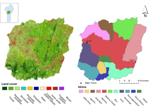
The Upper Ouémé watershed as depicted in Fig. 1 is located in central Benin covering an area of approximately 14 500 km2. The natural vegetation is a mosaic of savannah woodland and small forest islands with a protected forest area of about 2420 km2within the watershed. Smallholder rainfed agriculture is the major economic activity and is 5
supported by suitable climatic conditions that are characterized by a unimodal rainfall season from May to October of about 1250 mm per year. There is low demographic density (28 inhabitants km−2) within the watershed with a population of about 400 000 (Judex and Thamm, 2008). However, the population is growing rapidly (about 4 % per annum) due to migrants coming from different parts of the country and other 10
neighbouring countries to farm. Rapid population growth has caused the expansion of agricultural areas and led to both deforestation and increasing scarcity of agricultural land (Judex and Thamm, 2008) accompanied by increasing soil degradation due to shortening of the fallow period (Giertz et al., 2012). As a result, inland valley lowlands are increasingly converted for crop production due to their higher water availability, 15
lower soil fragility and higher fertility compared to upland areas (Giertz et al., 2012; Rodenburg et al., 2014).
3 Methods
3.1 Modelling watershed ecohydrology 3.1.1 Model selection
20
HESSD
12, 3477–3526, 2015Modelling ecosystem services for
ecosystem accounting
C. Duku et al.
Title Page
Abstract Introduction
Conclusions References
Tables Figures
◭ ◮
◭ ◮
Back Close
Full Screen / Esc
Printer-friendly Version Interactive Discussion
Discussion
P
a
per
|
Discussion
P
a
per
|
Discussion
P
a
per
|
Discussion
P
a
per
|
topography and land management) instead of regression equations (Neitsch et al., 2009), (ii) the ability to calibrate and validate each ecohydrological process (using tools such as Abbaspour et al., 2008), (iii) the daily time-step and continuous simulation that enables the model to capture short and long term temporal variability in service provision, (iv) the ability to simulate the effect of land use change as well as a range of 5
land management options on service provision, and (v) that the model has been tested extensively under varying conditions in different landscapes (Gassman et al., 2007).
3.1.2 From SWAT to SWAT Landscape
In the SWAT model, a watershed can be spatially discretized using three approaches. They are grid cells, representative hillslopes, and hydrologic response units (HRUs) 10
(Arnold et al., 2013). The HRU-based discretization is the most popular and all geographic information system interfaces are set up to use this discretization (e.g. ArcSWAT). Each HRU is a lumped area within a subwatershed that is comprised of unique land cover, soil and management combinations (Neitsch et al., 2009). An HRU does not have a spatial reference in the landscape and there are no spatial interactions 15
among different HRUs in the land phase of the hydrological cycle (Neitsch et al., 2009). Therefore, transported water, sediment, nutrient and pesticide loadings from upstream HRUs are routed directly into stream channels bypassing downstream HRUs (Bosch et al., 2010). This has been identified as a key weakness of the model (Gassman et al., 2007; Volk et al., 2007; Arnold et al., 2010; Bosch et al., 2010; Rathjens et al., 2014). 20
A landscape routing sub-model that simulates surface water, lateral and groundwater flow interactions across discretized landscape units was, therefore, developed and incorporated into the SWAT model by Volk et al. (2007) and Arnold et al. (2010). This modified model, SWAT Landscape model, uses a constant flow separation ratio to partition landscape and channel flow in each HRU (Arnold et al., 2010). However, when 25
HESSD
12, 3477–3526, 2015Modelling ecosystem services for
ecosystem accounting
C. Duku et al.
Title Page
Abstract Introduction
Conclusions References
Tables Figures
◭ ◮
◭ ◮
Back Close
Full Screen / Esc
Printer-friendly Version Interactive Discussion
Discussion
P
a
per
|
Discussion
P
a
per
|
Discussion
P
a
per
|
Discussion
P
a
per
|
flow (Rathjens et al., 2014). A detailed description of the SWAT Landscape model can be found in Arnold et al. (2010) and Rathjens et al. (2014).
3.1.3 Model input data
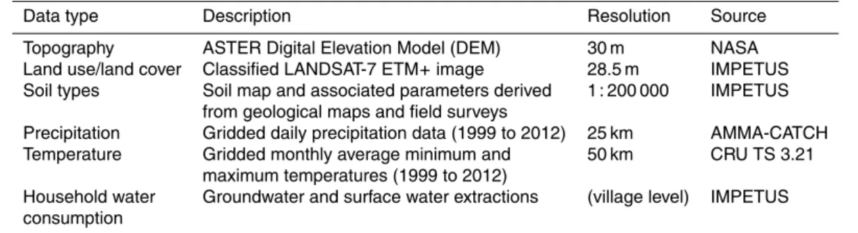
A combination of spatial and non-spatial input data from a variety of sources were used to set up the model. The spatial input data are described in Table 1. A 30 m 5
digital elevation model (DEM) was obtained from the National Aeronautics and Space Administration (NASA) ASTER Global Digital Elevation Map to generate stream network, watershed configurations and to estimate topographic parameters. Land cover and soil maps were obtained from the “Integrated Approach to Efficient Management of Scarce Water Resources in West Africa” (IMPETUS) project database (Judex and 10
Thamm, 2008). The land cover map had been derived from classification of LANDSAT-7 ETM+satellite image. Gridded daily precipitation data were obtained from the “African Monsoon and Multidisciplinary Analysis–Coupling the Tropical Atmosphere and the Hydrological Cycle” (AMMA-CATCH) database (AMMA-CATCH, 2014) and gridded temperature data were obtained from Climate Research Unit (CRU) TS 3.21 database 15
(Jones and Harris, 2013). Data on groundwater and surface water extractions for household consumption were obtained from the IMPETUS project database. These had been derived from national census and household surveys in about 200 towns and communities within the watershed (INSAE, 2003; Hadjer et al., 2005; Judex and Thamm, 2008).
20
3.1.4 Modelling framework
The initial model setup was carried out with the ArcSWAT interface, which is based on an HRU configuration. This was important to generate input data for the grid-based configuration. It was also important for efficient sensitivity analysis, calibration and validation of the grid-based configuration. This is because most automatic and semi-25
HESSD
12, 3477–3526, 2015Modelling ecosystem services for
ecosystem accounting
C. Duku et al.
Title Page
Abstract Introduction
Conclusions References
Tables Figures
◭ ◮
◭ ◮
Back Close
Full Screen / Esc
Printer-friendly Version Interactive Discussion
Discussion
P
a
per
|
Discussion
P
a
per
|
Discussion
P
a
per
|
Discussion
P
a
per
|
Abbaspour et al., 2008) were developed for an HRU configuration and not a grid-based configuration. Simulations of the HRU-based SWAT model were conducted for the period 1999–2012. Potential evapotranspiration was computed with the Hargreaves method (Hargreaves et al., 1985) and water transfers for households were modelled as constant extraction rates from shallow aquifers (groundwater extractions) and 5
streams (surface water extractions). The HRU-based SWAT model was calibrated and validated with observed daily and monthly streamflow data from 11 monitoring stations within the watershed. These stations had drainage areas of varying spatial scale to capture watershed-scale and subwatershed-scale ecohydrological processes. A split-time calibration and validation technique was carried out using the Sequential 10
Uncertainty Fitting (SUFI-2) optimization algorithm of the SWAT-Calibration and Uncertainty Program (Abbaspour et al., 2008). Calibration was mostly from 2001 to 2007 and validation was from 2008 to 2011. The first two years (1999 and 2000) served as model warm-up period. To evaluate transport of sediments and nutrients, the model was further calibrated with weekly measured sediment and organic nitrogen 15
loads. Due to the lack of long-term time series data, measurements from 2008 to 2009 from a single monitoring station were used and no validation could be undertaken.
The calibrated and validated input parameter sets from the HRU-based setup were transferred to the grid-based setup of the SWAT Landscape model using the SWATgrid interface (Rathjens and Oppelt, 2012). SWATgrid was used to delineate 20
the watershed into spatially interacting grid cells. Flow paths were determined from the DEM and the digital landscape analysis tool TOPAZ (Garbrecht and Martz, 2000) and runoff from a grid cell flowed to one of eight adjacent cells (Rathjens et al., 2014). Given the computational resources and time required to run a grid-based setup of the SWAT Landscape model at a higher spatial resolution (e.g. 1 ha) for 25
HESSD
12, 3477–3526, 2015Modelling ecosystem services for
ecosystem accounting
C. Duku et al.
Title Page
Abstract Introduction
Conclusions References
Tables Figures
◭ ◮
◭ ◮
Back Close
Full Screen / Esc
Printer-friendly Version Interactive Discussion
Discussion
P
a
per
|
Discussion
P
a
per
|
Discussion
P
a
per
|
Discussion
P
a
per
|
spatial representation of landscape patterns. Grid-based simulations of the SWAT Landscape model were conducted for the period 1999–2012. The first two years served as model warm-up period. After grid-based simulations, the model was re-calibrated and re-validated manually with the same observed monthly streamflow data as well as observed sediment and organic nitrogen loads. Three quantitative statistics 5
recommended by Moriasi et al. (2007) were selected to evaluate model performance: Nash–Sutcliffe efficiency (NSE), percent bias (PBIAS), and ratio of the root mean square error to the standard deviation (SD) of measured data (RSR).
3.2 Spatial assessment of hydrological ecosystem services
Several factors determine if an ecohydrological process constitutes a hydrological 10
ecosystem service. These include the presence of beneficiaries (Boyd and Banzhaf, 2007), spatial accessibility (Fisher et al., 2009), management pressure (Schröter et al., 2014) amongst others. To make this distinction evident, a capacity and flow approach was employed to simulate these services. Four hydrological ecosystem services vital for crop production in croplands (uplands and inland valley lowlands), and household 15
water consumption were selected based on stakeholder consultations, literature review and data availability. For each service, two appropriate indicators were selected to model service flow and service capacity. Computations were made for each grid cell enabling the model to reflect spatial differences in service flow and in service capacity. The selected hydrological ecosystem services and their service flow and service 20
capacity indicators are shown in Table 2.
3.2.1 Crop water supply
An important hydrological ecosystem service input to crop production in rainfed agricultural systems is the provision of plant available water by ecohydrological processes that affect the soil water balance (Pattanayak and Kramer, 2001; IWMI, 25
HESSD
12, 3477–3526, 2015Modelling ecosystem services for
ecosystem accounting
C. Duku et al.
Title Page
Abstract Introduction
Conclusions References
Tables Figures
◭ ◮
◭ ◮
Back Close
Full Screen / Esc
Printer-friendly Version Interactive Discussion
Discussion
P
a
per
|
Discussion
P
a
per
|
Discussion
P
a
per
|
Discussion
P
a
per
|
in rainfed agricultural systems (IWMI, 2007). We modelled service flow in croplands, which were distinguished between upland agricultural areas and inland valley rice fields (Rodenburg et al., 2014). The land cover input data did not differentiate the types of crops grown in upland agricultural areas. As a result, these areas were simulated as generic Agricultural Land-Row Crops class incorporated in the SWAT crop database 5
(Neitsch et al., 2009). This class is simulated with crop growth parameters of maize, and for our study area, had a growing period (GP) of 103 days. Inland valley rice fields had a growing period of 123 days. Service flow was modelled as the total number of days during a growing period in which there was no water stress (i.e., days when the total plant water uptake was sufficient to meet maximum plant water demand). 10
Modelling service flow in this way has management relevance. It identifies cropland areas of consistent high water stress where management options can be targeted to increase the productivity of rainfed agriculture. This approach is based on the model output variable, daily water stress, and is a modification of Notter et al. (2012). For each day, the model used Eq. (1) to compute water stress for a given grid cell,j (Neitsch 15
et al., 2009). After model simulation, service flow was computed using Eq. (2).
Wstrs,j=1−Tact,j/Tmax,j, (1)
where Wstrs is daily water stress, Tact is total plant water uptake (mm), and Tmax is maximum plant water demand (mm).
Sf,j =N(d1,d2,. . .,dn|Wstrs=0)j, (2)
20
whereSf is the service flow (days GP −1
),N is the number of daysd1todn, whenWstrs was zero.
Service capacity was modelled as the average plant available soil moisture content over the growing period for upland agricultural areas and inland valley rice fields using Eq. (3). Service capacity was based on the model output variable, SWINIT, which is the 25
HESSD
12, 3477–3526, 2015Modelling ecosystem services for
ecosystem accounting
C. Duku et al.
Title Page
Abstract Introduction
Conclusions References
Tables Figures
◭ ◮
◭ ◮
Back Close
Full Screen / Esc
Printer-friendly Version Interactive Discussion
Discussion
P
a
per
|
Discussion
P
a
per
|
Discussion
P
a
per
|
Discussion
P
a
per
|
the end of a day, the soil moisture content at the beginning of a day gives an indication of the total amount of water available for plant uptake.
Sc=
n
X
i=1
[(SWINIT)1, (SWINIT)2,. . ., (SWINIT)n]
! .
n, (3)
whereScis the service capacity (mm day −1
), SWINITis the soil moisture content at the beginning of each day (mm), andnis the number of days in the growing period. 5
3.2.2 Household water supply
This hydrological ecosystem service refers to the amount of water extracted before treatment for household consumption (drinking and non-drinking purposes) (EC et al., 2013). This measurement boundary excluded other sources of water (e.g. tap water) where economic agents or inputs (e.g. water treatment facilities) were used to modify 10
the state of the water resources before household consumption. We acknowledge that inflows to reservoirs of water distribution and processing facilities that deliver tap water can be considered as a hydrological ecosystem service. However, we excluded this from our study. This is because in our study area, the population obtain about 90 % of their drinking water needs from groundwater, with about 5 % from small lakes, 15
ponds and rivers collectively referred to in this study as surface water (Judex and Thamm, 2008). A distinction was made between service capacity and service flow from groundwater, and service capacity and service flow from surface water.
To model service flow from groundwater and surface water, data on water consumption per capita, village population and water access for about 200 20
HESSD
12, 3477–3526, 2015Modelling ecosystem services for
ecosystem accounting
C. Duku et al.
Title Page
Abstract Introduction
Conclusions References
Tables Figures
◭ ◮
◭ ◮
Back Close
Full Screen / Esc
Printer-friendly Version Interactive Discussion
Discussion
P
a
per
|
Discussion
P
a
per
|
Discussion
P
a
per
|
Discussion
P
a
per
|
of consumption and points of extraction. Furthermore, to estimate village population from 2003 to 2012, we applied a 4 % per annum growth rate (Judex and Thamm, 2008). Water consumption per capita, however, was kept constant. A population density grid was created using ArcGIS Kernel Density function (ESRI, 2012) and multiplied by water consumption per capita to estimate the amount of water consumed per grid cell. The 5
amount consumed per grid cell then gives an indication of the amount extracted per grid cell.
The ecosystem’s capacity to support groundwater extractions was modelled as groundwater recharge, which is the total amount of water entering the aquifers within a specified time-step (e.g. month or year) (Arnold et al., 2013). The ecosystem’s 10
capacity to support surface water extractions, however, was modelled as the water yield. Water yield is the net amount of water contributed by a grid cell to the river network within a specified time-step (Arnold et al., 2013). Both groundwater recharge and water yield are model output variables.
3.2.3 Water purification
15
Increasing nitrogen fertilizer application has resulted in losses from agricultural systems to groundwater, rivers, and coastal waters (Galloway et al., 2003) posing serious public health and environmental risks (Tilman et al., 2002; Wolfe and Patz, 2002). To mitigate the human health and environmental consequences of nitrogen pollution, it is essential to understand the ecohydrological processes controlling 20
denitrification and its rates over space and time (Boyer et al., 2006). Denitrification is the main process that removes reactive nitrogen from the environment (Butterbach-Bahl and Dannenmann, 2011). Given that about 90 % of all drinking water sources in our study area are from groundwater extractions, the role of denitrification is crucial. We focussed on the contribution of terrestrial ecosystems in reducing nitrogen 25
HESSD
12, 3477–3526, 2015Modelling ecosystem services for
ecosystem accounting
C. Duku et al.
Title Page
Abstract Introduction
Conclusions References
Tables Figures
◭ ◮
◭ ◮
Back Close
Full Screen / Esc
Printer-friendly Version Interactive Discussion
Discussion
P
a
per
|
Discussion
P
a
per
|
Discussion
P
a
per
|
Discussion
P
a
per
|
simulate microbial processes and dynamics but rather it simulates the ecohydrological conditions suitable for denitrification to occur (Boyer et al., 2006). The model therefore, computes denitrification as a function of soil moisture content, soil temperature, presence of a carbon source and nitrate availability using Eqs. (4) and (5) (Neitsch et al., 2009).
5
Ndn=NO3· 1−exp
−βdn·γtmp·Corg
if γsw≥γsw, thr, (4)
Ndn=0 ifγsw< γsw, thr, (5)
where Ndn is the amount of nitrogen lost through denitrification (kg ha− 1
), NO3 is the amount of nitrate in the soil (kg ha−1),βdnis the rate coefficient for denitrification,γtmp is the nutrient cycling temperature factor,γswis the nutrient cycling water factor,γsw, thr 10
is the threshold value of nutrient cycling water factor for denitrification to occur, Corg is the amount of organic carbon (%). The values of βdn and γsw, thr are user defined values and were adjusted during calibration;βdn was 1.4 andγsw, thrwas 1.1.
Service capacity was estimated as the denitrification efficiency, which in this study was computed using Eq. (6). When the ecohydrological conditions required 15
for denitrification are present, the rate of denitrification (service flow) is determined by the amount of nitrate available in the soil. Unlike other land cover types (which only receive nitrogen or nitrates from wet deposition or from overland flow), cropland areas receive additional nitrogen or nitrates through fertilizer application. Therefore, for a given grid cell, denitrification efficiency determines the proportion of the total nitrate 20
that is denitrified. As a measure of service capacity, denitrification efficiency gives an indication of the suitability of a spatial unit for denitrification.
DNeff=(Ndn/Ntotal)·100, (6)
where DNeff is the denitrification efficiency (%), Ndn is the amount of nitrogen lost through denitrification in the time-step (kg ha−1), Ntotal is the total amount of nitrogen 25
HESSD
12, 3477–3526, 2015Modelling ecosystem services for
ecosystem accounting
C. Duku et al.
Title Page
Abstract Introduction
Conclusions References
Tables Figures
◭ ◮
◭ ◮
Back Close
Full Screen / Esc
Printer-friendly Version Interactive Discussion
Discussion
P
a
per
|
Discussion
P
a
per
|
Discussion
P
a
per
|
Discussion
P
a
per
|
3.2.4 Soil erosion control
Controlling soil erosion in the watershed has numerous benefits including maintaining soil fertility, preventing river sedimentation, and downstream water quality. There are inherent physical soil and landscape properties such as soil erodibility and slope that affect soil erosion (Williams, 1975). However, we focussed on the role of vegetation 5
cover in controlling soil erosion. Service flow was modelled as the amount of sediment retained on the landscape and was computed using Eq. (7).
SDrtd=Syld, pot−Syld, (7)
where SDrtd is the amount of sediment retained on the landscape within a specified time-step (metric tons ha−1),Syld, potis the maximum potential soil loss in the absence 10
of vegetation cover (metric tons ha−1), and Syld is the soil loss under prevailing vegetation cover and land management practices (metric tons ha−1). BothSyld, potand
Syld were computed with the Modified Universal Soil Loss Equation (Williams, 1975) incorporated in the SWAT Landscape model.
Service capacity was estimated as the maximum potential soil loss in the absence 15
of vegetation cover, represented in Eq. (7) as Syld, pot. Modelling service capacity in this way gives an indication of the sensitivity of a particular area to soil erosion should there be loss of vegetation cover or land use change. Conversely, it reveals the soil conservation capacity of a particular vegetation cover type.
3.3 Accounting for hydrological ecosystem services
20
HESSD
12, 3477–3526, 2015Modelling ecosystem services for
ecosystem accounting
C. Duku et al.
Title Page
Abstract Introduction
Conclusions References
Tables Figures
◭ ◮
◭ ◮
Back Close
Full Screen / Esc
Printer-friendly Version Interactive Discussion
Discussion
P
a
per
|
Discussion
P
a
per
|
Discussion
P
a
per
|
Discussion
P
a
per
|
with other environmental assets to contribute to benefits used in economic and human activities. The SEEA-Water conceptual framework, however, focuses on accounting for stocks and flows of water resources and water use by different sectors of the economy. For ecosystem accounting, it is necessary to have well defined spatial boundaries that can be applied at specific scales of analysis (EC et al., 2013). This allows for 5
the organisation and analysis of biophysical data on ecosystem services capacity and flow at different spatial and temporal scales suitable for the development, monitoring and evaluation of public policy (EC et al., 2013). The boundaries can be either administrative boundaries such as districts and provinces or natural physical boundaries such as subwatersheds and land cover classes. The selection of an 10
appropriate boundary depends on the objective of the analysis and the type of ecosystem service. Whereas administrative boundaries may be useful for linking biophysical data on ecosystems and ecosystem services to socioeconomic data, natural physical boundaries may be more useful for implementing land and water management options.
15
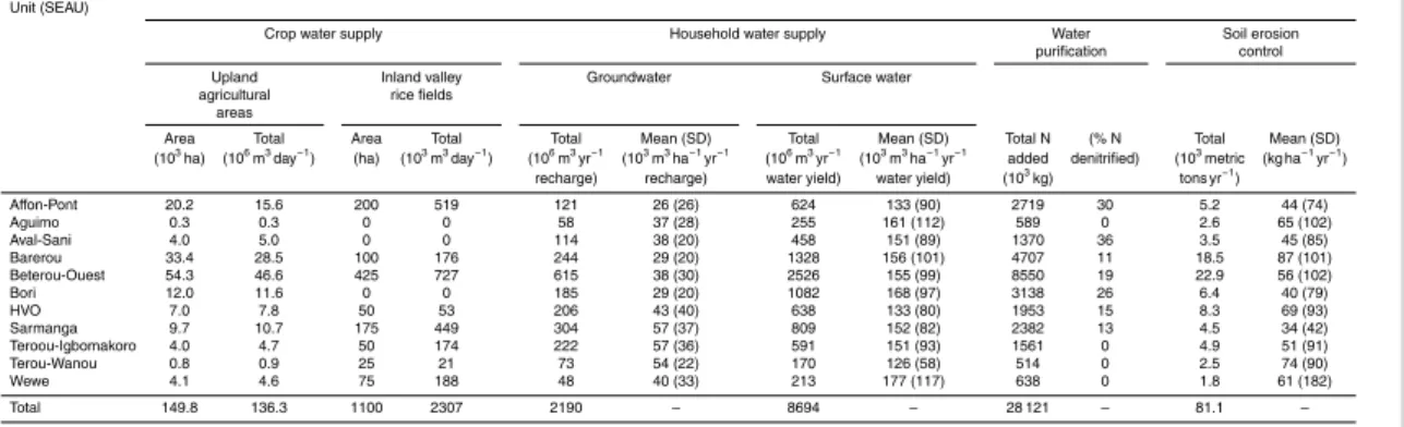
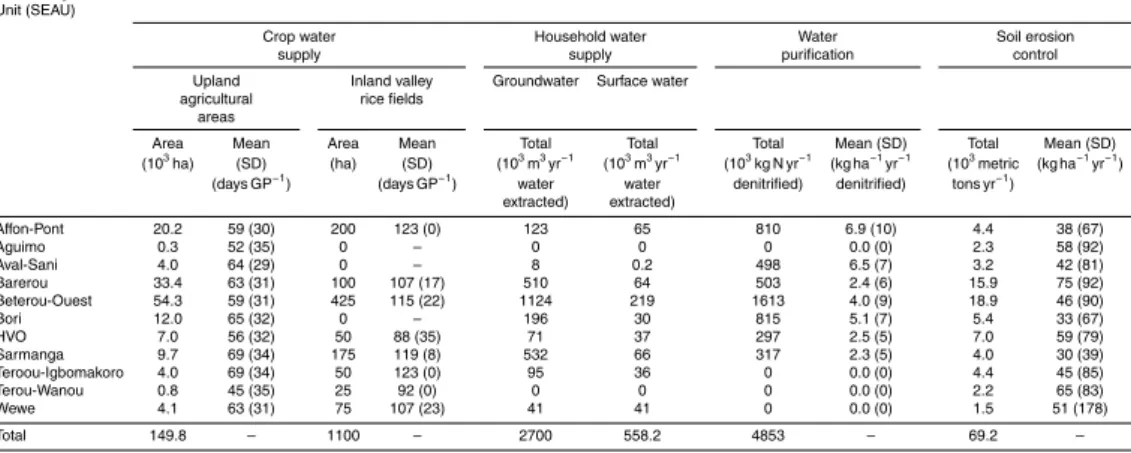
Biophysical ecosystem accounts are the basis for monetary accounting and were set up in accordance with SEEA-Experimental Ecosystem Accounting guidelines (EC et al., 2013). We defined eleven Subwatershed Ecosystem Accounting Units (SEAUs) which were then used to set up service capacity and service flow accounts. The SEAUs were defined based on the drainage areas of streamflow monitoring stations within 20
the watershed from a total of 44 subwatersheds. The monitoring stations are listed in Table 3. The 44 subwatersheds were delineated from the ASTER Global Digital Elevation Map as part of the initial model setup with ArcSWAT. Some monitoring stations with smaller drainage areas were nested within those with larger drainage areas. Because we wanted to set up spatially disaggregated accounts, in such cases 25
HESSD
12, 3477–3526, 2015Modelling ecosystem services for
ecosystem accounting
C. Duku et al.
Title Page
Abstract Introduction
Conclusions References
Tables Figures
◭ ◮
◭ ◮
Back Close
Full Screen / Esc
Printer-friendly Version Interactive Discussion
Discussion
P
a
per
|
Discussion
P
a
per
|
Discussion
P
a
per
|
Discussion
P
a
per
|
cell (500 m×500 m) and service flow-load per grid cell (500 m×500 m) that had been computed in Sect. 3.2 were then aggregated.
A key motivation for ecosystem accounting is to provide information for tracking changes in ecosystems and linking those changes to economic and other human activities (EC et al., 2013). Trend analysis statistical tests were conducted on the 5
total annual values (or total seasonal values for crop water supply) of service capacity accounts in each SEAU. Trend analysis determines if the changes in service capacity over time are due to random variability or statistically significant and consistent changes. This was conducted using the non-parametric Mann–Kendall test for trend. The Mann–Kendall test for trend statistically determines if there is a monotonic upward 10
or downward trend of a variable over time. A trend was detected if temporal variation in service capacity was statistically significant at 5 % significance level (P value<0.05). If a trend was detected, the Mann–Kendall statistic and Sen’s slope estimator were calculated. The Mann–Kendall statistic is a measure of the strength and direction of a trend, whereas Sen’s slope estimator is a measure of the magnitude of a trend. 15
4 Results
4.1 SWAT Landscape model calibration and validation results
The model simulated streamflow and transport processes satisfactorily. Table 3 shows the statistical results of the model calibration and validation. Moriasi et al. (2007) recommends the following for statistical evaluation of model simulation: NSE>0.50 20
and RSR<0.70, PBIAS within the range −25 to 25 for streamflow, −55 to 55 for sediment, and −70 to 70 for nutrients. For this study, the NSE>0.5 were achieved in at least nine out of eleven stations during calibration and validation. Of the four stations located upstream, three achieved NSE scores≥0.7 during calibration and validation, whereas of the seven stations downstream, six achieved NSE scores≥0.7 25
HESSD
12, 3477–3526, 2015Modelling ecosystem services for
ecosystem accounting
C. Duku et al.
Title Page
Abstract Introduction
Conclusions References
Tables Figures
◭ ◮
◭ ◮
Back Close
Full Screen / Esc
Printer-friendly Version Interactive Discussion
Discussion
P
a
per
|
Discussion
P
a
per
|
Discussion
P
a
per
|
Discussion
P
a
per
|
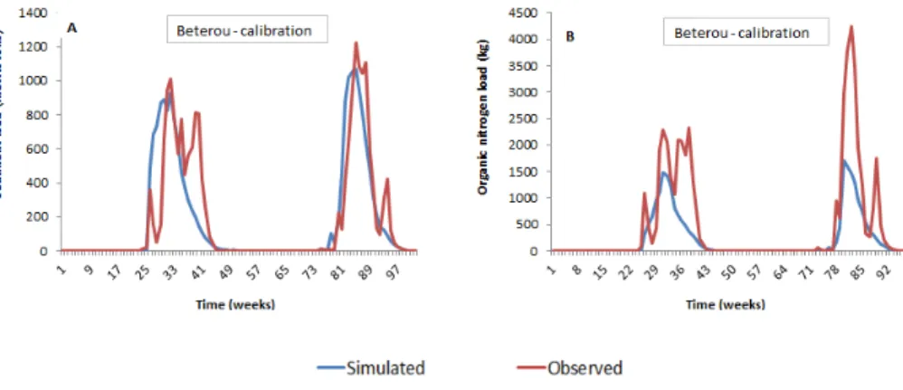
calibration and overestimated it during validation, however, PBIAS scores for at least seven stations were within the acceptable range. The RSR scores of a majority of the monitoring stations were also within the acceptable range. Overall, at different spatial scales, (e.g. Wewe, 297 km2; Igbo, 2309 km2; Beterou, 10 046 km2), the model simulated hydrological processes satisfactorily as is shown in Fig. 2. The graphical 5
results of sediment load and organic nitrogen load calibration are shown in Fig. 3. Similar to calibration of streamflow, the model underestimated sediment and organic nitrogen loads. The NSE, PBIAS and RSR scores shown in Table 3 were, however, satisfactory and within the acceptable range.
4.2 Spatial patterns of hydrological ecosystem services
10
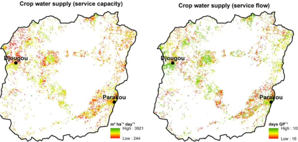
Water supply by soil moisture is essential to reduce crop water stress in rainfed agricultural systems. High service flow indicates low crop water stress. If all other factors for crop growth (such as nutrients, temperature) remain constant, then a higher service flow results in a higher crop yield. Crop water supply was spatially restricted to upland agricultural areas (with length of growing period of 103 days) and inland 15
valley rice fields (with length of growing period of 123 days). Figure 4 reveals high spatial variability in service capacity and service flow in upland agricultural areas. All upland agricultural areas were simulated with the same crop type, maize. As a result, the values of service flow should be interpreted as that of a spatial unit under maize cultivation. The spatial distribution of mean seasonal values of service capacity and 20
service flow in inland valley rice fields are not shown because of their significantly low total area (less than 1 % of total cropland area). Mean seasonal values of service capacity in inland valleys ranged from 577 to 3660 m3ha−1day−1 with a watershed-wide mean of 2086 m3ha−1day−1 and a SD of 1056 m3ha−1day−1. Mean seasonal values of service flow in inland valleys ranged from 67 to 123 days with a watershed-25
HESSD
12, 3477–3526, 2015Modelling ecosystem services for
ecosystem accounting
C. Duku et al.
Title Page
Abstract Introduction
Conclusions References
Tables Figures
◭ ◮
◭ ◮
Back Close
Full Screen / Esc
Printer-friendly Version Interactive Discussion
Discussion
P
a
per
|
Discussion
P
a
per
|
Discussion
P
a
per
|
Discussion
P
a
per
|
least 90 days whereas less than 25 % (approximately 36 000 ha) of upland agricultural areas recorded mean seasonal values of service flow of at least 90 days.
The spatial distribution of mean annual values of service capacity and service flow of groundwater supply and surface water supply are shown in Figs. 5 and 6 respectively. Groundwater is the major source of water for household consumption 5
(drinking and non-drinking purposes) with the service flow (groundwater extraction) significantly higher than service flow of surface water supply (surface water extraction). High service flows of groundwater supply are concentrated in the most populous towns in the watershed. However, service flows in Parakou, which is the most populous city in the watershed, are relatively lower than other areas such as Djougou. This is because 10
the population in Parakou depend mainly on tap water sources. Service capacity of groundwater supply exhibited high spatial variability. High values of service capacity were concentrated in the south-western part of the watershed. For service capacity of surface water supply, Fig. 6 shows areas with a high propensity for generating water yield. These areas, referred to as Hydrologically Sensitive Areas (HSAs) (Agnew et al., 15
2006), were not peculiar to a particular land cover type. They occurred in almost all land cover types. They occurred more frequently in savannah woodland and shrubland because approximately 80 % of the total watershed area is either one of this land cover type.
Water purification modelled as denitrification is essential to control the quantities of 20
nitrate available for leaching and contaminating groundwater resources (Jarvis, 2000; Jahangir et al., 2012). Service capacity was measured as the percentage of nitrate that is denitrified and service flow was the rate of denitrification. The spatial distribution of mean annual values of service capacity and service flow of water purification are distinctly concentrated in the northern and eastern parts of the watershed with 25
HESSD
12, 3477–3526, 2015Modelling ecosystem services for
ecosystem accounting
C. Duku et al.
Title Page
Abstract Introduction
Conclusions References
Tables Figures
◭ ◮
◭ ◮
Back Close
Full Screen / Esc
Printer-friendly Version Interactive Discussion
Discussion
P
a
per
|
Discussion
P
a
per
|
Discussion
P
a
per
|
Discussion
P
a
per
|
to take place. In areas where denitrification was recorded, the highest mean annual values of service flow were recorded in inland valley rice fields (12 kg ha−1yr−1) and grasslands (7 kg ha−1yr−1). The highest mean annual values of service capacity were also recorded in grasslands (55 % yr−1) and inland valley rice fields (35 % yr−1).
The spatial distributions of mean annual values of service capacity and service flow 5
of soil erosion control are shown in Fig. 8. High service capacity indicates high potential for soil erosion in the absence of vegetation cover. The sensitivity of a spatial unit to soil erosion in the absence of a specific vegetation cover type is a measure of the sediment retention potential of that vegetation cover type. The service flow, however, is a measure of the actual rate of sediment retention under prevailing vegetation 10
cover. Overall, soil erosion is currently not a problem in the watershed with a mean annual rate of sediment yield of 0.01 metric tons ha−1yr−1 (SD of 0.02 metric ton ha−1yr−1). However, the service capacity map reveals that soil erosion will increase significantly to a mean annual value of 0.05 metric tons ha−1yr−1 (SD of 0.07 metric ton ha−1yr−1) should there be loss of vegetation cover. Under existing vegetation cover 15
and management conditions, a mean annual sediment retention rate of 0.04 metric tons ha−1yr−1(SD of 0.07 metric ton ha−1yr−1) was recorded for service flow. For both service capacity and service flow, only about 0.04 % of the total area of the watershed recorded mean annual values greater than 1 metric ton ha−1yr−1. These areas had the steepest slopes, indicating the importance of vegetation cover in soil erosion control in 20
these areas. In forested areas, service flow was equal to service capacity, indicating that overall there was no net soil loss from forested areas.
4.3 Biophysical ecosystem accounts
The service capacity (Table 4) and service flow (Table 5) ecosystem accounting tables show the distribution of hydrological ecosystem services across the eleven 25
HESSD
12, 3477–3526, 2015Modelling ecosystem services for
ecosystem accounting
C. Duku et al.
Title Page
Abstract Introduction
Conclusions References
Tables Figures
◭ ◮
◭ ◮
Back Close
Full Screen / Esc
Printer-friendly Version Interactive Discussion
Discussion
P
a
per
|
Discussion
P
a
per
|
Discussion
P
a
per
|
Discussion
P
a
per
|
However, the mean values for service capacity varied depending on the biophysical environment of an SEAU. For example, whereas the Beterou-Ouest SEAU is the largest, the highest mean service capacity of groundwater supply was recorded in Sarmanga and Terou-Igbomakoro SEAUs. This signifies that the rate of groundwater recharge is highest in Sarmanga and Terou-Igbomakoro SEAUs. The service flow 5
table reveals that the ecohydrological conditions required for denitrification (water purification) do not occur in Aguimo, Terou-Igbomakoro, Terou-Wanou, and Wewe SEAUs. However, a total of 77 000 m3 of groundwater was extracted in Terou-Igbomakoro and Wewe SEAUs in 2012. In Aguimo and Terou-Wanou SEAUs, there is currently no groundwater extraction. For crop water supply, the tables also show the 10
total area of land currently under crop cultivation in each SEAU. Upland agricultural areas provide over 99 % of total cropland area. The SEAUs with the largest upland agricultural areas did not necessarily record the highest service flow. For example, the highest service flow was recorded in Sarmanga and Terou-Igbomakoro. This signifies that maize cultivation in these SEAUs is less prone to water stress than in any other 15
SEAUs.
Temporal analysis of ecosystem accounts makes it possible to track ecosystem changes and measure the degree of sustainability, degradation or resilience. Decreasing capacity of ecosystems to sustain human welfare over time is a measure of ecosystem degradation (EC et al., 2013). Figure 9 shows the results of trend 20
analysis statistical tests of service capacities at the SEAU level. Decreasing trends were observed in crop water supply (in upland agricultural areas) in all the SEAUs except Terou-Igbomakoro. In the Terou-Igbomakoro SEAU there was no trend observed in service capacity of crop water supply. The results shown in Fig. 9a are of the five SEAUs that recorded the highest slope as measured with the Mann–Kendall statistic. 25
HESSD
12, 3477–3526, 2015Modelling ecosystem services for
ecosystem accounting
C. Duku et al.
Title Page
Abstract Introduction
Conclusions References
Tables Figures
◭ ◮
◭ ◮
Back Close
Full Screen / Esc
Printer-friendly Version Interactive Discussion
Discussion
P
a
per
|
Discussion
P
a
per
|
Discussion
P
a
per
|
Discussion
P
a
per
|
and surface water supply. For ground water supply, increasing trends were observed in all SEAUs. The results in Fig. 9c are of the five SEAUs with the highest Mann– Kendall statistic. Increasing trend of surface water supply was observed in four SEAUs, whereas increasing trend of water purification was observed in only the Aval-Sani SEAU. No statistically significant trend was observed in service capacity of soil erosion 5
control in all the SEAUs.
5 Discussion
In this section, we will discuss some of the broader lessons learnt from setting up biophysical ecosystem accounts for hydrological ecosystem services in the Upper Ouémé watershed. We will also discuss some of the implications for watershed and 10
ecosystem management.
5.1 Lessons for ecosystem accounting
In this study, we have shown how ecohydrological modelling can support ecosystem accounting. Setting up spatially disaggregated ecosystem accounts allows for the analysis of flow of services between regions, households, businesses, income groups 15
etc. (EC et al., 2013). There has been a variety of approaches to model hydrological ecosystem services. However, our approach allows for the organisation and analysis of biophysical data on hydrological ecosystem service capacity and service flow at different spatial and temporal scales suitable for the development, monitoring and evaluation of public policy.
20
HESSD
12, 3477–3526, 2015Modelling ecosystem services for
ecosystem accounting
C. Duku et al.
Title Page
Abstract Introduction
Conclusions References
Tables Figures
◭ ◮
◭ ◮
Back Close
Full Screen / Esc
Printer-friendly Version Interactive Discussion
Discussion
P
a
per
|
Discussion
P
a
per
|
Discussion
P
a
per
|
Discussion
P
a
per
|
administrative areas. Ecosystem accounting is normally applied at large spatial scales in order to upscale the results to a national level (EC et al., 2013). In such situations, it is important for operational feasibility of a model to strike a balance between spatial explicitness and computational efficiency. For the SWAT Landscape model (and SWAT model), increasing spatial detail results in a considerable increase in 5
computing time, irrespective of the spatial discretization scheme employed (Arnold et al., 2010; Notter et al., 2012). In our case-study area, over 1 400 000 grid cells are generated at 1 ha resolution requiring over two days for each simulated year on 2.6 GHz and 8 GB RAM. We acknowledge that in many regions of the world high-resolution spatial input data may not be available at large spatial scales. However, for 10
the grid-based setup of the SWAT Landscape model, when such high-resolution spatial data are available, it may be necessary to compromise spatial explicitness to achieve operational feasibility. Such decisions should be made taking into consideration the degree of spatial heterogeneity of landscape features (such as land cover and land use, soil and topography). Furthermore, it is important to follow this up with robust spatial 15
calibration and validation at different scales. Long-term time series data from a wide network of monitoring stations within a watershed needed for such spatial calibration and validation, however, may not always be available.
In ecosystem accounting, detailed and accurate land cover and land use data are important. Apart from their use as inputs in modelling ecosystem services, land cover 20
classes are also used as ecosystem accounting units based on which ecosystem services are aggregated (e.g. Remme et al., 2014; Schröter et al., 2014). A single lumped land cover class for agricultural areas or croplands (be it as model input data or ecosystem accounting units) may be suitable when modelling and accounting for other ecosystem services (e.g. Remme et al., 2014; Schröter et al., 2014). However, 25
HESSD
12, 3477–3526, 2015Modelling ecosystem services for
ecosystem accounting
C. Duku et al.
Title Page
Abstract Introduction
Conclusions References
Tables Figures
◭ ◮
◭ ◮
Back Close
Full Screen / Esc
Printer-friendly Version Interactive Discussion
Discussion
P
a
per
|
Discussion
P
a
per
|
Discussion
P
a
per
|
Discussion
P
a
per
|
is the major limitation to crop production and is the main factor responsible for low yields in the seasonally dry and semiarid tropics and subtropics (Shaxson and Barber, 2003). However, in many of these regions, land cover and land use data with this level of detail are currently not available. Obtaining such information is complicated by the small plot sizes and cropping patterns varying from year to year. Our study area was 5
no exception. Despite these constraints, the lack of detailed data reduces the accuracy and reliability of modelled results of service flow of crop water supply. In our study area, this limitation resulted in the simulation of only a single crop type in upland agricultural areas. Therefore, the results for service flow of crop water supply should be interpreted in the context of the crop simulated. However, because methodologies such as Allen 10
et al. (1998) have been used extensively to compute the water requirements of various crops, our approach serves as a reference or baseline from which the service flow of crop water supply of a spatial unit could be estimated if a crop other than maize is grown.
A key feature of ecosystem accounting is the distinction between service capacity 15
and service flow. The empirical distinction and separate spatial characterisation of service capacity and service flow is essential in understanding the dynamics of service provision and in planning and devising sustainable management options. The distinction is also important for subsequent monetary valuation. Service capacity and service flow should be based on measurable indicators that have policy and 20
management relevance. Indicators must also be able to represent cause–effect relations. For hydrological ecosystem services, selecting single indicators of service capacity that meet the above requirements and that sufficiently reflect ecosystem condition and their potential to provide service flows is difficult. This is because of the non-linear complex interactions among several ecohydrological processes that each 25
HESSD
12, 3477–3526, 2015Modelling ecosystem services for
ecosystem accounting
C. Duku et al.
Title Page
Abstract Introduction
Conclusions References
Tables Figures
◭ ◮
◭ ◮
Back Close
Full Screen / Esc
Printer-friendly Version Interactive Discussion
Discussion
P
a
per
|
Discussion
P
a
per
|
Discussion
P
a
per
|
Discussion
P
a
per
|
yields are related to inadequate soil moisture rather than to erratic rainfall because crop and land management do not optimise water flow along the rooting zone of the crop (Shaxson and Barber, 2003). Furthermore, Ennaanay (2006) and Yan et al. (2013) reported that changes in land use and other ecosystem components alter the hydrological cycle, affecting patterns of evapotranspiration, infiltration, water retention, 5
groundwater recharge and water yield. However, for services such as water purification and soil erosion control, the capacity indicators presented in this study are derived indicators and not actual physical processes. Such indicators do not convey information regarding key physical processes and therefore may not have management relevance. In such cases, a key question that arises is if the underlying ecosystem components 10
and processes should be weighted and aggregated to produce one composite indicator for service capacity (Edens and Hein, 2013). For example, soil erosion control is a function of surface runoff, slope, soil erodibility, cover and management factors, and support practice factors. Weighing and aggregation of ecosystem components and processes to establish a composite indicator for service capacity, however, is not 15
straightforward and is challenging (e.g. Weber, 2007; Stoneham et al., 2012).
5.2 Implications for watershed and ecosystem management
Three of the key issues critical for watershed management and land use planning in an agricultural watershed such as the Upper Ouémé are nitrate leaching, non-point source pollution and alteration in streamflow regime. Nitrate leaching contaminates 20
groundwater resources (Jahangir et al., 2012; Jarvis, 2000). Agricultural non-point source pollution leads to pollution of river networks (Agnew et al., 2006). Alteration of streamflow regime affects riverine ecological integrity and downstream water availability (Carlisle et al., 2011). Ecosystem accounting and spatial characterization of hydrological ecosystem services capacity and flow provide relevant information 25
HESSD
12, 3477–3526, 2015Modelling ecosystem services for
ecosystem accounting
C. Duku et al.
Title Page
Abstract Introduction
Conclusions References
Tables Figures
◭ ◮
◭ ◮
Back Close
Full Screen / Esc
Printer-friendly Version Interactive Discussion
Discussion
P
a
per
|
Discussion
P
a
per
|
Discussion
P
a
per
|
Discussion
P
a
per
|
watershed ecohydrology) or high service production areas (i.e., areas that are crucial for maintaining water flow downstream).
For example, our analyses reveal areas where the ecohydrological conditions required for denitrification do not occur but where there is currently groundwater extraction. These areas are high-risk areas of groundwater contamination from nitrate 5
leaching. More crucially, there is currently crop cultivation in some of these areas. Agricultural intensification in these areas, therefore, will result in higher nitrate leaching and contamination of groundwater resources.
Furthermore, the grid-based setup of the SWAT Landscape model enabled us to identify Hydrologically Sensitive Areas (HSAs) at a finer spatial resolution. 10
Characterization of the spatiotemporal dynamics of HSAs is essential in controlling non-point source pollution and in maintaining streamflow regime. Hydrologically Sensitive Areas have significant impact on key ecohydrological processes affecting interaction and transport of water, sediment, nutrients and pollutants. They also provide key landscape controls on riverine ecosystem integrity including aquatic flora and fauna 15
and downstream water availability and quality. Agricultural intensification in HSAs has a higher potential of generating agricultural non-point source pollution (Agnew et al., 2006). Land use change in these areas can have a more significant impact on the streamflow regime.
Such analyses can form the basis for establishing Payment for Ecosystem Services 20
schemes (Pagiola and Platais, 2007; Turpie et al., 2008). Watershed PES provide financial support to ecosystem management in high service production areas that are of particular relevance downstream (e.g. Lopa et al., 2012; Lu and He, 2014). We acknowledge that detailed ecohydrological modelling is only one of the considerations in establishing a watershed PES. Other considerations include transaction costs and 25
HESSD
12, 3477–3526, 2015Modelling ecosystem services for
ecosystem accounting
C. Duku et al.
Title Page
Abstract Introduction
Conclusions References
Tables Figures
◭ ◮
◭ ◮
Back Close
Full Screen / Esc
Printer-friendly Version Interactive Discussion
Discussion
P
a
per
|
Discussion
P
a
per
|
Discussion
P
a
per
|
Discussion
P
a
per
|
In this study, we also detected trends in changes in the capacity of watershed ecosystems to provide service flows. Detection of trends in service capacity is the first step towards measuring degradation or resilience. To determine the causes of these changes in service capacity will require further analysis such as detailed correlation analysis between each hydrological ecosystem service and the suite of underlying 5
ecohydrological processes. This was, however, beyond the scope of this study.
6 Conclusion
There are various components involved in ecosystem service delivery that need to be measured in order to better understand the full dynamics of service provision and to devise sustainable management options. Key amongst these components 10
are service capacity and service flow. Empirical distinction of service capacity and service flow of ecosystem services is a distinguishing feature of ecosystem accounting. Our analyses show that integrating hydrological ecosystem services in an ecosystem accounting framework provides relevant information on watershed ecosystems and hydrological ecosystem services at appropriate scales suitable for decision-making. 15
They show that for watershed management, land use planning and land management, measurement of service flow should go hand in hand with managing service capacity. For hydrological ecosystem services in which high service capacity areas and high service flow areas are not spatially coincident, such empirical distinction and separate spatial characterization are much more crucial. Ecohydrological modelling to support 20
ecosystem accounting, therefore, requires appropriate decisions regarding model process inclusion, physical and mathematical representation, spatial heterogeneity, temporal resolution, and model accuracy.
We have shown that despite the non-linear complex interactions among several ecohydrological processes that each relies on a suite of ecosystem components; 25
HESSD
12, 3477–3526, 2015Modelling ecosystem services for
ecosystem accounting
C. Duku et al.
Title Page
Abstract Introduction
Conclusions References
Tables Figures
◭ ◮
◭ ◮
Back Close
Full Screen / Esc
Printer-friendly Version Interactive Discussion
Discussion
P
a
per
|
Discussion
P
a
per
|
Discussion
P
a
per
|
Discussion
P
a
per
|
in time and space of ecosystems to productive and consumptive human activities leading to human benefits, whereas the service capacities we modelled reflect ecosystem condition and extent at a point in time, and the resulting potential to provide service flows. We demonstrated our approach by using a grid-based setup of a modified SWAT model, SWAT Landscape, to map and quantify four hydrological 5
ecosystem services vital to human well-being in the Upper Ouémé watershed. We set up ecosystem accounting tables for both service capacity and service flow and analysed trends in service capacities. For each hydrological ecosystem service, we were able to identify Subwatershed Ecosystem Accounting Units (SEAUs) where either service capacity or service flow is concentrated. We were also able to identify trends 10
in changes in service capacity of hydrological ecosystem services for some SEAUs. Our approach can be extended and applied to other watersheds because it is based on the robust SWAT model, which has been tested extensively in different watersheds and landscapes.
Author contributions. C. Duku, L. Hein and S. J. Zwart conceived and designed the study;
15
H. Rathjens developed the grid-based model code; C. Duku performed the simulations and analyses; C. Duku and L. Hein prepared the manuscript with contributions from S. J. Zwart and H. Rathjens.
Acknowledgements. This research was conducted at Wageningen University as part of the project “Realizing the potential of inland valley lowlands in sub-Saharan Africa while maintaining
20
their environmental services” (RAP-IV). The project is implemented by the Africa Rice Center and its national partners and is funded by the European Commission through the International Fund for Agricultural Development (IFAD). We thank the IMPETUS project in Benin for making data available for this research through their public geoportal. We are grateful to Christophe Peugeot and the AMMA-CATCH regional observing system in Benin for providing
25
HESSD
12, 3477–3526, 2015Modelling ecosystem services for
ecosystem accounting
C. Duku et al.
Title Page
Abstract Introduction
Conclusions References
Tables Figures
◭ ◮
◭ ◮
Back Close
Full Screen / Esc
Printer-friendly Version Interactive Discussion
Discussion
P
a
per
|
Discussion
P
a
per
|
Discussion
P
a
per
|
Discussion
P
a
per
|
References
Abbaspour, K., Yang, J., Reichert, P., Vejdani, M., Haghighat, S., and Srinivasan, R.: SWAT-CUP, SWAT Calibration and Uncertainty Programs, Swiss Federal Institute of Aquatic Science and Technology (EAWAG), Zurich, Switzerland, 2008.
Agnew, L. J., Lyon, S. W., Gerard-Marchant, P., Collins, V. B., Lembo, A. J., Steenhuis, T. S., and
5
Walter, M. T.: Identifying hydrologically sensitive areas: bridging the gap between science and application, J. Environ. Manage., 78, 63–76, doi:10.1016/j.jenvman.2005.04.021, 2006. Allen, R. G., Pereira, S. L., Raes, D., and Smith, M.: Irrigation and Drainage Paper 56, FAO,
Rome, Italy, 1998.
AMMA-CATCH Database: available at: http://bd.amma-catch.org/amma-catch2/main.jsf (last
10
access: 28 May 2014), 2014.
Arnold, J. G., Srinivasan, R., Muttiah, R. S., and Williams, J. R.: Large area hydrologic modeling and assessment – Part I: Model development, J. Am. Water Resour. As., 34, 73–89, 1998. Arnold, J. G., Muttiah, R. S., Srinivasan, R., and Allen, P. M.: Regional estimation of base
flow and groundwater recharge in the Upper Mississippi river basin, J. Hydrol., 227, 21–40,
15
doi:10.1016/S0022-1694(99)00139-0, 2000.
Arnold, J. G., Allen, P. M., Volk, M., Williams, J. R., and Bosch, D. D.: Assessment of different representations of spatial variability on swat model performance, T. ASABE, 53, 1433–1443, 2010.
Arnold, J. G., Kiniry, J. R., Srinivasan, R., Williams, J. R., Haney, E. B., and Neitsch, S. L.:
20
Soil Water and Assessment Tool Input/Output Documentation Version 2012, Texas Water Resources Institute, College Station, Texas, USA, 2013.
Bosch, D. D., Arnold, J. G., Volk, M., and Allen, P. M.: Simulation of a low-gradient coastal plain watershed using the swat landscape model, T. ASABE, 53, 1445–1456, 2010.
Boyd, J. and Banzhaf, S.: What are ecosystem services? The need for standardized
envi-25
ronmental accounting units, Ecol. Econ., 63, 616–626, doi:10.1016/j.ecolecon.2007.01.002, 2007.
Boyer, E. W., Alexander, R. B., Parton, W. J., Li, C. S., Butterbach-Bahl, K., Donner, S. D., Skaggs, R. W., and Del Gross, S. J.: Modeling denitrification in terrestrial and aquatic ecosystems at regional scales, Ecol. Appl., 16, 2123–2142,
doi:10.1890/1051-30