Modelos de Mapas Simpléticos para o
Movimento de Deriva Elétrica com Efeitos de
Raio de Larmor Finito
Júlio César David da Fonseca
Orientador: Prof. Dr. Iberê Luiz Cadas
Tese de doutorado apresentada ao Instituto de Física para a obtenção do título de Doutor em Ciências
Banca Examinadora:
Prof. Dr. Iberê Luiz Cadas (USP)
Prof. Dr. Edson Denis Leonel (UNESP - Rio Claro)
Prof. Dr. Ricardo Egydio de Carvalho (UNESP - Rio Claro) Prof. Dr. Ricardo Luis Viana (UFPR)
Prof. Dr. Roberto Venegeroles Nascimento (UFABC)
do Instituto de Física da Universidade de São Paulo
Fonseca, Júlio César David da
Modelos de mapas simpléticos para o movimento de deriva elétrica com efeitos de raio de Larmor finito. São Paulo, 2016.
Tese (Doutorado) – Universidade de São Paulo. Instituto de Física Depto. de Física Aplicada.
Orientador: Prof. Dr. Iberê Luiz Caldas
Área de Concentração: Física
Unitermos: 1. Física de plasmas; 2. Fenômeno de transporte; 3. Caos (Sistemas dinâmicos).
Area-Preserving Maps Models of the Electric
Drift Motion with Finite Larmor Radius
Effects
Júlio César David da Fonseca
Advisor: Prof. Dr. Iberê Luiz Cadas
Submitted to the Institute of Physics in partial fulfillment of the requirements for the degree of Doctor in Science.
Evaluation comitte:
Prof. Dr. Iberê Luiz Cadas (USP)
Prof. Dr. Edson Denis Leonel (UNESP - Rio Claro)
Prof. Dr. Ricardo Egydio de Carvalho (UNESP - Rio Claro) Prof. Dr. Ricardo Luis Viana (UFPR)
Prof. Dr. Roberto Venegeroles Nascimento (UFABC)
I would like to express my thanks to my thesis advisor Prof. Iberˆe L. Caldas for his
guidance.
I wish also to thank Dr. Diego del Castillo Negrete from the Oak Ridge National
Laboratory (USA), Prof. Igor M. Sokolov from Humboldt University in Berlin (Germany),
and Prof. Roberto Venegeroles from Federal University of ABC (Brazil) for their valuable
suggestions.
This work was supported by the brazilian research agencies CNPq and FAPESP.
Mapas simpl´eticos tˆem sido amplamente utilizados para modelar o transporte ca´otico
em plasmas e fluidos. Neste trabalho, propomos trˆes tipos de mapas simpl´eticos que
descrevem o movimento de deriva el´etrica em plasmas magnetizados. Efeitos de raio de
Larmor finito s˜ao inclu´ıdos em cada um dos mapas. No limite do raio de Larmor tendendo
a zero, o mapa com frequˆencia monotˆonica se reduz ao mapa de Chirikov-Taylor, e, nos
casos com frequˆencia n˜ao-monotˆonica, os mapas se reduzem ao mapa padr˜ao n˜ao-twist.
Mostramos como o raio de Larmor finito pode levar `a supress˜ao de caos, modificar a
topologia do espa¸co de fases e a robustez de barreiras de transporte. Um m´etodo baseado
na contagem dos tempos de recorrˆencia ´e proposto para analisar a influˆencia do raio de
Larmor sobre os parˆametros cr´ıticos que definem a quebra de barreiras de transporte.
Tamb´em estudamos um modelo para um sistema de part´ıculas onde a deriva el´etrica ´e
de-scrita pelo mapa de frequˆencia monotˆonica, e o raio de Larmor ´e uma vari´avel aleat´oria que
assume valores espec´ıficos para cada part´ıcula do sistema. A fun¸c˜ao densidade de
proba-bilidade para o raio de Larmor ´e obtida a partir da distribui¸c˜ao de Maxwell-Boltzmann,
que caracteriza plasmas na condi¸c˜ao de equil´ıbrio t´ermico. Um importante parˆametro
neste modelo ´e a vari´avel aleat´oria gama, definida pelo valor da fun¸c˜ao de Bessel de
or-dem zero avaliada no raio de Larmor da part´ıcula. Resultados anal´ıticos e num´ericos
descrevendo as principais propriedades estat´ısticas do parˆametro gama s˜ao apresentados.
Tais resultados s˜ao ent˜ao aplicados no estudo de duas medidas de transporte: a taxa de
escape e a taxa de aprisionamento por ilhas de per´ıodo um.
Area-preserving maps have been extensively used to model chaotic transport in
plas-mas and fluids. In this work we propose three types of maps describing electric drift motion
in magnetized plasmas. Finite Larmor radius effects are included in all maps. In the limit
of zero Larmor radius, the monotonic frequency map reduces to the Chirikov-Taylor map,
and, in cases with non-monotonic frequencies, the maps reduce to the standard nontwist
map. We show how the finite Larmor radius can lead to chaos suppression, modify the
phase space topology and the robustness of transport barriers. A method based on
count-ing the number of recurrence times is used to quantify the dependence on the Larmor
radius of the threshold for the breakup of transport barriers. We also study a model
for a system of particles where the electric drift is described by the monotonic frequency
map, and the Larmor radius is a random variable that takes a specific value for each
particle of the system. The Larmor radius’ probability density function is obtained from
the Maxwell-Boltzmann distribution, which characterizes plasmas in thermal equilibrium.
An important parameter in this model is the random variable gamma, defined by the
zero-order Bessel function evaluated at the Larmor radius’particle. We show analytical
and numerical computations related to the statistics of gamma. The set of analytical
results obtained here is then applied to the study of two numerical transport measures:
the escape rate and the rate of trapping by period-one islands.
1 Introduction 1
2 Gyro-Averaged E×B Maps and FLR Effects 7
2.1 Gyro-averaged E~ ×B~ Drift Model . . . 7
2.2 Gyro-averaged standard map (GSM) . . . 9
2.3 Gyro-averaged standard nontwist map (GSNM) . . . 12
2.3.1 Fixed Points . . . 14
2.3.2 Separatrix reconnection . . . 15
2.3.3 Nontwist transport barrier . . . 19
2.3.4 Breakup Diagrams . . . 20
2.4 Gyro-averaged quartic nontwist map (GQNM) . . . 29
2.4.1 Fixed Points and nontwist transport barriers . . . 31
2.4.2 Robustness of the central shearless curve . . . 33
3 Statistical Properties of the GSM Model 39 3.1 GSM Model . . . 39
3.1.1 Maxwell-Boltzmann Distribution . . . 40
3.1.2 Larmor Radius’ PDF . . . 41
3.2 Gamma’s Probability Density Function . . . 43
3.3 Gamma’s Average and Dispersion . . . 47
3.4 Gamma’s Cumulative Distribution Function . . . 49
3.5 Probability of Global Chaos (Pc) . . . 53
3.6 Escape Rate . . . 56
3.7 Rate of Trapping by Period-One Islands . . . 60
4 Conclusion 69 Appendices 75 A Gyro-averaged Drift Wave Map 77 B Indicator Points 81 B.1 GSNM Indicator Points . . . 81
B.1.1 Involutions and Symmetry . . . 81
B.1.2 Fixed Points of SI0 and SI1 . . . 83
B.2 GQNM Indicator Points . . . 85
C Statistics of Gamma: Further Results 87 C.1 Alternative form of the Gamma’s PDF . . . 87
C.2 Moments . . . 94
Introduction
Important research efforts in controlled nuclear fusion are focused on the magnetic
confinement of hot plasmas. In order to improve the confinement conditions, a better
understanding of the particle transport is needed, specially in the case of electric drift
motion or, simply, E~ ×B~ transport. A typical approach to this problem is based on the
~
E ×B~ approximation of charged particle’s guiding center’s motion [1–4]. However, in case of fast particles (e.g. alpha particles in burning plasmas) or inhomogeneous fields
on the scale of the Larmor radius, it is necessary to consider finite Larmor radius (FLR)
effects [5, 6].
Previous studies on the role of the Larmor radius include Refs. [5, 7, 8], where
non-diffusive particle transport in numerical simulations of eletrostatic turbulence was
ana-lyzed and FLR effects were shown to inhibit transport. Non-diffusive chaotic transport
was studied in [9] using an E~ × B~ Hamiltonian model that incorporates FLR effects. In [6, 10], the authors studied another Hamiltonian model of the E~ ×B~ transport with FLR effects, making use of dynamical systems methods to investigate Larmor radius’s
influence on the formation of complex phase space topologies and chaos supression.
In this work we analyse FLR effects in simple area preserving maps models of E~ ×B~
motion. The maps presented here are constructed following the Hamiltonian framework
in [11] for electrostatic drift motion. The Hamiltonian is determined by a time dependent
electrostatic potential, which depends on the radial and the poloidal coordinates. FLR
corrections are included into the model by gyro-averaging [12] the electrostatic potential.
The electrostatic potential consists of two parts: the first one depends only on the
radial coordinate and is called the equilibrium potential; the second part, which depends
on time and the poloidal coordinate, represents a superposition of drift waves. We model
the drift waves following the approach in [13] that allows the contruction of area
preserv-ing maps as simple discrete models of E~ ×B~ transport. Depending on the equilibrium potential, the maps’ frequencies exhibit monotonic or non-monotonic profiles. Using these
simple maps models of gyro-averaged chaoticE~×B~ transport, we analyze the role of Lar-mor radius in the following problems: chaos supression, stability of fixed points, nontwist
phase space topologies, and transport barriers.
The term “nontwist” is used to designate Hamiltonian systems that violate the twist
or nondenegeracy property. That is the case for Hamiltonian systems whose frequency
is a non-monotonic function of the action variable. Nontwist Hamiltonian systems are
characterized by particular phase space topologies [14] and can be found in many different
physical models. Some examples include: E×B transport in magnetized plasmas [3, 4, 15]; magnetic fields with reverse shear in toroidal plasma devices [16–18]; modelling of
transport by traveling waves in shear flows in fluids [19–21].
The presence of nontwist transport barriers is among the most important properties
exhibited by nontwist Hamiltonian systems. By nontwist transport barriers we mean a
robust region of spanning Kolmogorov-Arnold-Moser (KAM) curves that are resistant to
“breakup”, i.e. they can survive even when the phase space is almost completely dominated
by chaotic dynamics. In Hamiltonian dynamical systems theory, spanning KAM curves,
also called KAM barriers [19] or rotational invariant circles [22], are known to divide
the phase space in such a way that chaotic orbits become confined among them. For this
reason, spanning KAM curves are interesting in the study of transport problems, specially
those related to E×B Hamiltonian models. In the context of one and a half degrees of freedom nontwist Hamiltonian systems, the robusteness of spanning KAM curves has also
been called strong KAM stability [23] and has been the subject of several studies (see, for
example, [24–27] and references therein).
In this work the maps correspond to Hamiltonians whose frequencies can be monotonic
presence of nontwist transport barriers that can be destroyed or restored by changing the
value of the Larmor radius. This feature is directly related to the FLR effect of chaotic
transport suppression, whose study was initiated by [6, 10]. Here we show that chaos
suppression occurs when the Larmor radii are close to specific values, for which invariant
circles become very resilient to breakup. In the case of the nontwist maps, the invariant
circles that constitute the nontwist transport barrier are the most easily restored and
hardest to break.
Among the main goals of the present work is the study of the critical parameters related
to the destruction of nontwist barriers. These thresholds can be aproximately determined
by what we call here the breakup diagrams. In order to efficiently compute breakup
diagrams, this work describes a procedure based on a technique [28] which explores the
recurrence properties of a dynamical system’s orbit that result from the Slater’s Theorem
[29]. As shown in [28], and also in the later work [30], the recurrence properties of an
orbit can be used to differentiate chaotic and non-chaotic motion. A recent example of
the application of this technique to the standard nontwist map [19] was presented in [31].
We also study statistical properties of a model based on the gyro-averaged standard map (GSM), the simplest area-preserving map proposed in this this work. The GSM corresponds to the map with monotonic frequency map and is a modified version of the
Chirikov-Taylor or standard map [32, 33].
Besides a perturbation parameter, the GSM has a dependence on a function gamma,
given by the zero-order Bessel function of the Larmor radius. The GSM’seffective pertur-bation consists in the product between the perturbation parameter and gamma. In the limit of zero Larmor radius, the GSM corresponds exactly to the standard map.
In the GSM model initially analyzed, we have assumed the Larmor radius as a
param-eter and our goal was to study non-linear dynamics properties emerging from changing
the value of this parameter. After concluding this study, we adapted the GSM model
in order to consider an ensemble of charged particles, each one having its own Lamor
radius. Following [6,9], the Larmor radius’ probability density function (pdf) results from
a Maxwell-Boltzmann distribution, which describes plasmas in thermal equilibrium.
different GSMs, each one with its own effective perturbation. Thus, particles“see”different
phase space topologies: a particle can be trapped inside an stability island as other one,
after crossing the orbit of the first, is able to reach far regions of the phase space following
chaotic orbit.
Since the effective perturbation depends on the value of gamma, determining its basic
statistical features is important to any transport study in the GSM model. Using the
Larmor radius’ pdf, we start by obtaining a set of analytical expressions including the
pdf, the average and the dispersion of gamma. Histograms of gamma are discussed using
the formulas obtained.
An analytical formula for the cumulative distribution function of gamma is also
pre-sented and verified by numerical simulations. We describe its main properties and relate
them to the gamma’s pdf. The cumulative distribution function of gamma is then
ap-plied to obtain two additional analytical results: the probability of global chaos and the
probability of trapping by period-one islands.
The probability of global chaos is the probability of a particle moving in a phase
space characterized by global chaos, i.e. a phase space where KAM barriers do not exist.
The probability of trapping by period-one islands is the probability of a particle, initially
located near a fixed point, being trapped by the corresponding period-one island. If the
fixed point is elliptic, there is an island trapping particles near it. In case of an hyperbolic
fixed point, particles, in general, move away from it following chaotic orbits.
The probabilities of global chaos and trapping are functions depending on the thermal
Larmor radius and the perturbation parameter, the only two parameters in GSM model
and that incorporate all relevant physics. We show plots of both probabilities, analyzing
how they change regarding variations of the two parameters.
To illustrate the application of the analytical results obtained, we define and analyze
two numerical transport measures: the escape rate and the rate of trapping by
period-one-islands. Numerical simulations of both measures are shown and compared to the
probabilites of global chaos and trapping. The role of the thermal Larmor radius and the
perturbation parameter is again analyzed in detail.
In chapter 2, we introduce a discrete model of the gyro-averaged E~ ×B~ drift motion, which we call here as gyro-averaged drift wave map. The model is used to construct all
maps discussed in this work. Non-linar dynamics properties resulting from FLR effects
are studied for each of those maps.
In chapter 3, we focus on the statistical analysis of the GSM model.
In chapter 4, we present a summary and concluding remarks.
Appendix A describes the details in the obtention of the gyro-averaged drift wave map.
Appendix B shows necessary conditions and computations to obtain indicator point
formulas, which are important to detect the presence of nontwist transport barriers.
In the last chapter, Appendix C, we present an alternative approach to obtain the main
Gyro-Averaged E
×
B Maps and
FLR Effects
This chapter is organized as follows. Section 2.1 describes the discrete model of
gyro-averaged E~ ×B~ drift motion, from which we derive different kinds of maps. The first example, for which the frequency has a monotonic profile, is presented in section 2.2,
where FLR effects on the transition to global chaos are analyzed. Section 2.3 describes an
example with a non-monotonic profile and dicusses FLR effects on the stability of fixed
points, phase space topologies and breakup diagrams. Another nontwist map is analysed
in section 2.4, where we turn our attention to FLR effects on zonal flow bifurcations. This
chapter is partly based on Ref. [34], our last published paper.
2.1
Gyro-averaged
E
~
×
B
~
Drift Model
The E~ ×B~ drift velocity of the guiding center is given by [35]:
~vGC =
~ E×B~
B2 . (2.1)
Using x as the radial coordinate and y as the poloidal coordinate, the equations of the
~
E×B~ drift motion, given by~vGC = ( ˙x(t),y˙(t)), can be written as the Hamiltonian system:
dy dt =
∂H(x, y, t)
∂x ,
dx dt =−
∂H(x, y, t)
∂y , (2.2)
where:
H(x, y, t) = φ(x, y, t)
B0
, (2.3)
φis the electrostatic potential, and we assume a constant toroidal magnetic fieldB~ =B0eˆz.
As discussed in [10], finite Larmor radius (FLR) effects can be incorporated substituting
the electrostatic potential by its average over a circle around the guiding center:
hφ(x, y, t)iϕ =
1 2π
Z 2π
0
φ(x+ρcosϕ, y+ρsinϕ, t)dϕ, (2.4)
where ρ is the Larmor radius, which defines the radius of a charged particle’s gyration around its guiding center, and the integration variableϕis the angle of gyration. Formula
(2.4) corresponds to the well-known gyro-averaging operation [12]. The gyro-averaged Hamiltonian can then be defined as:
hH(x, y, t)iϕ = h
φ(x, y, t)iϕ
B0
, (2.5)
and the gyro-averaged equations of motion (2.2) can be written as:
dy dt =
∂hHiϕ
∂x ,
dx dt =−
∂hHiϕ
∂y . (2.6)
Following [13], we assume an electrostatic potential of the form:
φ(x, y, t) = φ0(x) +A +∞
X
m=−∞
cos(ky−mω0t), (2.7)
where φ0(x) is the equilibrium potential, A, the amplitude of the drift waves, k is the
wave number, andω0 is the fundamental frequency.
Applying the gyro-average operation (2.4) to (2.7), and substituting the result in (2.5),
we obtain the Hamiltonian:
hH(x, y, t)iϕ =hH0(x)iϕ+
A B0
J0(kρ) +∞
X
m=−∞
cos (ky−mω0t), (2.8)
where J0 is the zero-order Bessel function, and the integrable Hamiltonian hH0(x)iϕ is
defined as:
hH0(x)iϕ = h
φ0(x)iϕ
B0
Using the Fourier series representation of the Dirac delta function, equation (2.8) can be
rewritten as:
hH(x, y, t)iϕ =hH0(x)iϕ+
2πA B0
J0(kρ) cos(ky) +∞
X
m=−∞
δ(ω0t−2πm). (2.10)
Let xn = x(t−n) and yn = y(t−n), with t−n = 2ωπn0 −ε, n ∈ N, and ε → 0
+. Integrating
equations (2.6) in the interval (t−
n, t−n+1) leads to the gyro-averaged drift wave map 1:
xn+1 =xn+
2πkA ω0B0
J0(ˆρ) sin(kyn), (2.11)
yn+1 =yn+
2π ω0
Ω (xn+1), (2.12)
where ˆρ =kρ, which will call here the normalized Larmor radius, and Ω (x) corresponds to the frequency associated to the integrable Hamiltonian (2.9):
Ω (x) = dhH0(x)iϕ
dx . (2.13)
For ρ= 0, Ω (x) =−Er(x)/B0, where Er(x) is the radial component of the electric field.
Depending on the function assumed for the equilibrium potentialφ0(x), which determines
Er(x) and Ω (x), we can obtain different area preserving maps from equations (2.11) and
(2.12). In the next sections, we discuss three different cases.
2.2
Gyro-averaged standard map (GSM)
As a first and simple example, we show how to construct the gyro-averaged standard map (GSM), assuming a monotonic linear frequency profile. The GSM is a modified version of the standard map, also known as the Chirikov-Taylor map [32, 33]. To define
the frequency in (2.12), we use the following form to the equilibrium potential:
φ0(x) =α
(kx)2
2 , (2.14)
where k is the wave number in equation (2.7), and α is a free parameter. Applying the
gyro-average operation to the equilibrium potential (2.14), we get:
hH0(x)iϕ =
α B0
"
(kx)2 2 + ˆ ρ2 4 # . (2.15)
1Details about the steps followed in this section to obtain the gyro-averaged drift wave map are
Substituting (2.15) in (2.13), we get the frequency:
Ω (x) = αk
2
B0
x, (2.16)
which does not depend on the Larmor radius, and has a monotonic profile. Introducing
the non-dimensional variables:
I =kγx, θ=ky, (2.17)
and the constant:
γ = 2παk
2
ω0B0
, (2.18)
we get, from (2.11) and (2.12), the gyro-averaged standard map (GSM):
In+1 =In+Kef(ˆρ) sinθn, (2.19)
θn+1 =θn+In+1, mod 2π (2.20)
where:
Kef =KJ0(ˆρ) (2.21)
is the effective perturbation parameter and K = γ2A
α is the perturbation parameter. For
ˆ
ρ= 0, Kef =K, and the GSM reduces to the standard map.
The phase space of the GSM, as in the case of any area-preserving map, is characterized
by the presence of periodic, quasiperiodic, and chaotic orbits. Quasiperiodic orbits covers
densely invariant curves. The invariant curves around the elliptic fixed points form island
chains. The invariant curves that wind around the entire domain of the angle variable
are known as rotational invariant circles [22] or, simply, as spanning KAM curves. The
presence of spanning spanning KAM curves is of special interest in our model because
they inhibit transport in the direction of the radial coordinate x, keeping chaotic orbits
confined to specific regions of phase space.
According to Greene’s residue method [37], the transition to global chaos in the stan-dard map occurs when the absolute value of the perturbation parameter is equal to, or
greater than, the critical value Kc ≃0.9716. That is, forK ≥Kc, all spanning spanning
KAM curves are broken, and chaotics orbits can spread over all phase space (except in
Figure 2.1: Critical lines for the standard map (blue horizontal line) and for the gyro-averaged standard map (black curves). Inside the shaded regions, there is global chaos.
Larmor radius effects on the transition to global chaos in the GSM can be analyzed
by defining the critical line dividing the K −ρˆparameter space in two regions: one for which the phase space contains at least one KAM curve and another for which transition
to global chaos has occured. In the standard map, there is no dependence on ˆρ, which
means that the critical line is just a horizontal line defined at K = Kc, as indicated
in figure 2.1. However, for the GSM, the critical line is determined by the condition
|Kef|=Kc:
K = Kc
|J0(ˆρ)|
. (2.22)
As shown in Fig. 2.1, even for high values of the perturbation parameter (K ≫Kc) there
are an infinite number of bands of Larmor radius values for which the spanning KAM
curves can be restored and chaos is supressed.
The gyro-averaging operation “breaks” the critical line at the zeros of the zero-order
Bessel function. Near the zeros, the critical perturbation goes to infinity and the transition
to global chaos can not occur. The first five positive zeros, indicated in figure 2.1, are
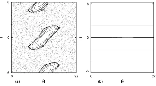
Figure 2.2: (a) GSM Poincar´e section forρˆ= 3.9 andK= 8.0 (pointP0 in figure 2.1): no spanning KAM
curves are observed. (b) GSM Poincar´e section forρˆ= 5.52andK= 8.0 (pointP1 in figure 2.1): spanning
KAM curves are restored.
The effect of chaos suppression is illustrated by Figs. 2.2(a)-(b). Figure 2.2(a) shows
a GSM Poincar´e section for the parameter values ˆρ= 3.9 and K = 8.0, which correspond
to the pointP0 in Fig. 2.1. No spanning KAM curves are observed in the Poincar´e section
as P0 belongs to the region of global chaos. Keeping the same value of K and changing
the ˆρvalue toρ2 (pointP1 in Fig. 2.1) elliminates all the chaotic orbits (see figure 2.2(b)).
2.3
Gyro-averaged standard nontwist map (GSNM)
As a second example of the gyro-averaged drift wave map, we introduce the gyro-averaged standard nontwist map (GSNM), which corresponds to a non-monotonic radial eletric field. The equilibrium potential is defined by:
φ0(x) = α
x
L
− 13Lx3
, (2.23)
whereα and Lare dimensional constants. The gyro-average of (2.23) results in:
hH0(x)iϕ =
α B0
x
L 1−
ρ2
2L2
− 13Lx3
and from (2.13):
Ω (x) = α
B0L
(" 1− ρ √ 2L 2#
−Lx2
)
(2.25)
The frequency Ω (x) has a non-monotonic parabolic profile with a maximum critical point
atx= 0. Forρ = 0, the zeros of Ω (x) (and also of the Er profile) are located at −L and
+L, whereL is thecharacteristic length of the frequency profile. Substituting (2.25) into (2.12), we obtain:
xn+1 =xn+
2π ω0B0
AkJ0(kρ) sin (kyn) (2.26)
yn+1 =yn+
2π ω0B0
α L (" 1− ρ √ 2L 2#
−xnL+12
)
. (2.27)
Introducing the dimensionless variables:
I =−x
L, θ=
ky
2π, (2.28)
we get the gyro-averaged standard nontwist map (GSNM):
In+1 =In−bJ0(ˆρ) sin (2πθn) (2.29)
θn+1 =θn+a
1−ρ¯
2
2
−In2+1
, mod 1 (2.30)
where:
a= αk
ω0B0L, b=
2πaA
α , (2.31)
¯
ρ= Lρ, ρˆ=kρ, (2.32) are four dimensionless parameters. We refer to b as the perturbation parameter, which is proportional to the amplitude A of the drift waves. Like in the GSM case, we can also
define an effective perturbation parameter:
bef =bJ0(ˆρ). (2.33)
The parameters ˆρand ¯ρ, as indicated by equations (2.32), correspond to the Larmor radius
ρ normalized using two different length scales: ˆρ is proportional to the ratio between ρ
2.3.1
Fixed Points
We now study FLR effects on the position and stability of the fixed points of the
GSNM, I∗ = I
n+1 = In and θ∗ = θn+1+m = θn, which, according to equations
(2.29)-(2.30), satisfy:
0 =bJ0(ˆρ) sin(2πθ∗), (2.34)
m =a
1− ρ¯
2
2
−I∗2
, (2.35)
wherem is an integer number. For each m∈Z, a= 0,6 bJ0(ˆρ)6= 0, and ¯ρ≤
q
2 1− m a
,
there are four fixed points:
P±= (0,±I∗(¯ρ)), (2.36)
Q± =
1
2,±I∗(¯ρ)
, (2.37)
where:
I∗(¯ρ) = √1
2
r
21− m
a
−ρ¯2. (2.38)
The θ coordinate of P± and Q± does not depend on any parameters. For fixed m and a, the I-coordinate depends only on ¯ρ and can be determined by using the function (2.38).
If ¯ρ =q2 1− ma, the pair of points {P+, P−} collide at (0,0), and {Q+, Q−} collide at
1 2,0
. Figure 2.3 shows theI-axis position of both pairs form= 0 and increasing ¯ρ. The
collision occurs for ¯ρ=√2. For higher values of ¯ρ, the fixed points don’t exist. The stability of a k-periodic orbit of a mapM is determined by the residue:
R= 1 4
"
2−T r
k−1
Y
i=0
J(~xi)
!#
(2.39)
whereJ is the Jacobian matrix ofM, evaluated at all points of thek-period orbit{~xi}ki=0−1.
If 0 < R < 1, the periodic orbit is elliptic (stable); if R < 0 or R > 1, it is hyperbolic
(unstable); and, finally, it is parabolic in the transition from one case to the other, which occurs for R= 0 or R= 1.
Applying formula (2.39) to the GNSM fixed points (2.36)-(2.37), we have:
Figure 2.3: CoordinateI of fixed points for m=0 and increasingρ¯. The fixed points collide forρ¯=√2 and cease to exist for higher values ofρ¯.
The stability of the fixed points{P±, Q±}withm = 0 can be analyzed using the parameter Λ (a, b,ρ,ˆ ρ¯) = R(P−). As shown in Fig. 2.4, depending on the value of Λ, there are three possible configurations. The symbol “x” denotes an hyperbolic point, and “o” an elliptic
point. The points have their stability inverted when −1 < Λ < 0 (configuration II), as indicated in figure 2.4b. All the fixed points are hyperbolic in configurationIII (fig. 2.4c), which occurs for Λ<−1 or Λ>1.
2.3.2
Separatrix reconnection
The location and stability of the fixed points determine the different phase space
topologies of the GSNM. These topologies, illustrated in Figs. (2.5a)-(2.5c), are
charac-teristic of nontwist maps and are called heteroclinic, separatrix reconnection, and homo-clinic [19]. Since the Larmor radius changes the stability of the fixed points, it is expected that it will also change the topology. Figures 2.5(a)-(c) show the heteroclinic-type,
separa-trix reconnection, and the homoclinic-type topologies in Poincar´e sections of the GSNM.
We adopt different values of a and b, and keep ˆρ and ¯ρ fixed.
To determine the condition for separatrix reconnection associated to the fixed points
(a) Configuration I: 0<Λ<1 (b) Configuration II:−1<Λ<0
(c) Configuration III: Λ<−1 or Λ>1.
Figure 2.4: Stability of the fixed points pointsP± andQ±withm= 0.
the fixed points by the Hamiltonian:
H(I, θ) = a
I
1− ρ¯
2
2
− I
3
3
− b
2πJ0(ˆρ) cos (2πθ), (2.41)
For 0 <Λ<1 (configuration I), separatrix reconnection occurs when H(P+) =H(Q−).
If −1 < Λ < 0 (configuration II), reconnection is observed when H(P−) = H(Q+).
Combining these two conditions, we obtain thereconnection line:
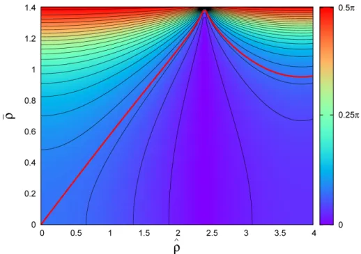
a= 3
4πσ(ˆρ,ρ¯)b, (2.42)
with slope:
σ(ˆρ,ρ¯) = |J0(ˆρ)| 1− ρ¯22
3 2
. (2.43)
The reconnection line divides the a −b parameter space in two regions: one with heteroclinic-type topology (a
b >
3
4πσ(ˆρ,ρ¯)) and another with homoclinic-type topology
(a) Heteroclinic-type topology with a = 0.0796 andb= 0.125.
(b)Separatrix reconnection witha= 0.0478 andb= 0.2.
(c) Homoclinic-type topology with a = 0.0239 andb= 0.3.
Figure 2.5: GSNM phase space topologies associated with the fixed points P± andQ± withm= 0. In all
arctan 3
4πσ(ˆρ,ρ¯)
. Keeping a and b fixed, the topology of the phase space remains
un-changed if the parameters ˆρand ¯ρ vary over an isoline. As an example, consider the case
for fixedaand bsuch thata= 3
4πb, which correponds to the reconnection condition in the
standard nontwist map [19]. In this case, there is always a reconnection for any values of
ˆ
ρ and ¯ρ over the red isoline of Fig. 2.6. The red isoline crosses the point ˆρ = ¯ρ = 0, at
which the GNSM reduces to the standard nontwist map. For high (red) values of σ, the
slope of the reconnection line approaches π
2, and the phase space is characterized by the
homoclinic-type topology for a fixed a and almost every value of the parameter b. For
low (blue) values of σ, the slope of the reconnection line tends to 0, and the phase space
is characterized by the heteroclinic-type topology for a fixedb and almost every value of
the parameter a.
Figure 2.6: Isolines of arctan3
4πσ(ˆρ,ρ¯)
: varying ρˆandρ¯along isolines does not change the topology of
the phase space. For high (red) values ofσ, homoclinic-type topology is observed for a fixed a and almost
every value of b. For low (blue) values of σ, heteroclinic-type topology is observed for a fixed b and almost
2.3.3
Nontwist transport barrier
The transition to global chaos in the GSNM occurs with the destruction of the non-twist transport barrier (NTB). One of main properties ofnontwist 3/2-degrees of freedom Hamiltonian systems, the NTB is a robust non-chaotic region of spanning KAM curves
dividing the phase space. The NTB isrobust in the sense that their spanning KAM curves are more resistant to perturbation than the other spanning KAM curves in the system.
NTBs are observed in both continuous in time Hamiltonian systems, and time discrete
area preserving models. The GSNM is an example of such a discrete model.
Let us consider the following form of Hamiltonian systems with 3/2 degrees of freedom
corresponding to a time-dependent perturbation of a one degree of freedom Hamiltonian:
H =H0(I) +ǫV (I, θ, t) (2.44)
where I and θ are the action-angle variables of the integrable system, H0, and the
pa-rameter ǫcontrols the strength of the time-periodic pertubative termV. In this case, the
twist or non-degenerate condition is given by:
dΩ
dI = d2H
0
dI2 6= 0, (2.45)
for all I. If there is at least one critical or degenerate point in the frequency profile, i.e. points such that dΩ/dI = 0 for I = Ic, the non-degenerate condition is violated, and
the system defined by (2.44) is called as a nontwist ordegenerate 3/2-degrees of freedom Hamiltonian system.
One of the main properties of such systems is the presence of NTBs, one for each
degenerate point of the frequency profile. This property was described originally in Ref.
[19] and was called banded chaos. A more recent work referred to the same property as strong Kolmogorov-Arnold-Moser stability [23]. In this case, the phase space can be almost completely occupied by chaotic orbits, but robust spanning KAM curves forming
constitute the NTB can still be present.
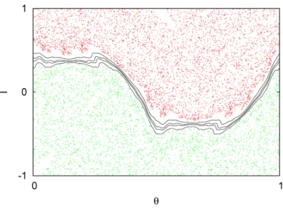
Figure 2.7 shows a GSNM Poincar´e section with a NTB. The Poincar´e section
pre-sented in figure 2.7 is the same for any values of b and ˆρ such that: a = 0.354, ¯ρ = 0,
Figure 2.7: Nontwist transport barrier in the GSNM: robust region of spanning KAM curves (black curves) splitting the phase space in two chaotic regions, indicated by the red and green orbits.
orbits (green and red regions), but it has a robust “belt” of spanning KAM curves (black
curves). As we have already seen, the GSNM can be obtained by integrating the equations
of motion of the 3/2-degrees of freedom Hamiltonian (2.8) with a frequency defined by
(2.25). The Hamiltonian system is degenerate because its frequency has a critical point
(a maximum located atx= 0).
2.3.4
Breakup Diagrams
Here we study the transition to global chaos in the GSNM, which is related to the
destruction of the robust spanning KAM curves that constitute the NTB. It is important
to remark that the transition to global chaos in nontwist systems is still an open problem.
However, a possible approach to this problem consists of estimating the parameter values,
or the critical thresholds, that determine the breakup of theshearless KAM curve. We say that a KAM curve isdestroyed orbroken when it becomes chaotic by changing parameter values.
The shearless curve, in absence of perturbation, is the KAM curve located at the value
of action variable that violates the twist condition and defines a degenerate point in the
developed in [23], the shearless curve corresponds to a “degenerate tori”, which has the
same robustness properties that characterizes the NTB’s spanning KAM curves. Thus, we
can say that the shearless curve belongs to the NTB, and the parameters values related
to the NTB destruction can be estimated from the parameter values that determine the breakup of shearless curve.
A standard way to determine the parameter values of shearless curve’s breakup is based
on the indicator point (IP) method (see, for example, Refs. [6, 21, 38, 40]). This method consists on finding the parameter values for which the iterations of the indicator point,
which defines the indicator point orbit (IPO), are chaotic. If the IPO is quasiperiodic, it covers a shearless KAM curve. When the IPO is chaotic, the shearless curve is broken.
The indicator points can be found in nontwist maps with special symmetries by computing
the fixed points of transformations of the reversing symmetry group. Further details can be found in Ref. [39].
Using the same arguments and a procedure similar to the one in [40], which shows
how to obtain the IPs for the standard nontwist map (see Appendix B of Ref. [40] and
also Appendix B at the end of this work for more details), we obtain the following IPs for
the gyro-averaged standard nontwist map:
z01 =
1 4,+
bJ0(ˆρ)
2
, z02 =
3 4,−
bJ0(ˆρ)
2
, (2.46)
z11 =
a
2
1− ρ¯
2
2
+1
4 mod 1, 0
, z12 =
a
2
1−ρ¯
2
2
+ 3
4 mod 1,0
.
(2.47)
Once the IPs are found, the next step is to obtain the critical thresholds using an
appro-priate criterion to determine if the IPO is chaotic. Our criterion is based on the technique
proposed in [28], which considers therecurrence properties of the IPO in conjunction with Slater’s Theorem [29]. Recurrence properties and their relation to the Slater’s Theorem
were also discussed in [30]. In Ref. [31], the technique described in [28] was used to study
the breakup of the shearless curve in the nontwist standard map.
The Slater’s Theorem states that, for any quasiperiodic motion on the circle, there are
two-dimensional systems, once the dynamics on a KAM curve is mapped to a quasiperiodic
rotation on a circle [28]. The recurrence time is defined as the number of iterations that an orbit takes to return to a neighbourhood of a point. Our procedure to characterize the
dynamics of an indicator point orbit of the GSNM is the following: with any one of the
indicator points as the initial condition, we compute the orbit for a numberN of iterations
and choose the point of the orbit which has the maximum number of different recurrence
times. If there are more than three different recurrence times, we conclude that the orbit
is chaotic and the corresponding KAM curve is destroyed.
More precisely, the procedure consists of the following steps:
• Compute the orbit O = {uk}Nk=0 with initial condition u0 = z11, where N is the
number of iterations.
• Construct the recurrence matrix 2:
Rij = Θ(ǫ− kui−ujk), (2.48)
wherei, j ∈ {0, ..., N},ui, uj ∈O, Θ is the Heaviside function, andǫ is a parameter
defining the size of the neighbourhood. If the distance beetweenui and uj, given by
the norm kui−ujk, is less than ǫ,Rij = 1; otherwise, Rij = 0.
• Define the recurrence timeτij asτij =|i−j| such thati 6=j and Rij = 1. That is,
there is a recurrence timeτij if the orbitO crosses the neighbouhood ofuj at thei-th
iteration. For each point uj, compute the set of recurrences SR(j) = ∪Ni=0,i6=j{τij}.
Note that just different recurrence times belong to SR(j)
• Determine the maximum number of different recurrence times:
nR =max
n
nSR(j)oN
j=0, (2.49)
where n is the number of recurrence times belonging to SR(j), and use the Slater’s Theorem to conclude that the orbitO is chaotic if nR>3.
2Here we borrow the definition presented in Ref. [30] of the binary matrix R. Its graphical
rep-resentation, called recurrence plot, can be used to analyse the recurrence properties of any dynamical
FornR≤3, the characterization of the dynamics using the Slater’s Theorem is
incon-clusive because the orbit might be periodic, quasiperiodic or even chaotic. In this case,
we can increase the number of iterations, N, to explore if nR increases beyond 3. If the
condition nR ≤3 still persists and no change innR is observed, we assume that the orbit
is periodic for nR = 1 and quasiperiodic for nR = 3. The condition nR = 2 requires a
more careful analysis with higher values N. Increasing N, nR stabilizes in 3, indicating
quasiperiodic dynamics, or assumes values greater than 3, which is the case for chaotic
dynamics. Although more rigourous criteria for the casenR≤3 are lacking, the numerical
results of Refs. [28, 30] support the use of the recurrence properties and their relation to
the Slater’s Theorem as a computationally fast diagnostic to recognize chaotic motion.
We now apply this diagnostic to compute breakup diagrams for the GSNM show-ing regions in the parameter space where the shearless curve is broken. The diagrams
were constructed by applying the procedure described above to IPOs generated with
dif-ferent values of the GSNM parameters. Each set of values corresponds to a point on
2-dimensional parameter space. Since the GSNM has four parameters, the breakup
dia-grams are constructed varying two parameters at a time while keeping the others constant.
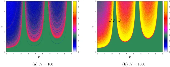
Our first examples are presented in Figs. 2.8a and 2.8b. In both diagrams, we used a grid
of 1000×1000 points and vary b and ˆρ. We fix ¯ρ = 0 (which means that ρ ≪ L ) and
a = 0.1. For each point on the grid, the IPO and its nR are computed for ǫ = 0.1. The
color of each point is defined by the value of nR. The relation between the colors and
the nR values is indicated in the color palette. For example, blue corresponds to nR= 1;
dark-blue, nR = 2; green, nR = 3; magenta, nR = 4; and all points with nR ≥ 9 are
plotted in yellow.
To construct diagram 2.8a, we used N = 100. Although the number of iterations is
increased to N = 1000 in diagram 2.8b, the main geometric features that enable us to
distinguish between regular and chaotic dynamics are mantained. The main difference is
observed in points with nR = 2 (dark-blue points). Increasing the number of iterations,
most of these points have their color changed corresponding to nR > 3. Diagram 2.8a
shows that, even for a low number of iterations, it’s possible to identify the breakup of
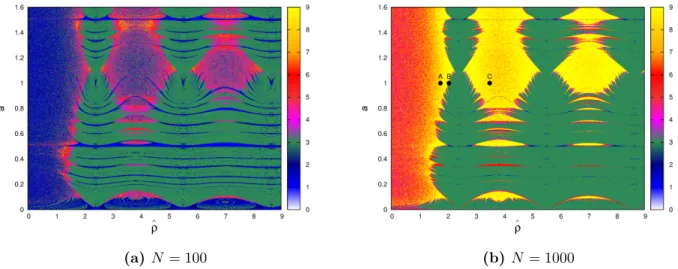
(a)N = 100 (b) N= 1000
Figure 2.8: GSNM breakup diagrams for ρˆ versus b, with ρ¯ = 0, and a = 0.1. For each point (ˆρ, b) in the diagram, the IPO and the correspondentnR are computed with ǫ= 0.1. The color pallete indicates the
value ofnR. The breakup of the shearless curve can be detected in the points where nR >3. The IPO is
quasiperiodic in the green region (nR= 3) which corresponds to low effective perturbation bef, i.e, lowb or
ˆ
ρnear a zero ofJ0.
magenta, red, and yellow colors. Green points (nR = 3) are concentrated in domains
with low effective perturbationbef, which means a low perturbationb or ˆρ close to a zero
of the zero-order Bessel function. As verified in Figs. 2.9(a)-(c), nR = 3 (green points)
corresponds to quasiperiodic IPOs. For points outside the green region (e.g. point A in
Fig. 2.8b), the IPO is chaotic, and, as shown in Fig. 2.9a, the shearless curve is destroyed.
Changing ˆρ to a value near a zero ofJ0 such that the point moves inside the green region
(e.g. pointB of Fig. 2.8b), the shearless KAM curve is restored because the IPO becomes
quasi-periodic, as shown by the red orbit in Fig. 2.9b. Figure 2.9c shows that the shearless
KAM curve is broken again for parameter values outside the green region (e.g. point C
in Fig. 2.8b).
Breakup diagrams with varying a and ˆρ are shown in figures 2.10a and 2.10b. The
number of iterations adopted to construct the first diagram was N = 100. In the second
diagram, we increased the number of iterations toN = 1000. As before, the green points
(nR = 3), which are indicators of non-chaotic dynamics, are concentrated near the zeros
of J0. A high occurrence of points with nR = 3 is also observed in regions with low a.
(a)ρˆ= 1.75 (b)ρˆ= 2.2
(c) ρˆ= 3
Figure 2.9: The shearless KAM curve, identified through a quasiperiodic IPO (red orbit), is restored near the zeros of J0. Fixed parameters: a = 0.1; b= 3; ρ¯= 0. (a) For ρˆ= 1.75 (point A, figure 2.8b), the IPO is
chaotic. (b) Forρˆ= 2.2(point B), the IPO (red orbit) is quasiperiodic. (c) Forρˆ= 3(point C), the shearless
(a)N = 100 (b) N= 1000
Figure 2.10: GSNM breakup diagrams for ρˆversusa, withρ¯= 0 andb= 1.5. Neighbouhood size: ǫ= 0.1. Green points, corresponding to quasiperiodic dynamics, are concentrated near the zeros ofJ0and in domains
with lowa.
the main geometric features remain the same, although many of the blue points (nR = 1
ornR= 2) have their colors changed such that nR >3. Poincar´e sections for parameters
corresponding to points A, B, and C in Fig. 2.10b are shown in figures 2.11a-c. As
expected, the shearless KAM curve is broken at points A and C, and restored at point
B.
Additional examples of breakup diagrams are presented in figures 2.12a-d. The
param-eters are the same as those in Figs. 2.8b and 2.10b, but the value of the fixed parameter ¯ρ
is higher. Comparing figures 2.12a-b to 2.8b, we see that increasing ¯ρincreases the number
of green points (nR = 3) and the robustness of the shearless KAM curve. That is, higher
values of the perturbation parameter b are required to make the IPO chaotic. As shown
in Figs. 2.12c-d, the distribution of points with nR = 3 is changed with the increasing
of ¯ρ, resulting in different critical thresholds but with no significant suppression of green
points. Red and yellow points disappear in certain regions and reappear in others, as can
be seen by comparing Figs. 2.10b, 2.12c and 2.12d.
Summarizing: in this section we used a computational technique based on the
recur-rence properties of the IPO to estimate the critical parameter values for the breakup of
(a) ρˆ= 1 (point A) (b)ρˆ= 2.05 (point B)
(c) ρˆ= 3.5 (point C)
Figure 2.11: Poincar´e sections of the GSNM map for points A, B and C, in the diagram 2.8b. The shearless KAM curve corresnponding to point B is present, but it breaks at A and C. Fixed parameters: a= 1;b= 1.5;
¯
(a) ρ¯= 0.8;a= 0.1 (b) ρ¯= 1.2;a= 0.1
(c)ρ¯= 0.8;b= 1.5 (d)ρ¯= 1.2;b= 1.5
Figure 2.12: Diagram: (a) and (b): the robustness of the shearless KAM increases whenρ¯increases, which means that more green points (nR = 3) are observed. Diagrams (c) and (d): the critical thresholds change
the role of the Larmor radius in the destruction and formation of shearless spanning KAM
curves. FLR effects were studied by varying the parameters ˆρ or ¯ρ. When ˆρ is close to a
zero ofJ0, the shearless curve becomes more robust to perturbation in b. An explanation
for this effect is that, no matter how high the values of b are, the zeros of J0 make the
GSNM’s Hamiltonian integrable, as seen in equation (2.8). As ˆρ approaches a zero of
J0, the shearless curve and the other spanning KAM curves that make up the nontwist
transport barrier are restored. Another FLR effect is observed by changing the parameter
¯
ρ. As can be seen in Figs. 2.12a-b, the robustness of the shearless curve and the critical
thresholds can also be modified by increasing ¯ρ.
2.4
Gyro-averaged quartic nontwist map (GQNM)
In this section, we propose another area-preserving map, the gyro-averaged quartic
nontwist map (GQNM). A key property of the GQNM is that it has a zonal flow bifur-cation, similar to the one observed in the nontwist Hamiltonian system of Ref. [6]. The Hamiltonian system in [6] is a drift-wave model of the E× B transport with FLR ef-fects, and the zonal flow bifurcation corresponds to a bifurcation of the maximum of the
frequecy’s profile that occurs when the Larmor radius increases.
As in the previous maps, the GQNM equations are obtained from the gyro-averaged
drift wave map in equations (2.11) and (2.12). Here we adopt an equilibrium potential
similar to the one proposed by [6]:
φ0(x) = αtanh
x
L
, (2.50)
where α and L are dimensional constants. Applying the gyro-average operation (2.4) to
(2.50), we have:
hH0(x)iϕ =
α
2πB0
Z 2π
0
tanhx
L + ρ Lcosϕ
dϕ. (2.51)
The nonlinear frequency, according to (2.13), is defined by:
Ω (I) = α 2πLB0
Z 2π
0
sech2(I+ ¯ρcosϕ) dϕ, (2.52)
where I = x/L, and ¯ρ =ρ/L. The zonal flow bifurcation occurs due to a bifurcation of
Figure 2.13: Bifurcation of the critical point in the frequency profile (2.53)
methods or approximated by Taylor expansions. To analyse, in a simple way, the FLR
effect on the zonal flow in (2.52), we consider the following approximation:
Ω (I) = α
LB0
1−I2
1−ρ¯2
3
2 1−I
2
−1
, (2.53)
valid for small values of |I|and ¯ρ. Figure 2.13 shows profiles of (2.53) for different values of ¯ρ. For ¯ρ = 0, there is only one critical (Ω′ = 0) maximum point, located at I = 0.
Increasing ¯ρ leads to the increasing the profile’s “flatness”, followed by a critical point
bifurcation, where the maximum becomes a minimum and two maxima appear. The
bifurcation threshold ¯ρb can be determined from the condition:
∂2Ω
∂I2
I=0,ρ¯=¯ρb
= 0. (2.54)
The second-order derivative of (2.53) is given by:
∂2Ω
∂I2
I=0
=−2 + 4¯ρ2. (2.55)
From (2.54) and (2.55), it follows that the bifurcation threshold occurs at:
¯
ρb = 1/ √
2. (2.56)
the GQNM:
In+1 =In+bJ0(ˆρ) sin (2πθn), (2.57)
θn+1 =θn+a 1−In2+1
1−ρ¯2
3
2 1−I
2
n+1
−1
, mod 1, (2.58)
where a=kα/ω0LB0, andb, the perturbation parameter, is given byb = 2πaA/α. As in
the previous maps, an effective perturbation parameter can be defined as bef = bJ0(ˆρ).
Like the GSNM, the GQNM reduces to the standard nontwist map for ˆρ = ¯ρ = 0. In
what follows, we discuss FLR effects on the GQNM’s fixed points and nontwist transport
barriers.
2.4.1
Fixed Points and nontwist transport barriers
In a similar way as we have done for the GSNM (section 2.3.1), FLR effects on the
location and stability of period-1 orbits can be analysed in the GQNM. The fixed points
(θ∗, I∗) of the GQNM satisfy:
0 =bJ0(ˆρ) sin (2πθ∗) (2.59)
m=a 1−I∗2
1−ρ¯2
3
2 1−I
∗2
−1
, m∈Z (2.60)
Form = 0, which corresponds to the simplest case,a6= 0, and bJ0(ˆρ)6= 0, there are four
fixed points, given by:
P1±= (0,±1), Q±1 =
1 2,±1
(2.61)
If ¯ρ≥2¯ρb = √
2, there is an adittional set of fixed points:
P2±= (0,±h(¯ρ)) Q±2 =
1
2,±h(¯ρ)
(2.62)
where the function h(¯ρ) is defined by:
h(¯ρ) =
s
(¯ρ2 −2)
3¯ρ2 (2.63)
Figure 2.14 shows the I coordinates of the fixed points with m= 0. P1± and Q±1 exist for all ¯ρ ≥ 0 and are always located at I = ±1. P2± and Q±2 only exist for ¯ρ ≥ 2¯ρb =
√
Figure 2.14: I coordinates of fixed points with m= 0. The set P1±, Q
±
1 is fixed in theI-axis and exists
for anyρ¯≥0. The setP2±, Q
±
2 only exists forρ¯≥2¯ρb=
√
2
and their positions in the I axis are determined by the function h(¯ρ), which satisfies
0≤ h(¯ρ) < √1
3. The stability of the fixed points
P1±, Q±1, P2±, Q±2 can be analysed by evaluating the Greene’s residue (2.39):
R P1±=−R Q±1=∓Λ (a, b,ρ,ˆ ρ¯) (2.64)
R P2±=−R Q±2=±h(¯ρ) Λ (a, b,ρ,ˆ ρ¯) (2.65)
where the function Λ (a, b,ρ,ˆ ρ¯), which corresponds to the residue of P1−, is given by:
Λ =πabJ0(ˆρ) 1 + ¯ρ2
(2.66)
Given the values of the parameters a, b, ˆρ, and ¯ρ, we can determine the residue of P1−, and then, using equations (2.64)-(2.65), compute the residues of the other fixed points
P1+, Q±1, P2±, Q±2 . As shown in Fig. 2.15, depending on the value of Λ, there are five possible stability configurations. The number of elliptic fixed points reduces when Λ
increases, and the first points to lose stability are the outer ones. In the configuration
V (figure 2.15e), which occurs for |Λ|> h(¯1ρ), all the fixed points are hyperbolic. A final remark is regarding the strong stability of the elliptic points in configurations III and IV
associated to the elliptic points can still survive once the limit 1
h(¯ρ) goes to infinity when
¯
ρ→√2+ (¯ρ greater than and close to √2).
An important consequence of the zonal flow bifurcation is the occurrence of nontwist barrier bifurcations. In particular, instead of just one NTB, two additional NTBs appear after the zonal flow bifurcation, which occurs when ¯ρ increases. The NTB bifurcation is
illustrated in Figs. 2.16a and 2.16b: for ¯ρ . ρ¯b, only one region with robust spanning
KAM curves is present (Fig. 2.16a); increasing ¯ρ such that ¯ρ > ρ¯b (Fig. 2.16b), two
additional NTBs appear. The outer NTBs are separated from the central one by two
regions of confined chaotic orbits.
2.4.2
Robustness of the central shearless curve
Our interest in studying the robustness of spanning KAM curves as function of b
resides on the fact that this parameter is proportional to the amplitude of the drift waves.
For a very small Larmor radius (or in the absence of FLR corrections), high amplitude
values can easily destroy all spanning KAM curves, what is not always the case when
FLR effects are taken into account. As mentioned in section 2.3.3, the robustness of the
GSNM’s shearless curve can be significantly increased if ˆρ is near a zero of J0. In this
case, the effective perturbation bef is small, what explains the robustness of the shearless
curve even for high values of b. The same effect is present in the GQNM, as we can see
in equation (2.57).
Figures 2.17(a)-(d) show breakup diagrams for the central shearless KAM curve as
function of b and ¯ρ. In all cases, bef is small, because the values of ˆρ are close to the
zeros ofJ0. Under this condition, and when ¯ρ is near the zonal flow bifurcation threshold
¯
ρb, defined in (2.56), a significant increasing of the robustness of the shearless curve is
observed. For ¯ρ < ρ¯b, higher values of b are required to the breakup as ¯ρ approaches ¯ρb.
However, for ¯ρ >ρ¯b, the robustness diminishes as ¯ρincreases. Therefore, the central NTB
robustness can be increased not only by approximating ˆρto any of the J0’s zeros, but also
by making ¯ρ close to ¯ρb.
It is interesting to note that, in the neighbourhood of I = 0, the degree of “flatness” of
(a)I: 0<Λ<1 (b) II: −1<Λ<0
(c) III: 1<Λ< 1
h( ¯ρ) (d) IV:− 1
h( ¯ρ)<Λ<−1
(e) V: Λ<− 1
h( ¯ρ) or + 1
h( ¯ρ)<Λ
Figure 2.15: Depending on the value ofΛ, there are five possible configurations characterizing the stabillity of the period-one fixed pointsP1±, Q
±
1, P
±
2 , Q
±
(a) ρ¯= 0.707 (b) ρ¯= 1.42
Figure 2.16: (a) One NTB forρ¯.ρ¯b. (b) After the zonal flow bifurcation, three NTBs can be observed.
Parameters: a= 0.5;b= 1.35;ρˆ= 2.8.
curve, the degree of “flatness” is higher near the bifurcation threshold, but it becomes
smaller otherwise. The flatness around I = 0 can be measured through |Ω′′(0)|, which
corresponds to the absolute value of the second-order derivative of Ω aroundI = 0. A high
degree of flatness around I = 0 means a small value of |Ω′′(0)|. Based on these results,
we conjecture that the robustness of NTBs in nontwist symplectic maps depends on the
flatness of the frequency profile around the points of maximum or minimum (critical
points), and that, for small perturbation, the robustness increases with the degree of
flatness.
In section 2.3.3, we mentioned that the robustness of a NTB is related to the
phe-nomena referred to as strong KAM stabillity [23]. The strong KAM stabillity argument is based on the idea of overlapping of resonances, as presented by [32], to explain the
destruction of invariant tori (spanning KAM curves). Tori located between neighbouring
resonances break up when the resonances overlap. Thus, one expects that tori are more
resilient to perturbation whenresonance widths are smaller. As shown in [23], in 3/2 de-grees of freedom nontwist Hamiltonian systems, the width,δΩ, of second-order degenerate
resonances scales as:
δΩ∼[ǫ|Ω′′(I0)|]2/3, (2.67)
(a)a= 0.5; ˆρ= 5.47;ρ2= 5.52 (b) a= 3; ˆρ= 8.67;ρ3= 8.65
(c)a= 10; ˆρ= 11.80;ρ4= 11.79 (d)a= 30; ˆρ= 2.42; ρ1= 2.40
Figure 2.17: For smallbef values, the robustness of the central shearless curve (and, thus, also of the central
NTB) increases with the degree of flatness of the frequency’s profile around the critical point. The flatness can
be controlled by the parameterρ¯and becomes higher whenρ¯is close to the zonal flow bifurcation threshold
¯
ρb (shown with the solid black vertical line). The values ofbef are made small by settingρˆclose to the zeros
which:
Ω′(I0) = 0, Ω′′(I0)6= 0. (2.68)
As we have seen in section 2.3.3 (see eq. (2.45)),I0in (2.68) corresponds to the value of the
action variable for which the frequency’s profile violates the twist condition. Forǫ= 0, the
shearless KAM curve is located exactly atI0. If the system is slightly perturbed,
second-order degenerate resonances appear along the neighbourhood of the shearless curve. When
these resonances overlap, the shearless curve breaks up.
The central shearless curve of the GQNM is associated to the critical point located
at I0 = 0. At this point, the frequency’s profile, defined by (2.53), satisfies (2.68) for
any ¯ρ 6= ¯ρb. Thus, in the Hamiltonian system from which the GQNM equations are
derived, second-order degenerate resonances might appear near the central shearless curve.
According to (2.67) and (2.55), the width of second-order resonances has the property:
lim
¯
ρ→ρb¯ δΩ = 0, (2.69)
because, for ¯ρ close to ¯ρb, |Ω′′(I0)| vanishes. Small values of |Ω′′(I0)| result in small
degenerate resonance widths and a more robust central shearless curve. As |Ω′′(I
0)| is
directly related to the flatness of the frequency’s profile aroundI0 (a small|Ω′′(I0)|means
more “flatness” aroundI0), formula (2.67) is consistent with the results showed in figures
2.17(a)-(b) and supports our conjecture relating high robustness of the shearless curve to
non-monotonic frequency profiles with high flatness around degenerate points.
It is important to remark that the same arguments developed in this section can be
applied to interpret the results presented in Ref. [36], in which the authors study the effect
of shearless safety factor profiles on the confinement properties of magnetic field lines in
Tokamaks. In the 1 + 1/2 degrees of fredom Hamiltonian model adopted to describe
magnetic field lines, the safety factor q is characterized by regions with vanishing shear
that makes the system of a nontwist kind because the q-profile is inversely proportional
to the nonlinear frequency of system. In Ref. [36], the authors analyze the influence of
the amount of flatness in low shear regions of theq-profile on the robustness of the NTBs.
Changing the form of theq-profile, the flatness can be increased, and a more robust NTB
Statistical Properties of the GSM
Model
In this chapter we study statistical properties of a GSM based model where the effective
perturbation is considered a random variable. Section 3.1 describes the basic assumptions
and equations of the model. In section 3.2, the first set of results related to statistics of
the effective perturbation are presented: we obtain the gamma’s pdf, analyze its main
properties and also histograms of gamma for different values of the thermal Lamor radius.
The moments, as well the average and dispersion of gamma, are presented in section
3.3. Section 3.4 describes the analytical and numerical results related to the cumulative
distributive function of gamma, which is used in section 3.5 to obtain the probability
of global chaos. We study the escape rate in section 3.6, and the rate of trapping by
period-one islands in section 3.7. This chapter is partly based on Ref. [42].
3.1
GSM Model
In the GSM model, particles are assumed to follow orbits described by gyro-averaged
standard maps with effective perturbation values which are not necessarily the same.
These values differ randomly from one to other particle and are constant in time. The
model comes from the idea of considering an ensemble of particles whose Larmor radii are
randomly defined and kept constant in time.
Therefore, the dynamics of each charged particle in the GSM model is determined by:
In+1 =In+K(ˆρ) sinθn, θn+1 =θn+In+1, mod 2π, (3.1)
whereK, the effective perturbation, is a random variable defined by:
K =K0J0(ˆρ), (3.2)
and K0 denotes the perturbation parameter, which is a constant and the same for all
particles of the ensemble 1.
In a similar a way as done in [6, 9], we assume plasmas in thermal equilibrium and
a Larmor radius’ pdf resulting from the Maxwell-Boltzmann distribution. The Larmor
radius’ pdf characterizes the statistics of the random variable ˆρ and can be obtained as
follows.
3.1.1
Maxwell-Boltzmann Distribution
The Maxwell-Boltzmann distribution is given by [43]:
F(~v) = n
β
2π
3 2
exp
−β2~v2
, (3.3)
where~v is the three-dimensional particles’ velocity and n is the number of particles per
unit volume. The parameter β is defined by:
β = kBT
m , (3.4)
wherekB is the Boltzmann constant,T is the absolute temperature andmdefines the
par-ticle’s mass. Equation (3.3) represents the most probable distribution function satisfying
the macroscopic conditions or constraints imposed on the system [43].
According to (3.3), the probability density function of the particle’s velocity in one
dimension is a Gaussian with zero mean (see [43] for details):
fi(vi) =
r
β
2πexp
−β2vi2
, (3.5)
1Although the set of Eqs. (3.1) corresponds exactly to th GSM, here we decided to change notation
used in the previous chapter to refer to the effective perturbation and the perturbation parameter. Kef
where the indexidenotes thex,y, andzcomponents of the velocity. The thermal velocity
is defined as [44]:
vth =
1
√
β. (3.6)
The thermal velocityvthcorresponds to the standard deviation of the particle’s velocity
in one dimension:
vth =σvi =
q
hv2
ii − hvii2. (3.7)
Equation (3.7) can be verified considering that hvii = 0 and computing the moment hv2
ii:
v2i =
+∞
Z
−∞
fi(vi)vi2dvi =
1
β. (3.8)
Using (3.7), equation (3.5) can rewritten as:
fi(vi) =
1
p
2πv2
th exp − v 2 i
2v2
th
. (3.9)
3.1.2
Larmor Radius’ PDF
The Larmor radius is defined by [44]:
ρ= v⊥ Ω0
, (3.10)
where the cyclotron frequency Ω0 is:
Ω0 = |
q|B0
m , (3.11)
and v⊥ corresponds to the perpendicular component of the particle’s velocity to the toroidal magnetic field lines:
v⊥=qv2
x+vy2. (3.12)
The probability of the perpendicular velocity assuming a value between v⊥ and v⊥+
a circular regionR of radiiv⊥ and v⊥+dv⊥, i.e.:
f⊥(v⊥)dv⊥ =
Z
R
fx(vx)fy(vy)dvxdvy (3.13)
= β 2π Z R exp
−β2 vx2+vy2
dvxdvy (3.14)
= β 2π 2π Z 0 exp −β 2v 2 ⊥
v⊥dθdv⊥. (3.15)
Thus, the perpendicular velocity’s pdf is:
f⊥(v⊥) = βv⊥exp
−β 2v 2 ⊥ (3.16)
The probability of finding the Larmor radius between ρ andρ+dρ isfL(ρ)dρ, where
fL is the Larmor radius’ pdf. According to Eq. (3.10), if we assume that the cyclotron
frequency is a constant and the same for all charged particles, then:
fL(ρ)dρ=f⊥(v⊥)dv⊥ (3.17)
=βΩ20ρexp
−βΩ
2 0 2 ρ 2 dρ (3.18) and:
fL(ρ) = βΩ20ρexp
−βΩ
2 0 2 ρ 2 (3.19)
Defining the thermal Lamor radius as:
ρth =
vth
Ω0
= 1 Ω0√β
, (3.20)
and substituting (3.20) in (3.19), we have:
fL(ρ) =
ρ ρ2 th exp " −1 2 ρ ρth 2# (3.21)
In chapter 2, we defined the normalized Lamor radius as ˆρ =kρ. According to (3.21),
the normalized Lamor radius’ pdf is then given by:
f(ˆρ) = ρˆ ˆ
ρ2
th
exp
"
−12