Hierarchal Variable Switching Sets of Interacting
Multiple Model for Tracking Maneuvering Targets in
Sensor Network
Fathy Aamer, and Seham Ebrahim
Department of Information Technology, Faculty of Computer & Information Cairo University Cairo, Egypt
Department of Computer Engineering, Modern Academy of computer engineering Cairo, Egypt
Abstract
Tracking maneuvering targets introduce two major directions to improve the Multiple Model (MM) approach: Develop a better MM algorithm and design a better model set. The Interacting Multiple Model (IMM) estimator is a suboptimal hybrid filter that has been shown to be one of the most cost-effective hybrid state estimation schemes. The main feature of this algorithm is the ability to estimate the state of a dynamic system with several behavior modes which can “switch” from one to another. In particular, the use of too many models is performance-wise as bad as that of too few models. In this paper we show that the use of too many models is performance-wise as bad as that of too few models. To overcome this we divide the models into a small number of sets, tuning these sets during operation at the right operating set. We proposed Hierarchal Switching sets of IMM (HSIMM). The state space of the nonlinear variable is divided into sets each set has its own IMM. The connection between them is the switching algorithm which manages the activation and termination of sets. Also the re-initialization process overcomes the error accumulation due to the targets changes from one model to another. This switching can introduce a number of different models while no restriction on their number. The activation of sets depends on the threshold value of set likely hood. As the likely hood of the set is higher than threshold it is active otherwise it is minimized. The result is the weighted sum of the output of active sets. The computational time is minimum than introduced by IMM and VIMM. HSIMM introduces less error as the noise increase and there is no need for re adjustment to the Covariance as the noise increase so it is more robust against noise and introduces minimum computational time.
Keywords: Interacting Multiple Model (IMM), Probabilistic Data Association, Sensor Network.
1. Introduction
Multiple-model approach provides the state-of the-art solutions to many problems involving estimation, filtering,
control, and/or modeling. One of the most important problems in the application of the multiple-model approach is the design of the model set used in a multiple-model algorithm. There are two types of multiple-model-set design: online and offline. Offline design is for the total model set or the initial model set in a variable-structure approach, as well as for the fixed structure approach. In a fixed-structure algorithm, the model set used cannot vary and is determined a priori by model-set design. In a variable-structure algorithm, the model set in effect at any time is determined by an adaptation process, known as model-set
adaptation, which may be viewed as an online (real-time)
design process and will depend on the total model set determined a priori if such a set exists. In this paper we study the IMM with a large number of operating modes and introduce its performance for different modes changes. Then we replace this IMM with another structure of IMM. The structure includes sets of IMM. Each set includes part of these operating modes. At initialization all the sets are active but the right set which introduce lower innovation will be active while the others will be switched off When the system change to a different active set the diverging of the active set will cause system initialization and activation to all sets and start to tune to the right set. This algorithm overcome the problem of large number of modes in IMM, activate only the right set not all sets which introduce less computation complexity, and allow variation of time step to large values to reduce energy consumption in Sensor Network while tracking.
2. The Related Work
The IMM was introduced in [1] which summarized the state-of-the-art of the IMM and its variants. They discuss and compare the base-line IMM algorithm with variable-structure variants, multiple sensor variants, correlated noise variants, glint-noise influenced variants, and others to know more about IMM. But it is shown theoretically that the use of too many models is performance-wise as bad as that of too few models. In [7] they introduced difficulties of excess of measure while [8] introduced the difficulties of using IMM in Radar system. In [2] they introduced limitations of the fixed structure algorithm. Then presented theoretical results pertaining to the two ways of overcoming these limitations. select/construct a better set of models and/or use a variable set of models. The new approach was illustrated in non stationary noise identification problem. In our previous work [12] considering Extended Kalman filter and IMM in the same tracking problem to introduce the accuracy and time delay of the two tracking algorithm. In this paper structure of IMM sets are introduced to overcome limited number of sets and nonlinearity of target motion model. The structure includes number of IMM (set of modes) working separately. But the right set will be considered while the others will be switched off.
3. The Interacting Multiple Model
The system is described by the model:
)), 1 ( , ( * )) 1 ( , ( ) ( )) 1 ( , ( ) 1
(k F kmk xk Gkmk ukmk
x (1)
), ( ) ( ) ( )
(k H k xk wk
z (2)
Where xnx is the system state vector, znz is the measurement vector, unu and wnz are mutually uncorrelated, white zero mean Gaussian noises with coveriances Qu and Rw respectively. The parameter mk
presents the current system mode.Fis the system dynamic matrix, andHis the measuring matrix.
Because the accurate system model is unknown, the system is described by a number of models. The event that theith
modelmiis actual at timekis denoted as
Mi(k)={m(k)=mi}.
It is assumed that the system model sequence is a Markov chain with transition probabilities
r i k
P
k P k m k m P
r
ij r
ij r i j
..., 2 , 1 ,
1 ) ( where
) ( ) ( | ) 1 (
1 j
Designing model set is the major element affects the performance of the IMM. These models represent different mode of operation of the system. If the system operating mode is fare from these models it doesn’t converge. Or if we add models near to each other in parameters the estimated state may converge to the wrong model and also
models probabilities after converging to the wrong model cause system divergence.
We introduce two models one linear motion and one coordinated turn model for quick maneuver detection.
1) Constant Velocity Model: This model is the most
commonly used. The target is assumed to move with a constant velocity. For notational simplicity,
}
,
,
,
{
x
t
x
t
y
t
y
t
t
x
refers to the state (coordinates and the velocities) of a single target following this motion model andu
t
is the corresponding motion noise.t t
t u
T T T T
x T T
x
0 2 0
0 0 2
1 0 0 0
1 0 0
0 0 1 0
0 0 1
2 2
1 (3)
where ~ (0, ( 2, 2) y x t N diag
u σ σ .
2) Coordinated Turn Rate Model:This model assumes that
the target moves with a constant speed (norm of the velocity vector) and a constant known turn rate
ω
. Again, we denotex
t
as the state of a single target from this classand
u
t
as the corresponding motion noise. To introduce the case of a target moving with varyingω
change from 0.2 to 1.8 we divide the IMM into 10 modes, one linear and other 9 modes at differentω
t t
t u
T T T T
x
T T
T
T T
T
T T
x
0 2
0 0 0 2
cos 0 sin
0
sin 1 cos 1 0
sin 0 cos 0
cos 1 0 sin
1
2 2
1
ω
ω ω
ω ω
ω ω
ω ω
ω ω
ω
(4)
Where
u
t
has the same Gaussian distribution as in (3).Fig. 1 Scheme of IMM algorithm
A Markov transition matrix is used to specify the probability that the target is in one of the modes of operation. The model probabilities are updated at each new
) 1 | 1 (
ˆ k k
xi
) | (
ˆk k x
) 1 | 1 (
ˆ k k
xοj Filter 1
Filter 2
Filter n Interaction
Combination
Mixing probability
) 1 | 1 (
|j k k
i
µ
measurement, and the resulting weighting factors are used in calculating the state. One cycle of a practical IMM algorithm consists of the following steps which in [3],[4],[9]
One Cycle of the IMM Estimator
1. Model-conditioned re initialization (fori = 1, 2,….,;M): Predicted model probability:
j j k ji k i k i k
k Pm z
) ( 1 1 ) ( ) ( 1 | { | }
ˆ π µ
µ
Mixing weight: ()
1 | ) ( 1 1 ) ( ) ( 1 |
1 { | , } /
i k k j k ji k i k j k i j
k Pm m z
π µ µ
µ
Mixing estimate:
j i j k j k k k i k k i k
k Ex m z x
x | 1 ) ( 1 | 1 1 ) ( 1 ) ( 1 |
1 [ | , ] ˆ µ
Mixing covariance:
j i j k j k k i k k j k k i k k j k k i k k x x x x P P | 1 ) ( 1 | 1 ) ( 1 | 1 ) ( 1 | 1 ) ( 1 | 1 ) ( 1 | 1 ) ( 1 | 1 ] ) ˆ ( ) ˆ ( [ µ 2. Model-conditioned filtering (fori = 1, 2,…..M):
Predicted state: ()
1 ) ( 1 ) ( 1 | 1 ) ( 1 ) ( 1 | ˆ i k i k i k k i k i k
k F x G w
x
Predicted covariance: Pk(|ki)1Fk(i)1Pk(i1)|k1(Fk(i1))G(ki)1Qk(i)1(Gk(i)1) Measurement residual: () ()
1 | ) ( ) ( ˆ ~ i k i k k i k k i
k z H x v
z
Residual covariance: () () () 1
| ) ( )
( ( ) i
k i k i k k i k
i H P H R
S
Filter gain: () () () 1 1 | ) ( ( )( ) i k i k i k k i
k P H S
K
Updated state: xˆk(i|)kxk(i|)k1kk(i)~zk(i) Updated covariance:Pki|kPk(|ki)1kk(i)Sk(i)(kk(i)) 3. Model probability update (fori= 1,2,…..M):
Model likelihood: 1/2
) ( ) ( 1 ) ( ) ( 1 ) ( ) ( ) ( 2 ] ~ ) ( ) )( 2 / 1 ( exp[ ] , | ~ [ i k i k i k i k assume k i k i k i k S z S z z m z p L π Model probability:
j j k j k k i k i k k k i k i k L L z m P ) ( ) ( 1 | ) ( ) ( 1 | ) ( ) ( ˆ ] / [ µ µ µ4. Estimate fusion:
i i k i k k k k k
k Ex z x
x () ()
|
| [ | ] ˆ
ˆ µ
Overall estimate:
i i k i k k k k k
k Ex z x
xˆ| [ | ] ˆ(|)µ()
Overall covariance:
()
()| | ) ( | | ) ( |
| (ˆ ˆ )(ˆ ˆ )
i k i i k k k k i k k k k i k k k
k P x x x x
P
µ4. Variable Structure Multiple Model
Estimation
General speaking, a fixed structure MM (FSMM) algorithm is one with a fixed set of models while a variable structure MM (VSMM) algorithm is one with a variable set of models. The set of models used by MM algorithm at time k is denote by Mk and the total set of models is
denoted M. As M is the union of all Mk’s. The MM
algorithm is said to have a fixed structure if the model set
Mkused is fixed over time (i.e.Mk=M; k). Otherwise it
is said to have a variable structure.
VSIMM Recursion
1. Model-set conditioned (re)initialization [miMk]: Predicted model probability:
k jM m j k ji k k k i k i kk Pm M M z
) ( 1 1 , 1 ) ( ) ( 1 | { | , }
ˆ π µ
µ
Mixing weight: ()
1 | ) ( 1 1 1 ) ( ) ( 1 |
1 { | , , } /
i k k j k ji k k i k j k i j
k Pm m M z
π µ µ
µ
Mixing estimate:
k j M m i j k j k k k i k k i k
k Ex m z x
x()1| 1 [ 1| (), 1] ˆ(1)| 1µ|1 Mixing covariance:
k jM m i j k j k k i k k j k k i k k j k k i kk P x x x x
P(1)| 1 [ (1)| 1 ( ()1| 1 ˆ()1| 1)( ()1| 1 ˆ()1| 1)]µ|1
2. Model-conditioned filtering [miMk]:
Predicted state: ()
1 ) ( 1 ) ( 1 | 1 ) ( 1 1 1 ) ( ) ( 1 | [ | , , ] ˆ i k i k i k k i k k k i k k i k
k Ex m M z F x G w
x
Predicted covariance: Pk(|ik)1Fk(i)1Pk(i1)|k1(Fk(i)1)G(ki)1Qk(i)1(Gk(i)1)
Measurement residual: ) ( ) ( 1 | ) ( 1 1 ) ( )
( [ | , , ] ˆ
~ i k i k k i k k k k i k k k i
k z Ez m M z z H x v
z
Residual covariance: () () () 1
| ) ( )
( ( ) i
k i k i k k i k
i H P H R
S
Filter gain: () () () 1 1 | ) ( ( )( ) i k i k i k k i
k P H S
K
Updated state: () () ()
1 | 1 ) ( | ~ ] , , | [ ˆ i k i k i k k k k i k k i k
k Ex m M z x k z
x
Updated covariance: | (|)1 () ()( k(i))
i k i k i k k i k
k P k S k
P
3. Model probability update (for i = 1; 2; : : : ;M): Model likelihood: 2 / 1 ) ( ) ( 1 ) ( ) ( 1 ) ( ) ( ) ( 2 ] ~ ) ( ) )( 2 / 1 ( exp[ ] , | ~ [ i k i k i k i k assume k i k i k i k S z S z z m z p L π Model probability:
j j k j k k i k i k k k i k i k L L z m P ) ( ) ( 1 | ) ( ) ( 1 | ) ( ) ( ˆ ] / [ µ µ µ4. Estimate fusion:
i i k i k k k k k
k Ex z x
x () ()
|
| [ | ] ˆ
ˆ µ
Overall estimate:
i i k i k k k k k
k E x z x
xˆ | [ | ] ˆ(|)µ()
Overall covariance:
()
()| | ) ( | | ) ( |
| (ˆ ˆ )(ˆ ˆ )
i k i i k k k k i k k k k i k k k
k P x x x x
P
µthat great improvement can no longer be expected. This perception is based on an understanding of the fundamental limitations of the FSMM approach.
These limitations stem from the following facts:
It assumes fundamentally that the system mode at any time can be represented (with a sufficient accuracy) by one of a fixed set of models that can be determined in advance.
The set of possible system modes is not fixed. It depends on the hybrid state of the system at the previous time.
As shown in [34],[38], use of more models in an FSMM estimator does not necessarily improve performance; in fact, the performance will deteriorate if too many models are used.
It cannot incorporate certain types of a priori information.
Clearly, the amount of computational resource required by an FSMM estimator increases dramatically with the number of models used.
5. Hierarchal Switching sets of IMM
The variable IMM increase the accuracy of the estimated position but still doesn’t solve the problem of increasing number of models to estimate a wide range of variation. It works as IMM but takes only the results of models with relativity higher model probability.
In our proposed algorithm we mix the advantage of small number of models of IMM and variation of its activation over a wide range. The space plane of the nonlinear variable (e.g. acceleration or turning angle) is divided into sets. Each set has its own IMM with its transition matrix and model probability as if it stands alone. The likelihood of each set is calculated according to its introduced innovation. The output of sets is calculated as in VIMM. A threshold value to the introduced innovation cause the switching between the sets. The right set will be on while the other will be off which reduced the computation time. As the right set deviates from being the right one, all other sets will start to work while this set will be off. The overall computation time is less than that of including all sets as in IMM and VIMM. The accuracy isn’t as IMM or VIMM due to the activation of off sets. Overall the Hierarchal Variable Switching of IMM overcomes the limitation of increasing number of models of IMM with high stability against measuring noise and also reduces the computation time.
5.1 Model-Set Probability and Likelihood
As in VIMM themarginallikelihood of a model-setMjat
time kis the sum of the predicted probabilities times the marginal likelihoods, both of all themodelsinMj
j i j
M m
k j i k
i k k
j k M
k pz s M z Pz s m z Ps m s M z
L [~| , 1] [~ | , 1] | , 1 (5)
Model marginal likelihood Predicted model Probability
Where
~
z
the measurement residual and s is is the mode in effect during the time period over which the test is performed. Note that s has to be assumed constant because a hypothesis cannot be time variant. Thejointlikelihood of the model-setMj is defined as {~ | j] k
M p z s M
L j
. The (posterior)
probability that the true mode is in a model-set Mj is
defined as
j M j m
k i k
j j
M
k Ps M s z Ps m s z
M | Μ ,~ | Μ ,~ (6)
Which is the sum of the probabilities of all models inMj,
whereMkis the total model-set in effect at timek, which
includes Mj as a subset and is problem dependent. The
model probability Psmi|smk,~zfor each model mi is
typically available from an IMM estimator.
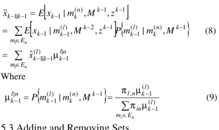
5.2 Initialization of New Models and Filters
The key to the optimal initialization of new models and filters is the concept of state dependency of the system mode set. It simply states that given the current mode (and base state), the set of possible modes at the next time is a subset of the mode space, which is determined by the (Markovian) mode transition law. The optimal assignment of the initial probability to a new model accounts only for the probabilities of those models that may jump (switch) to this new model, and the optimal initial state estimate for a filter based on a (new or old) model is determined only from the estimates (and the probabilities) of the filters based on those models that may jump to the model.
Specifically, the optimal initialization of a filter based on a new (or old) model mn can be done as follows. When
calculating
E
[
x
k|
m
k(n);
M
k1,
~
z
]
, only the previous estimatesx
ˆ
k(l)1|k1 based on models in the setEnshould beused, whereEnis the set of models in Mk1that are allowed to switch tomn:
: 1, , 0
l l k ln
n m m M
E π (7)
n l
n l
E m
n l k l
k k
k n k l k E
m
k k l k k
k k n k k k
k
x
M m m P z M m x E
z M m x E x
| 1 ) (
1 | 1
1 ) ( ) (
1 1 2 ) (
1 1
1 1 ) ( 1 1
| 1
ˆ
, | ,
, |
, , |
µ
(8)
Where
n i E m
l k in
l k n l k
n k l k n l
k Pm m M ()
1 ) (
1 , 1 ) ( ) (
1 |
1 | ,
µ π
µ π
µ (9)
5.3 Adding and Removing Sets
Perform N model-set sequential likelihood ratio test.
HN s MN vs HN s MN
M s H vs M s H
1 1
1 1 0 0
:
,.... :
:
These tests are implemented by using thresholds
β α
1
B and A=-∞ . This step ends when only one of
the hypothesesH1, H2;……,HNremains. Specifically:
Reject set that includes Mi for which
B L
L kM
k M k
i i
/
Continue to the next time cycle to test for the remaining pairs with one more measurement until only one of the hypothesesH1,H2,…..,HN, sayHj,
is not rejected.
5.4 Re-initialization of the off sets
The likelihood functions for filterjis as follows:
) ( ~ ) ( ) ( ~ 2 1 exp ) ( 2
) ( ; 0 ); ( ~ ) (
1 2
1
k z k S k z k
S
k S k z N k
j j T j j
j j j
π (10)
Where z~j(k)z(k)z(k|k1) is the innovation for filterj and
Sj(k)is the covariance matrix.
Switching between active sets as α
j(k) j(k 1) (11)
The model set of
M
j is change to off state and initiate theother two sets.
One Cycle of Switching sets of IMM
Start one cycle for each set of IMM
3 , 2 , 1 ,.... 2 , 1 ) ) ( ( max )
( ,
ki kijwherej andi
For i=1:3
If(k)iβ Set I change to off state
Else active End.
If(k)i(k1)iα
Change the state to off and activate the other sets Else set is active.
End. End.
Compare all i(k) the smallest i(k) takes its highest mode l probability to be the set probability
Set probability of the other two sets=1- probability of minimum
) (k i
If the remaining sets are active
Distribute this value between them according to their maximum model probability. Else
Set the probability of the off sets to zero End.
For active set which has the maximum probability we take its output
i i k i
k k k k k
k Ex z x
x () ()
|
| [ | ] ˆ
ˆ µ
6 The Results of IMM of The First Tracking
Problem
We tested our model using Matlab 2010Ra. intel core 2 duo., under windows vista environment. The following results is for 10 modes one for linear motion and the others
are at differentω [0.2,0.4,0.6,0.8,0.9,1.1,1.4,1.6,1.8],
Q=diagonal(0.52)R=diagonal(100). The results are the average of 200 run. The target trajectory described in
Table1: target trajectory
scenario First trajectory Second trajectory
0<k<90 ω=1.4 ω=1.4
90<k<150 ω=0.2 ω=1.6
150<k<200 linear linear
200<k<300 ω=1.9 ω=1
The transition matrix has a diagonal of 0.82 while all models start with equal model probability
Table 2: The results of the first target trajectory IMM
RMSE x
RMSEy RMSEv x
RMXEvy Value T Exe.time
0.6174 2.9391
0.6039 2.711
0.3242 1.416
0.2970 1.528
Mean Max
2.3 0.01443 0.6275
2.041
0.691 2.9366
0.4422 1.504
0.3774 1.6223
Mean Max
2.5 0.01443 0.7423
3.3473
0.6081 2.4812
0.2973 0.9727
0.3163 1.4287
Mean Max
2.9 0.01440 2 1.0326
4.9509
1.0102 4.509
0.3486 1.2098
0.4908 1.2983
Mean Max
3.3
Table3: the results of the second target trajectory IMM
RMSE x
RMSEy RMSEv x
RMXEvy Value
T
Exe time 0.61742.9391
0.6039 2.711
0.3242 1.416
0.2970 1.528
Mean Max
2.3 0.01443 0.6275
2.041
0.691 2.9366
0.4422 1.504
0.3774 1.6223
Mean Max
2.5 0.01443 0.7423
3.3473
0.6081 2.4812
0.2973 0.9727
0.3163 1.4287
Mean Max
2.9 0.01440 1.0326
4.9509
1.0102 4.509
0.3486 1.2098
0.4908 1.2983
Mean Max
3.3
0.01449 8
7. Hierarchal Switching of IMM
In the above examples we change models with ω near to each other while the change of linear model can take place at anyk. the sudden jump of ω to far values cause system to diverge. Also in this model we choose ω that can introduce good results with each other not all values of them cause system converge or good tracking. Also Not wide range of the time step variation is available.
Two overcome these limitation we introduce a variable set of models. We take the advantage of good tracking of small sets of IMM and divide our structure into three sets The first set includes ω1=[0.2 0.4 0.6] .The second set
includes ω2=[0.8 0.9 1.1]
The third set includes linear model with ω3=[1.4 1.6 1.8]
.The variable structure of IMM algorithm is shown in figure 2
The transition matrix of the first two set and model probability as follow
3 . 0
3 . 0
4 . 0
98 . 0 01 . 0 01 . 0
01 . 0 98 . 0 01 . 0
01 . 0 01 . 0 98 . 0
Pr µ
The transition matrix of the third set has 0.97 diagonal and equal model probability
Fig.2 The Hierarchal structure of IMM for the three sets
8. The results of Hierarchal Structure of IMM
for The First Tracking problem
We tested our model using Matlab Ra2010 on intel core 2 duo., under windows vista environment. The following results is for 10 modes one for linear motion and the others are at different ω [0.2,0.4,0.6,0.8,0.9,1.1,1.4,1.6,1.8],
Q=diagonal(0.52) R=diagonal(100). The results are listed in table 4. The system characterized by unknown changeable structure as in the previous first example.
Table:4 The results of the first tracking problem IMM
RMSEx RMSEy RMSEvx RMXEvy value T Exe. time
2.2637 18.505
3
1.1498 5.039
0.6093 3.6603
0.4307 2.5497
Mean Max
2.3 0.0066
2.6597 7.2371
2.4558 7.3775
1.0951 4.0049
0.9815 4.078
Mean Max
2.5 0.0066 0.6341
5.1443
0.6489 5.034
0.5999 1.8247
0.6096 1.5653
Mean Max
2.9 0.0067 2.5489
7.929
2.7573 7.603
0.8608 3.2303
0.8229 3.0638
Mean Max
3.3 0.0065 3.4279
14.176 2
3.2624 13.3039
1.1856 3.9484
1.2166 3.9018
Mean Max
4 0.0067
2.4515 8.2294
2.6506 9.7918
0.8125 3.1517
0.9002 5.5053
Mean Max
5 0.0065
If we change ω to ω1=[7/dt 8/dt 9/dt] ω2=[4/dt 5/dt 6/dt]
and ω3 =[1/dt 2/dt 3/dt] with linear model. These values
include most of the turning angles that have good separation between modes of operation. The other values included in these modes. The RMSE for the same parameters of the IMM are listed in table 5 while the results of RMSE if we choose R=I 25, are listed in table 6
Table 5: The result of the first tracking problem
HSIMM
RMSEx RMSEy RMSEvx RMSEvy value T Exe time
17.6978 1.8674
18.2421 2.1699
2.2899 0.5395
2.6145 0.5922
Max Mean
2.3 0.0071
7.6344 0.872
12.4231 1.1034
3.0548 0.6205
1.9364 0.4502
Max Mean
2.5 0.0068
10.5143 0.9774
15.9724 1.2805
2.2557 0.4727
1.8583 0.4726
Max Mean
2.9 0.007
15.8625 1.1525
11.5765 1.0396
2.3474 0.4897
2.4372 0.4882
Max Mean
3.3 0.007
13.3789 1.0023
7.4274 0.9793
2.8286 0.9544
2.2394 0.8300
Max Mean
4 0.0067
11.5338 1.6121
14.1307 1.3044
1.814 0.6895
3.4595 0.8429
Max Mean
5 0.0067
Z(k+1)
) 1 | 1 (k k X
)
1 ( 2
) 1 | 1 ( 2
k v
k k X
) 1 ( 1
) 1 | 1 ( 1
k v
k k X
Set 1 IMM1
Set2 IMM3
System )
1 (k v
w(k+1)
) 1 ( 3
) 1 | 1 ( 3
k v
k k X
Switching the
sets ON Or OFF Get right state Set3
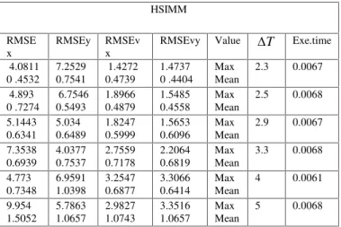
Table 6: The result of the Other sets for the same target trajectory HSIMM
RMSE x
RMSEy RMSEv x
RMSEvy Value T Exe.time 4.0811
0 .4532
7.2529 0.7541
1.4272 0.4739
1.4737 0 .4404
Max Mean
2.3 0.0067
4.893 0 .7274
6.7546 0.5493
1.8966 0.4879
1.5485 0.4558
Max Mean
2.5 0.0068
5.1443 0.6341
5.034 0.6489
1.8247 0.5999
1.5653 0.6096
Max Mean
2.9 0.0067
7.3538 0.6939
4.0377 0.7537
2.7559 0.7178
2.2064 0.6819
Max Mean
3.3 0.0068 4.773
0.7348
6.9591 1.0398
3.2547 0.6877
3.3066 0.6414
Max Mean
4 0.0061
9.954 1.5052
5.7863 1.0657
2.9827 1.0743
3.3516 1.0657
Max Mean
5 0.0068
9. Results of The second Tracking Problem
The target measurement model
)] ( ) ( [ ) ( ) 1
(k Fxk Gak wk
x (12)
,.... 2 , 1 , 0 ); 1 ( ) 1 ( ) 1
(k Hxk vK k
z (13)
Where
x
(
x
,
v
x,
y
,
v
y)
denotes the targets state)
,
(
a
xa
ya
is the acceleration, w~N[0,Q] is theacceleration process noise,
z
(
z
x,
z
y)
is themeasurement, v~N[0,R]is the random measurement error
and
T T T T
G T T
F
0 2 / 0
0 0 2 /
1 0 0 0
1 0 0
0 0 1 0
0 0 1
2 2
The unknown true acceleration is assumed piecewise constant, varying over a given continuous planar regionAc. In the MM framework, we consider a generic finite set
(grid) of acceleration values:Ar
ai Ac i r
,... 2 , 1 : ) ( )
(
which defines the total model set. We approximate the evolution of the true acceleration over the quantized set
A
(r) via a Markov chain model, that is, akA(r) with given
ii P a a
P 0 () and P
a a a a
ij i j r ik i
k | for , 1,2,....
) ( 1 )
(
π .
Consider the following target-tracking example, adopted from [8],[18],[17],[19]. A target moves in the horizontal plane that may have piecewise-constant acceleration with a maximum value of 4g (40m/s2) in any direction. Assume that the following set of 13 time-invariant models, characterized by the expected acceleration vector a, is used:
] 2 , 0 [ 20
] 0 , 2 [ 20 ] 2 , 0 [ 20 ] 0 , 2 [ 20 ] 1 , 1 [ 20
] 1 , 1 [ 20 ] 1 , 1 [ 20 ] 1 , 1 [ 20 ] 1 , 0 [ 20
] 1 , 1 [ 20 ] 1 , 0 [ 20 ] 0 , 1 [ 20 ] 0 , 0 [ 20
13
12 11
10 9
8 7
6 5
4 3
2 1
a
a a
a a
a a
a a
a a
a a
The transition relations among models are easily understood in terms of the directed graph (i.e., digraph) representation of an MM, introduced in [13], [15], [14], [16]. The topology of model set A(13) is depicted in Figure 3. Each model is viewed as a point in the mode (acceleration) space. An arrow from one model to another indicates a legitimate model switch (self-loops are omitted) with non-zero probability.
Fig. 3 Digraph representation of 13-model set
8.1 Design of VIMM and HSIMM
For both VIMM and HSIMM we divide the sets into three sets. M1{a2,a3,a11,a6,a10} , M2{a9,a5,a13,a8} and
} , , ,
{1 4 7 12
3 a a a a M
The probability transition matrix of IMM13 and VIMM has diagonal of 0,8
The model probability is
0.08 0.08 0.08 0.076 0.076 0.076 0.076 0.076 0.076 0.076 0.076 0.076 0.076
µ
For HVSIMM we have three sets each set has its own transition matrix and model probability as follow
Set1
8 . 0 04 . 0 04 . 0 04 . 0 04 . 0
04 . 0 8 . 0 04 . 0 04 . 0 04 . 0
04 . 0 04 . 0 8 . 0 04 . 0 04 . 0
04 . 0 04 . 0 04 . 0 8 . 0 04 . 0
04 . 0 04 . 0 04 . 0 04 . 0 8 . 0
π µ
0.2 0.2 0.2 0.2 0.2
97 . 0 01 . 0 01 . 0 01 . 0
01 . 0 97 . 0 01 . 0 01 . 0
01 . 0 01 . 0 97 . 0 01 . 0
01 . 0 01 . 0 01 . 0 97 . 0
π µ
0.25 0.25 0.25 0.25
The sets probability is initialized by
0.4 0.3 0.3
Set
µ . It is changed according to the maximum model probability of the model of sets. The active set takes higher value while the other is distributed according to their higher model probability.
8.2 Performance Evaluation
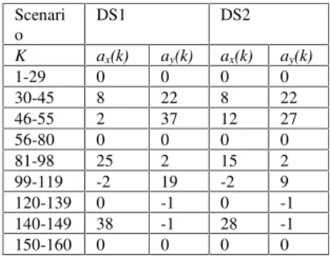
Test scenarios
The performances of the IMM, VIMM and HSIMM tracking algorithms were investigated first over a large number of deterministic maneuver scenarios with fixed acceleration sequences. Deterministic scenarios serve to evaluate algorithms’ peak errors, steady-state errors and response times. We present two of them, referred to as DS1 and DS2, in the sequel. Their acceleration values are given in Table 7
Deterministic Scenarios’ Parameters
The other parameters for both scenarios areT = 1s; Q =
O; R =1250I; x0= [8000; 25; 8000; 200]. Note that while
the acceleration values in DS1 are relatively close to the fixed grid points of IMM13, in DS2 they are deliberately chosen far apart from the grid points. As such, for the fixed structure estimator IMM13 the scenario DS2 is more difficult than DS1.
Table 7: The Targets Dynamics
Performance measure:
Theaccuracyof the algorithms was measured in terms of
position and velocity root-mean-square errors (RMSE):
T j M
j
j k xk x k x
k x M k error
RMS_ ( ) 1 ( ( ) ( ))(( ) ( )
1
21 1
| |
2 1 1
| |
ˆ * ˆ 1
RMSE
ˆ * ˆ 1
RMSE
M
i
i k k i k i
k k i k y
k M
i
i k k i k i
k k i k x
k
y y y y M
x x x x M
,
21 1
2 | 2
|
2 1 1
2 | 2 |
ˆ ˆ
1 RMSE
ˆ ˆ
1 RMSE
M
i
i k k i k i
k k i k vy
k M
i
i k k i k i
k k i k vx
k
y y y y M
x x x x M
Where
ik i k i
k i k i
k i k i
k i
k y x y x y x y
x , trueposition, , true velocity,ˆ ,ˆ estimatedpositionˆ ,ˆ
and the estimated velocity.
The performances of the three MM tracking algorithms are investigated first over a large number of deterministic maneuver scenarios with fixed acceleration sequences. Deterministic scenarios serve to evaluate algorithms’ peak errors, steady-state errors and response times. We present two of them, referred to as DS1 and DS2, in the sequel. Their acceleration values are given in Table 7. The other parameters for both scenarios areT=1 sec, Q=0,R=1250I
Note that while the acceleration values in DS1 are relatively close to the fixed grid points of IMM13, in DS2 they are deliberately chosen far apart from the grid points. As such, for the fixed structure estimator IMM13 the scenario DS2 is more difficult than DS1.
Table 8: The results of target dynamics in table 7
IMM13 VIMM13 HSIMM13
DS1 DS2 DS1 DS2 DS1 DS2
RMSx 0.0182 0.0118 0.0.094 0.0892 5.6850 4.2039 RMSy 0.0291 0.0276 0.312 0.3131 3.6809 5.6190 RMSvx 103.309
2
74.822 4
105.635 1
75.133 0
23.876 4
16.058 0 RMXvy 97.7809 93.333
6
103.902 3
99.936 8
15.207 6
10.526 1
Table 9: The execution Time of target dynamics in table 7
IMM13 VIMM13 HSIMM
DS1 DS2 DS1 DS2 DS1 DS2
Time 0.0.007 5
0.0072 0.0085 0.0073 0.0045 0.0019 Scenari
o
DS1 DS2
K ax(k) ay(k) ax(k) ay(k)
1-29 0 0 0 0
30-45 8 22 8 22
46-55 2 37 12 27
56-80 0 0 0 0
81-98 25 2 15 2
99-119 -2 19 -2 9
120-139 0 -1 0 -1
140-149 38 -1 28 -1
0 20 40 60 80 100 120 140 160 0
0.1 0.2 0.3 0.4 0.5 0.6 0.7 0.8 0.9 1
Time
s
e
t
p
ro
b
a
b
il
it
y
set1 set2 set3
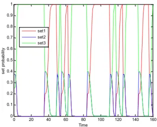
Figure 4 Activation between the sets as their set probability change for DS1 of HSIMM13
0 20 40 60 80 100 120 140 160 0
0.1 0.2 0.3 0.4 0.5 0.6 0.7 0.8 0.9 1
time
se
t
pr
ob
ab
ili
ty set1
set2 set3
Figure 5 Activation between the sets as their set probability change for DS2 of HSIMM13
The proposed HSIMM introduced less computational time and also minimum RMS error as shown in table 5, 6,8 and 9. But it needs to be re-initialized to overcome error accumulation.
The activation between included sets is achieved by the introduced threshold value of innovation. The switching algorithm as shown in figure 4 and 5 for DS1 and DS2 is effective.
10. Conclusion
As the number of the IMM increase the algorithm stability decrease. Or in other word As the parameters change the system doesn’t converge to different values. As we show in IMM with 10 models. The change ofωandT . Also the choosing of their values may cause system to converge to the wrong model of ω. Also as the time step change the (increase) the system doesn’t converge as ω and time step change together. Not all the models change during operating from model to another allowed.
In structure set of IMM we first choose the near values of ω in the same model to avoid converging to the wrong set. The small numbers of models increase the system stability. Itdoesn’t diverge at the changing of time step or different values of ω. Also changing from any model to another is allowed. The advantages of the structure set of IMM are introducing varieties of motion models and also varieties of time step values. Introduce variety of Model change during operation. Introduce large number of modes of operation so we can avoid using the nonlinear models with their calibration hardness. It also introduce less computation time than introduced by the large number of IMM since we only activate the right set.
The error introduced by the structure HSIMM is due to the initialization at the beginning before converging to the right set. This error can be reduced by the refinement process if we take the saved values of the right set but it doesn’t suite the real time process. The HSIMM also introduce relatively similar errors at velocity components compared to other algorithms. The computational time is minimum than introduced by IMM and VIMM. HSIMM introduces less error as the noise increase and there is no need for re adjustment to the Covariance as the noise increase so it is more robust against noise and introduces minimum computational time.
References
[1] E. Mazor, A. Averbuch, Y. Bar-Shalom, and J. Dayan. Interacting multiple model methods in target tracking: A survey. IEEE Transactions on Aerospace and Electronic systems, 34(1):103{123, January 1998.
[2] X.R. Li and Y. Bar-Shalom. Multiple-model estimation with variable structure. IEEE Transactions on Automatic Control, 41(4):478{493, April 1996.
[3] Hongshe Dang, Chongzhao Han Xi’an, Shaan and Dominique GRUYER “Combining of IMM filtering andDS data association for multi-target tracking” www.fusion2004.foi.se/papers/IF04-0876.pdf
[4] Ludmila Mihaylova and Emil Semerdjiev, “An Interacting Multiple Model Algorithm for Stochastic Systems Control” www.citeulike.org/user/sourada/article/347493 - 16k [5] Leigh A. Johnston and Vikram Krishnamurthy, “An
Improvement to the Interacting Multiple Model (IMM) Algorithm, IEEE TRANSACTIONS ON SIGNAL PROCESSING, VOL. 49, NO. 12, DECEMBER 2001 PP 2909-2923.
[6] Joseph J. LaViola Jr. “A Comparison of Unscented and Extended Kalman Filtering for Estimating Quaternion Motion”.
www.cs.brown.edu/people/jjl/pubs/laviola_acc2003.pdf -[7] Songhwai Oh and Shankar Sastry, ”An Efficient Algorithm
for Tracking Multiple Maneuvering Targets”. Proc. of the IEEE International Conference on Decision and Control, Seville, Spain, Dec. 2005.
by IMM Estimator.
http://citeseer.ist.psu.edu/cache/papers/cs/22073/
[9] Youmin Zhang and X. Rong Li., “Detection and Diagnosis of sensor and actuator failures using IMM estimator”, IEEE TRANSACTIONS ON AEROSPACE AND ELECTRONIC SYSTEMS .vol.34, No. 4 October 1998. PP 1293-1313. [10] Donka Angelova 1 , Emil Semerdjiev 1 , Ludmila
Mihaylova 1 X. Rong Li , “An IMMPDAF Solution to Benchmark Problem for Tracking in Clutter and Standoff Jammer”,http://citeseer.ifi.unizh.ch/cache/papers/cs/22073/ [11] Simon J. Julier Jeffrey K. Uhlmann,”A New Extension of
the Kalman Filter to Nonlinear Systems”. media/pdf/Julier1997_SPIE_KF.pdf/kalmanwww.cs.unc.ed u/~welch/
[12] Seham Meawed Aly , Raafat El Fouly, Hoda Barak, “Extended Kalman filtering and interactive multiple model for tracking maneuvering targets in sensor networks,” Intelligent solutions in embedded systems,2009 seventh workshop on, 2009 , page: 149-156
[13] X. R. Li, V. P. Jilkov, and J.-F. Ru, “Multiple-model estimation with variable structure—part VI: expected-mode augmentation,” IEEE Transactions on Aerospace and Electronic Systems, 41(3): 853–867, July 2005
[14] X. R. Li, Z.-L. Zhao, and X. B. Li, “General model-set design methods for multiple-model approach,” IEEE Transactions on Automatic Control, 50(9):1260–1276, September 2005
[15] X. R. Li, "Engineer's guide to variable-structure multiple-model estimation for tracking," Y. Bar-Shalom and W. D. Blair, eds., Multitarget-Multisensor Tracking: Applications and Advances, Vol. 3, Chapter 10, Artech House, Boston, 2000, pp. 499-567 [16] Xiao-Rong-Li, Yaakov Bar-Shalom, “Multiple- Model Estimation
with Variable Structure “ ,IEEE Transactions on Automatic Control, Vol. 41, No, 4 April 1996. pp.478-493.
[17] X. R. Li, "Engineer's guide to variable-structure multiple-model estimation for tracking," Y. Bar-Shalom and W. D. Blair, eds., Multitarget-Multisensor Tracking: Applications and Advances, Vol. 3, Chapter 10, Artech House, Boston, 2000, pp. 499-567 [18] X. R. Li, and Y. M. Zhang, “Multiple-Model Estimation With
Variable Structure—Part V: Likely-Model Set Algorithm,”IEEE Trans. Aerospace and Electronic Systems, Vol. AES-36, Apr. 2000.