www.atmos-meas-tech.net/8/2685/2015/ doi:10.5194/amt-8-2685-2015
© Author(s) 2015. CC Attribution 3.0 License.
Impacts of atmospheric state uncertainty on O
2
measurement
requirements for the ASCENDS mission
S. Crowell1, P. Rayner2, S. Zaccheo3, and B. Moore1
1School of Meteorology, University of Oklahoma, 100 David Boren Blvd, Norman, OK 73072, USA 2School of Earth Sciences, University of Melbourne, Melbourne, Australia
3Atmospheric and Environmental Research, 131 Hartwell Avenue, Lexington, MA 02421, USA
Correspondence to:S. Crowell ([email protected])
Received: 16 May 2014 – Published in Atmos. Meas. Tech. Discuss.: 10 July 2014 Revised: 05 June 2015 – Accepted: 08 June 2015 – Published: 03 July 2015
Abstract. Remotely sensed observations of atmospheric composition require an estimate of surface pressure. This es-timate can either come from an instrument with sensitivity in an O2absorption feature in the spectrum, or it can be
pro-vided by a numerical weather prediction (NWP) model. In this work, the authors outline an information-based method-ology for setting measurement requirements for an active li-dar measurement of O2in the context of the Active Sensing
of Carbon Emissions over Nights, Days and Seasons (AS-CENDS) mission. The results indicate that the impacts of correlations in the environmentally induced vertical weight-ing function errors between CO2and O2measurements are
nontrivial and that the choice of CO2and O2wavelengths can
lead to a stricter or looser requirement than that of surface pressure considerations alone, which would indicate about a 0.1 % precision for 1mb accuracy. Furthermore, the less sen-sitive the CO2measurement is to surface pressure errors, the
more difficult it will be for an O2 observation to provide a
useful measurement.
1 Introduction
The present surface-based network of observing systems has been shown to be inadequate for reducing uncertainty in sur-face flux estimates of CO2at all but the coarsest spatial scales
(Houweling et al., 2004). However, other experiments with pseudo-data (e.g., Rayner and O’Brien, 2001; Houweling et al., 2004; Hungershoefer et al., 2010) suggest that column-integrated CO2mixing ratio, denoted as XCO2, as retrieved
from radiances measured by satellites with instruments that
are sensitive to CO2absorption features, can provide enough
observations with suitable precision to both improve current surface flux estimates and reduce their associated uncertain-ties. The Active Sensing of CO2Emissions over Nights, Days
and Seasons (ASCENDS) mission will make CO2
measure-ments with high precision and low bias (ASCENDS Work-shop Report, 2008) in order to provide retrievals of XCO2
with errors in the 1–2 ppm range, which is thought necessary to constrain global sources and sinks at the regional scale (Miller et al., 2007).
Satellites measure the top-of-atmosphere radiance, which is sensitive to the integrated amount of absorbing tracer along the photon path. This amount may change with either changes in mixing ratio or of the mass of air through which photons pass. Source–sink processes only change mixing ra-tio. Thus, for best use in flux inversions, retrievals of XCO2
require an estimate of surface pressurep∗to convert the gas number density of CO2 in the column to a dry air mixing
ratio. Two options have been proposed for providing thep∗
estimate for ASCENDS, for which the CO2column number
density would be retrieved using a laser differential absorp-tion spectrometer (LAS). The first is to use the collocated value of surface pressure derived from numerical weather prediction (NWP) models. The second, and more expensive, is to employ a LAS to measure absorption in an O2 band
and utilize the near-constant O2mixing ratio to retrieve a
measure-ments of O2lag the current state of the art for CO2(James
Abshire, personal communication, 2014). The authors note that this need for a surface pressure estimate is not unique to active measurements. Both GOSAT and OCO-2 have detec-tors in O2absorption bands, and these are used to some
ex-tent to retrieve surface pressure, although they are also used for cloud and aerosol screening (e.g., Taylor et al., 2012).
In Zaccheo et al. (2014), the authors set out to quantify the impact of atmospheric state variables, such as tempera-ture (T), relative humidity (RH) and surface pressure (p∗) on retrievals of XCO2. This was accomplished by comparing
weather model forecasts to collocated surface and upper-air observations and using the Line-By-Line Radiative Transfer Model (LBLRTM; Clough et al., 2005) to compute the dif-ferences in optical depth (OD) arising from the different es-timates ofT, RH andp∗, treated as noise, as well as from perturbations to the CO2profile and to the surface pressure
for the O2measurement, which were treated as signal. The
signal and noise were computed for a wide range of different absorption lines, with the conclusion that atmospheric state uncertainties propagate to at least 0.2 ppm addition to the XCO2uncertainty budget, though these numbers are highly
variable depending on the lines selected.
In this paper, we present a methodology to partially answer the question of cost versus benefit for an active O2
measure-ment by determining whether the observations of CO2
mix-ing ratio with the active O2measurement contain more
infor-mation than the NWP prediction on themodel profileof CO2,
denotedqCO2(p), and hence the most information on the sur-face fluxes in a transport model inversion. Specifically, we seek to provide an upper bound on the signal-to-noise ratio (SNR) of the O2measurement, beyond which the cost of the
measurement would not be justifiable. In this work, we uti-lize some of the analysis in Zaccheo et al. (2014), including the matched pairs ofT, RH andp∗to compute the error stan-dard deviations for those quantities and to include those un-certainties in computations of information content for obser-vations with and without an active O2 measurement. There
are a few key differences between this work and that Zaccheo et al. (2014), though they are addressing related questions. First, we are interested in the contribution of an O2lidar but
only relative to the scenario in which no such lidar is flown. That is, we are not attempting to provide estimates of errors in XCO2that arise from each of these scenarios. Secondly,
we do not compute XCO2 explicitly, as it introduces extra
uncertainty into the problem through division by quantities that are uncertain, such as the differential absorption cross section and specific humidity. Thirdly, our method utilizes analytic expressions for the derivatives of various quantities rather than the perturbation method utilized in Zaccheo et al. (2014), which allows us to perform our analysis for many error scenarios and reference states. In principle, this analy-sis could be carried out similarly for any collocated observa-tions.
The paper is laid out as follows. Section 2 defines the ob-servations of interest and relevant terminology. In Sect. 3, the notion of Fisher information is introduced, and the relevant form used in our methodology is discussed. The error com-ponents are defined in Sect. 4. These errors, together with the derivative of the observation operators with respect to theqCO2 in each model layer, are used to calculate the infor-mation in each observation as functions of a few parameters related to observational errors and NWP model surface pres-sure errors. A SNR (precision) requirement for the usefulness of an O2measurement is derived in Sect. 3.4 and computed
in Sect. 5 for the O2error for different magnitudes of surface
pressure error.
2 Differential absorption lidar measurements
LAS instruments measure the difference in transmit-ted/received energies at two or more wavelengths (which for the two-line case we call “Ton” and “Toff”).Tonis
transmis-sion on a wavelength absorbed by CO2whileToffis on a line
not subject to absorption by CO2. We denote the logarithm
of the ratio as1τ, the differential optical depth (DOD). That is,
1τCO2:= −log T
on Toff
=
p∗ Z
0
qCO2(p)1ξCO2(p) mdg(p)(1+qH2O(p)
mH20
md )
dp, (1)
where md is the molecular mass of dry air, mH2O is the molecular mass of water,qH2O(p)is the dry air mixing ra-tio of water,gis gravitational acceleration and1ξCO2 is the differential absorption cross section at pressure altitude p. This definition follows immediately from Beer’s Law, which states that the transmission is given by
T =exp −
R2 Z
R1
ngas(r)ξgas(r)dr
,
withngas being the number density of the gas andr denot-ing the path traversed by the laser. Note that we could refor-mulate these definitions in terms of geometric heightzin the case that this is more convenient, since the lidar also provides this measurement through ranging. Since the actual quanti-ties measured by the instrument areTonandToff, the quantity 1τCO2 is the most direct link between the actual observation and the model profileqCO2(p), assuming thatp
∗and1ξ
CO2 are known. The derivative of1τCO2 (or1τO2) per unitqCO2 (qO2) as a function of the vertical coordinate (herep) will be referred to as the vertical weighting function (WF):
W×(p)=
1ξ×(p)
mdg(p)(1+qH2O(p)
mH20
md )
where × is either CO2 or O2. This function tells us what
portion of the vertical column is providing the most weight to the retrieval of column integrated CO2or O2. From Eq. (1)
we can see that the WF is just1ξCO2or1ξO2normalized by mdandg.
The observation operator maps the model state (qCO2) into the space where the observations lie. The candidate observa-tions in this document are the differential optical depth for CO2(using NWPp∗),1τCO2, given in Eq. (1), and the ratio
1τCO2
1τO2 , which is written explicitly as
1τCO2 1τO2
= Rp∗
0 qCO2(p)WCO2(p) Rp∗
0 qO2WO2(p)dp
. (3)
Note that the ratio 1τ1τCO2
O2 resembles (modulo the different WFs) the ratio qqCO2
O2 and so can be thought of as a surrogate for XCO2, with appropriate scaling for the abundance of O2
in the atmosphere. XCO2is not considered explicitly in this
treatment, because it is not directly tied to the quantities mea-sured or to the model profile of mixing ratio. In practice, in-verse calculations ingest XCO2, and we assume that the total
information on model mixing ratio is the same whether we ingest the direct measurements of differential optical depth (with an online computation forW) or retrieve XCO2andW
offline and ingest them separately.
For ASCENDS, three candidate spectral lines have been identified as having the most potential for estimating absorp-tion due to CO2(ASCENDS Workshop Report (2008)): two
lines in the weak CO2band near 1.571 and 1.572 µm and the
strong CO2 band near 2.06 µm. To accompany these
mea-surements and convert them to XCO2, two oxygen
measure-ments have been proposed: one in the oxygen A band near 0.76 µm and the other near 1.26 µm (ASCENDS Workshop Report, 2008).
The online and offline wavelengths are chosen with con-sideration of the sensitivity of transmission to atmospheric temperature, water vapor and pressure, since variability in these quantities will contribute to the overall uncertainty in the retrieved gas number densities. For example, Abshire et al. (2014) and Riris et al. (2013) specify the interest in the 1.572 and 0.76 µm region for CO2and O2, respectively,
for decreased sensitivity in absorption to temperature fluctu-ations.
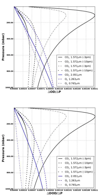
Figure 2, which is described in greater detail in Sect. 4.2.2, shows typical vertical WFs for these spectral lines for few different choices of online wavelength. By specifying a dif-ferent offset (3 or 10 pm), the layer of the atmosphere to which the measurement is most sensitive is varied. The value of1τCO2arising from the 1.571 µm–3 pm online wavelength is more indicative of the composition near the top of the tro-posphere, because the online wavelength is closer to line cen-ter than that of the 10 pm offset, which peaks closer to the surface. The 2.051 µm 1τCO2 is more indicative of values
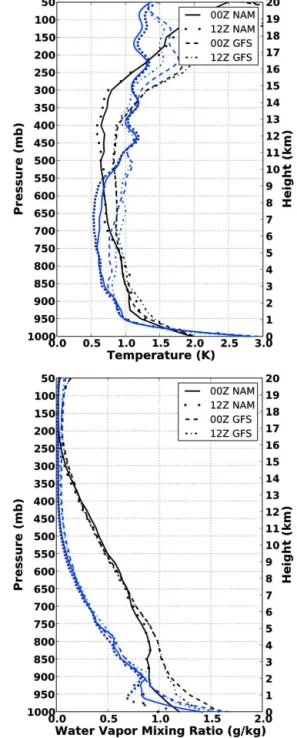
Figure 1.From Zaccheo et al. (2014). Ensemble RMS differences between RAOB measurements and corresponding NWP analysis temperature (top) and water vapor mixing ratio (bottom) profiles. Each panel illustrates the errors for 0Z and 12Z NWP analysis fields, respectively. The black lines represent the respective RMS differences as a function of pressure and the blue lines denote the RMS as a function of vertical height from the surface.
near the surface due to the stronger absorption in the strong CO2band that allows an online wavelength further from the
3 Information content
From (Rodgers, 2000), the Fisher information for the lin-earized retrieval problem with Gaussian error statistics is given by
I=HTR−1H+B−1, (4)
whereRis the observation error covariance matrix,Bis the prior error covariance matrix and His the Jacobian of the observation operatorhthat transforms model variables into observations. The Fisher information can be thought of as the information in the observation or retrieval about the input parameters, which compose the domain ofh, and is simply the inverse of the posterior error covariance matrix.
For the observation operators in Eqs. (1–3), the predicted quantity is a scalarh, meaning that its gradient (with respect to each variable) His a column vector. Assuming that the prior information onqCO2 is the same for each candidate ob-servable (i.e., they assume the same error statistics), this sug-gests that the scalar quantity
IqCO2 =HTqCO2R−1HqCO2 (5)
provides a measure of a particular observable’s information content on the model profile of CO2. Here,HqCO2 is the
Jaco-bian (or gradient) ofhwith respect to thenlayersmodel layer
mixing ratios[qCO1 2, . . ., q
nlayers
CO2 ], and so the quantity q
IqCO2
has units ppm−1regardless of the units ofh. This quantity thus provides a useful manner in which to compare the util-ity of very different observations. It should be noted that the JacobianHqCO2 is expensive to estimate for passive
measure-ments (e.g., using a finite difference approximation) but is quite simple to compute analytically in the case of a lidar measurement, by simply differentiating Eqs. (A1) and (A2) (the discrete versions of Eqs. (1) and (3) with respect to the layer mixing ratiosqCOi
2) to yield Eqs. (A3) and (A4). It re-mains to computeR, which is described in detail in Sect. 4.
IqCO2 combines the effects of the sensitivity (i.e., the
derivative) of an observation toqCO2 with noise (i.e., the er-ror statistics encapsulated inR). In this way, by usingIqCO2
as a metric we follow a balanced approach to decide the most useful error requirements.
3.1 Sources of error
For a linear retrieval, the matrix Rcharacterizes the uncer-tainty present in the model’s predicted value of the observa-tion as well as the observed value itself (Tarantola, 2005). As such,Ris a combination of instrument precision (i.e., signal to noise), the uncertainty in the simulated/retrieved external quantities (such as surface pressure, temperature and mois-ture) and the uncertainty from things that are not explicitly modeled, such as errors in spectroscopy. The first source is treated as random error with known statistics computed from the signal-to-noise ratios. The second source includes surface
pressure errors and errors in the calculated WF (1ξCO2) due to misspecification of local temperature and water vapor, on which the WF calculation strongly depends. The third cate-gory of errors is assumed to be negligible since we assume that transmission in nearby wavenumbers differs only in the gas absorption, and so all other effects vanish when we take the difference. This is the typical assumption for DIAL-type instruments and indeed the inspiration for the DIAL concept. Assuming a single sounding in the retrieval (or spa-tially uncorrelated errors),Ris a constantσ2(h), and hence
IqCO2= |H|2σ−2(h). The variance σ2(h) is decomposed
based on the considerations in the previous paragraph as
σ2(h)=σp2∗(h)+σ1ξ2 (h)+σobs2 (h), (6) wherehis either1τCO2 or
1τCO2
1τO2 . Thehdependence is
in-cluded to emphasize the variability of the observationhdue to errors in surface pressure, the weighting function (aris-ing from errors in temperature and humidity) and instrument noise. Thus the information in a single measurement on the co-located modelqCO2 is σ
−2(h)|H
qCO2|2, which suggests
that theith component ofσ−1(h)HqCO2 will represent the
in-formation in the observable about the model’sith layer CO2
mixing ratio.
In Sects. 4.2 and 4.3 we make use of the uncertainty prop-agation formula, which says that ify=h(x) andH= ∇h, then
Ry=HTRxH, (7)
whereRx and Ry are the covariance matrices of x andy,
respectively. We use it here to connect the uncertainties in the ratio1τ1τCO2
O2 to1τCO2and1τO2, the error variances of which are given by Eq. (6). The details of these calculations for the atmospheric state induced errors are discussed in Sect. 4. 3.2 The observational error varianceσ2
obs(h)
The observed differential absorptions1τ contain an instru-ment specific level of precision, controlled by the laser power and detector sensitivity, which we refer to asσobs2 (h). This is typically quantified by the lab that builds and tests the instru-ment in a controlled environinstru-ment. The ratio observable has “noise” defined as the propagation of the noise from the CO2
and O2 instruments (assuming no correlations between the
two DOD measurement errors):
σobs2
1τCO2 1τO2
=1τO−2 2σ
2
obs(1τCO2)
+1τCO2 21τ
−4 O2σ
2
obs(1τO2). (8)
other, keeping the error budget for XCO2fixed. However,
in-creasing precision has an added cost (e.g., associated with increasing laser power or developing more sensitive detec-tors) which cannot be left out of cost–benefit analyses used in decision making.
3.3 The total error variance for1τCO2 and 1τCO2
1τO2 In order to compute the information in each observation we summarize the preceding subsections in terms of expressions for the total uncertainty in each observation, which is just the sum of the three components described at length above.
For 1τCO2, assuming an estimate of p
∗ from a NWP model, and using the expressions Eqs. (A5) and (A7), we have
σ2(1τCO2)=σp2∗(1τCO2)+σ1ξ2 (1τCO2)+σobs2 (1τCO2), =(qCO1
2W 1 CO2)
2σ2
NWP(p∗)+
+ ∇WCO2(1τCO2)
TR
1ξCO2∇WCO2(1τCO2)+
+σobs2 (1τCO2), (9)
where∇WCO2(1τCO2)is a vector of lengthnlayerswhose en-tries are given by Eq. (A7).
Similarly, for 1τ1τCO2
O2 we use the expressions Eqs. (A6), (A8) and (A9) to define
σ2
1τ
CO2 1τO2
=σp2∗
1τ
CO2 1τO2
+σ1ξ2
1τ
CO2 1τO2
+
+σobs2
1τCO2 1τO2 , =
qCO1 2W
1 CO2 1τO2
−1τCO2
1τO2 2
qO1 2W
1
O2 !2
σNWP2 (p∗)+
+ ∇W
1τ
CO2 1τO2
T R1ξ∇W
1τ
CO2 1τO2
+ (10)
+1τO−2 2σ
2
obs(1τCO2)+1τ 2 CO21τ
−4 O2σ
2
obs(1τO2),
where∇W
1τ CO2
1τO2
is a vector of length 2×nlayers, whose
entries are derived from Eqs. (A8) and (A9). 3.4 An information-based O2requirement
In Sect. 4, the process of computing scalar error statistics
σ2(h)for1τCO2 and
1τCO2
1τO2 , which assumes no correlations
between the from errors in temperature, water vapor and pressure is described. In the case of differential absorption lidar observables, we have simple analytical expressions for
h, assuming knowledge of the surface pressurep∗ and the weighting function, and so the Jacobian HqCO2 can be
cal-culated directly using Eqs. (A3) and (A4). Using these two pieces, we can computeIqCO2 for1τCO2 and
1τCO2 1τO2 .
A minimum requirement for the O2lidar investment to be
cost effective is that the information in the ratio observable in Eq. (3) is greater than the CO2-only observation, stated as
∇qCO21τCO2
2
σ2(1τCO 2)
≤ ∇qCO2
1τCO2 1τO2 2
σ21τCO2
1τO2
. (11)
Noting that ∂1τCO2
∂qi
CO2
= 1τO2 2
∂ ∂qi
CO2
1τCO2
1τO2 yields the
require-ment
σ2
1τ
CO2 1τO2
≤σ
2(1τ CO2) 1τO2
2
. (12)
Expanding the error variances using Eqs. (9) and (10) and solving forσobs(1τO2), we arrive at
σobs2 (1τO2) 1τO2
2 ≤σ
2
1ξ(1τCO2) 1τCO2
2 −
σ1ξ2 1τ1τCO2 O2 1τ CO2 1τO2 2 + +σ 2
p∗(1τCO2) 1τCO2
2 −
σp2∗ 1τ CO2 1τO2 1τ CO2 1τO2
2 . (13)
Note the lack of the observational error term for1τCO2 on the right-hand side of Eq. (13), meaning that the O2 upper
bound for usefulness isindependent of CO2precision. Also
note that this quantity will only be meaningful if
σ1ξ2 (1τCO2)+σp2∗(1τCO2) σ1ξ2
1τ CO2
1τO2
+σp2∗
1τ CO2
1τO2
≥1τ
2
O2, (14)
which says that the ratio of the errors between the 1τCO2
and 1τ1τCO2
O2 must be greater than the O2 signal. Otherwise, the right-hand side of Eq. (13) would be negative, and so no SNR would yield a useful O2measurement due to one of the
sources of error in the ratio measurement being too large. For a given choice of CO2and O2lines, the right-hand side
of Eq. (13) depends solely on the expected error in surface pressure that arises from using an NWP estimate of p∗ in place of the true value, denotedσ2(p∗).
4 Uncertainty quantification for ASCENDS instrument concepts
In the following subsections, we outline the procedure for computing the uncertainties in the observations1τCO2 and
1τCO2
1τO2 for wavenumbers that are of interest to ASCENDS.
These uncertainties are then used in Sect. 5 to seek viable O2lidar candidates that can add to the information on model
CO2to better constrain flux inversions. Throughout we will
use the notion of relative uncertainty that uses the rela-tion Eq. (12) to suggest that we compareσ(2·)(1τCO2) and
1τO2 2σ 2 (·) 1τ CO2 1τO2
4.1 Observed and NWP-predicted variables
Atmospheric state uncertainties were computed from an extensive set of observation and model prediction pairs derived from surface weather observation station reports (METAR/SYNOP) (US DOC/NOAA OFCM, 2005) and NWP model fields collected both over the continental United States of America as well as on a global basis for representa-tive periods between July 2011 and July 2012. The represen-tative time periods were chosen to include data from all sea-sons as well as both daytime and nighttime observations. The surface observations were obtained from publicly available sources and the matching model data were extracted from both the 12 km North American Mesoscale model (NAM) (Rogers et al., 2009) and 0.5◦Global Forecast System (GFS) (NCEP, 2003) analysis fields. The NAM was chosen to rep-resent the uncertainty statistics associated with a high spatial resolution model for a well-instrumented area, and the GFS fields were chosen to illustrate the errors associated with a coarser global domain. Only 0-hour forecasts or model anal-ysis fields were selected in this work to describe the model error characteristics based on the assumption that any oper-ational retrieval system would either acquire data from an external source or employ an N-dimensional variational data assimilation system to minimize the impact due to uncertain-ties in the atmospheric state. While METAR and SYNOP are by no means an absolute representation of the atmospheric state at any point (Sun et al., 2010), they do provide a consis-tent measure that can be compared to NWP data for statistical purposes.
4.2 The environmental uncertainty contribution
σ2
1ξ(h)
The differential absorption cross section1ξ is a function of the atmospheric state variables, and as such the WFs in an au-tomated retrieval will be dynamically estimated according to local temperature (T), water vapor (Q) and pressure (P). The atmospheric values ofT,QandP will themselves be esti-mates, taken from NWP models, satellite soundings or other proxies. In order to quantify the uncertainty in the observable due to uncertainty in1ξ,σ1ξ(h), the uncertainty in1ξ due
to uncertainty in the atmospheric state must be quantified. This analysis was carried out in a different way in Zaccheo et al. (2014), and we summarize the common methods here. The major difference is that in this work the uncertainties are propagated analytically using derivatives of the lidar obser-vation operators, while in Zaccheo et al. (2014), the sensi-tivities are computed numerically using perturbations. These values should be roughly equal, but our interest lies in de-riving an upper bound for O2SNR to provide a useful
mea-surement, which is why we carry out our computations using analytic derivatives.
Sample sets of simulated absorption cross section for representative CO2 absorption features at 1.571, 1.572
and 2.051 µm and O2 absorption features at 0.76473 and
1.2625 µm were constructed from observed and modeled at-mospheric profile data using the LBLRTM (Clough et al., 2005). The online absorption cross section values were com-puted for CO2at 1.571 and 1.572 µm lines with 3 and 10 pm
offsets and at 2.0510 µm, at the wavenumbers currently be-ing investigated by the ASCENDS instrument development teams. For O2, the online wavelengths chosen were 0.76473
and 1.2625 µm. The offline wavelengths were chosen in a nearby region with similar characteristics for aerosols and atmospheric state variables but reduced sensitivity to absorp-tion by CO2 or O2, so that the difference (1τ) is
predomi-nantly the signal due to the trace gas of interest. Specifically, the offline value chosen was 50 pm off the absorption fea-ture for both weak CO2 lines and the 1.2625 O2 line and
100 pm off the absorption feature for the strong CO2 line
and the 0.76473 O2line. These offline wavelengths were
se-lected from a range of values from 3 to 100 pm and were picked to minimize the difference between the online opti-cal depth and the differential optiopti-cal depth. The upper panel in Fig. 2 shows the WF for the online wavelength OD and the lower panel shows the WF for 1τCO2. The instrument WFs are qualitatively unchanged by subtracting the offline contribution, which is due to the low absorption in the offline wavelength, leading to a flat WF. SinceIqCO2is the derivative
divided by the variability, and this loss of magnitude is expe-rienced by all realizations of the 0.76 µm WF, this difference will effectively cancel out for the purposes of computing in-formation content.
In order to computeσ1ξ(h), which we emphasize is the
expected error in differential absorption cross sectiondue to misspecification of the atmospheric staterather than errors in the spectroscopic characterizations of the bands of inter-est, we computed absorption cross sections with observed and model-predicted values of T, Q and P (described in more detail in the next paragraph) for the online and offline wavenumbersξon andξoff. The differential absorption cross
section1ξ=ξon−ξoff. Since the vertical profiles of1ξ are
being compared for both CO2and O2, the uncertainty in the
absorption cross section for an atmospheric column is most completely described by a covariance matrixR1ξ with
di-mensions(2nlayers×2nlayers), which includes potential cor-relations between errors in the WFs for CO2and O2. We also
point out that though we compute the covariance between errors inT andQ, we assume that errors between these vari-ables and surface pressure errors are uncorrelated. Also, we assume that using pressure as the vertical coordinate forT
andQwill account for any correlations between errors inT
andQand the layer pressure itself. 4.2.1 Compilation ofT andQerrors
mois-ture. The observed profiles were derived from RAwinsonde OBservation (RAOB) observations, while model data were taken from NWP model fields. The RAOBs were obtained from publicly available sources and the matching model data were extracted from GFS (NCEP, 2003) analysis fields. RAOBs provide a consistent measure that can be compared to NWP data for statistical purposes (Sun et al., 2010). The matching NWP profiles were selected using a nearest neigh-bor approach based on the RAOB station location, and con-tained vertical temperature/moisture (RH) profiles on a fixed pressure grid and surface parameters (temperature, RH, sur-face pressure and station height). A conservative quality-control scheme was used to screen out RAOB with missing data and those in cloudy conditions based on the model cloud fraction and RAOB upper-air water vapor.
The standard deviation of the differences between the model-predicted T andQand RAOBT andQare shown in Fig. 1 for the 00:00 and 12:00 UTC soundings and for the GFS (global) and NAM (North America only) predic-tions. Figure 1 is identical to Fig. 1 in Zaccheo et al. (2014). Note that for the middle and lower troposphere (excluding the planetary boundary layer),T differences are between 0.5 and 1.5 K for both models and times of day. Errors in T
are larger in the upper troposphere and in the surface layer. Differences in Q as a function of height are nearly indis-tinguishable across models above 2 km, though their differ-ence in pressure coordinates persists well above the plane-tary boundary layer. These statistics are interesting, though further investigation of their causes and implications for nu-merical weather prediction lie beyond the scope of this study. More details are discussed in Zaccheo et al. (2014).
4.2.2 Computation ofR1ξ
Layer optical depths for the desired wavenumbers, at stan-dard layer heights between the surface and 100 km above the surface, were computed by combining the atmospheric state vectors with a nominal CO2profile with a constant
ver-tical mixing ratio of 385 ppm to construct appropriate input parameters for the LBLRTM. The LBLRTM computes opti-cal depths from Voigt line shape functions and a continuum model that includes self- and foreign-broadened water va-por as well as continua for carbon dioxide, oxygen, nitrogen, ozone and extinction due to Rayleigh scattering. The version employed in this study included 2012 updates to the CO2
line parameters and coupling coefficients based on the work of Devi et al. (Devi et al., 2007a, b), the O2 line
parame-ters based on HITRAN (Rothman et al., 2009) and additional quadrupole parameters between 7571 and 8171 cm−1.
Each of the 2500+ pairs of observation- and model-based weighting functions were constructed by dividing the dis-crete optical depth for each layer by the layer mixing ratio (i.e., 385 ppm for CO2and 209 500 ppm for O2) and layer
thickness given as the difference in atmospheric pressure, in accordance with the definition of weighting function in
Figure 2.Ensemble mean weighting functions derived from NWP global vertical temperature and moisture profiles. The upper panel shows the average weighting function for the online wavelength only, and the lower plot shows the average weighting function for the differential optical depth calculation that uses an additional of-fline wavelength to subtract the contribution of aerosols and other scatterers. These plots show the impact of the online wavelength: the instruments sampling the 1.571 and 1.572 µm with 3 pm offset are sensitive to the top of the troposphere, while the 10 pm offset leads to sensitivity in the mid-troposphere; the 2.05 µm instrument is most sensitive near the surface, as are both O2instruments.
Eq. (2). The top panel of Fig. 2 shows the average of the ensemble set of weighting functions from the NWP-derived soundings for the OD at the online wavelength only, and the bottom panel illustrates the ensemble mean WF for the1τ
value, the CO2absorption features at 1.571, 1.572 µm (with
online wavelengths at −3 pm and −10 pm) and 2.051 µm CO2feature and the two selected O2absorption lines at 0.76
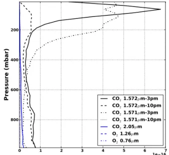
Figure 3.The variability in the differential optical depth weighting functions due to differences in NWP temperature and moisture as a function of vertical height. The values are the standard deviations of the difference between the average weighting function values and the ensemble members as a percentage of the mean weighting func-tion value.
1.571 and 1.572 µm wavelengths and 1.26 µm and 100 pm from center for the 2.051 and 0.76 µm wavelengths. The sub-traction of the offline OD in most of the cases has only a small effect on the total signal, with the exception of the 0.76 µm, due to the absence of aerosols in the LBLRTM cal-culations. In the real atmosphere, the presence of aerosols would add OD to the online and offline wavelengths in a sim-ilar way, but the DOD1τ would be comprised mostly of the trace gas to the total OD measurement. Figure 3 shows the ensemble standard deviation as a percentage of the ensemble mean WF for the1τmeasurement, which is the variability in
1τ
1P due to variations in temperature and moisture. The
vari-ability of the WFs due toT andQvariability is generally less than 10 % of the mean value, though there are differences be-tween the different instruments as to where the variability is largest.
Assuming that the differences in optical depths derived from NWP and observed environments have the same dis-tribution as the true errors, the sample error covarianceR1ξ
is computed by binning the differences into layers. The vari-ance for CO2and O2, as well as the in-layer covariance
be-tween CO2and O2, is computed. Between-layer error
corre-lations are assumed to be 0, which was necessary due to the heterogeneity in surface pressures (and hence the number of observations in each pressure layer) between sounding sites. The results using layer thicknesses of 25, 50 and 100 mb were examined, and there were no qualitative or quantita-tive differences. The results using 25 mb layers are depicted in Figs. 4 and 5. The 1.572 and 1.571 µm–3 pm variances are larger than the other instrument variances in the upper
tropo-0 1 2 3 4 5 6 1e 167
200
400
600
800
Pressure (mbar)
CO2 1.572µm-3pmCO2 1.572µm-10pm
CO2 1.571µm-3pm
CO2 1.571µm-10pm
CO2 2.05µm
O2 1.26µm
O2 0.76µm
Figure 4.The variance of the differences between differential op-tical depth WFs derived from observed and modeled atmospheric soundings as a function of pressure (in 25 mb layers). The enhanced variability in the 1.571 µm–3 pm and 1.572 µm–3 pm WFs is likely due to the strong gradients inT andQacross the tropopause, which can be located at different heights in NWP models versus rawinson-des, as is evident from Fig. 1.
sphere and stratosphere, which coincides with the elevatedT
errors in Fig. 1 that are likely due to the difficulty of predict-ing the strong gradients across the tropopause. Since these instruments’ WFs peak in this part of the atmosphere, they are the most susceptible to these errors propagating through the LBLRTM simulations. The rest of the instruments’ vari-ances fall between 0 and 1e-16, which corresponds to a stan-dard deviation of a small fraction (∼0.001 %) of the ensem-ble mean values depicted in Fig. 2 once the background mix-ing ratio contribution from CO2or O2has been removed.
4.2.3 Computation ofσ1ξ(h)
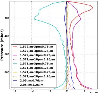
Applying Eq. (7) with the partial derivatives given by Eqs. (A7–A9) and the profiles in Figs. 4 and 5 and Eqs. (A7– A9) yieldsσ1ξ2 (h), for which the computed values are dis-played in Table 1. The magnitude of the 0.76 µm covariances shown in Fig. 5 carries through toσ1ξ
1τ CO2
1τO2
, and the re-sulting values are larger than the corresponding values for the 1.26 µm ratios. Only in the 1.572 µm–10 pm:1.26 µm case is the value ofσ1ξ
1τ CO2
1τO2
smaller as a percentage of the observation than that ofσ1ξ(1τCO2). This is significant be-cause smaller errors lead to larger information content, as-suming the sensitivities are comparable.
3 2 1 0 1 1e 19 200
400
600
800
Pressure (mbar)
1.572µm-3pm:0.76µm
1.572µm-3pm:1.26µm
1.572µm-10pm:0.76µm
1.572µm-10pm:1.26µm
1.571µm-3pm:0.76µm
1.571µm-3pm:1.26µm
1.571µm-10pm:0.76µm
1.571µm-10pm:1.26µm
2.05µm:0.76µm
2.05µm:1.26µm
Figure 5.The in-layer covariance of the differences between dif-ferential optical depths derived from observed and modeled atmo-spheric soundings, as a function of pressure (in 25 mb layers). The covariances between the CO2instruments and the 0.76 µm are uni-formly larger than those with the 1.26 µm instrument. Also, the 3 pm offset instruments have large covariances near the tropopause, which is consistent with Fig. 4.
Table 1. Temperature- and humidity-induced weighting function relative uncertainty for1τCO2 (first column) and 1τ1τCO2
O2 . The val-ues for σ1ξ(h)were computed using Eqs. (A7–A9) and the
pro-files in Figs. 4 and 5. The value for1τCO2 isσ 2
1ξ(1τCO2), while for 1τ1τCO2
O2 the relative uncertainty value is σ 2
1ξ
1τ
CO2
1τO2
1τO2
2. All computations assume constant profiles of 400 ppm of CO2and 21 % of O2. Note the larger magnitude of the 0.76 µm uncertainties, which arises from the larger covariances depicted in Fig. 5. Also note that only in the case of the 1.572 µm–10 pm CO2instrument paired with the 1.26 µm O2instrument is the ratio less sensitive to the environmental errors than the1τCO2 measurement alone.
O2line 0.76 µm 1.26 µm
CO2line 1τCO2
1τCO2 1τO2
1.572 µm–3 pm 1.719e-06 1.182e-05 1.767e-06 1.572 µm–10 pm 6.429e-07 1.962e-06 2.62e-07 1.571 µm–3 pm 2.15e-06 7.481e-06 4.121e-06 1.571 µm–10 pm 5.895e-08 8.193e-07 1.471e-07
2.051 µm 1.12e-07 1.563e-06 2.5e-07
the scope of this paper, and we assume that the state of the art radiative transfer models will be used in any operational retrievals.
4.3 The surface pressure uncertainty contribution
σp2∗(h)
In the context of surface pressure errors, with scalarshand
σ2(p∗), Eq. (7) implies
σp2∗(h)= ∂h
∂p∗ 2
σ2(p∗). (15)
Note that ∂p∂h∗ has been computed for1τCO2 and
1τCO2 1τO2 in
Eqs. (A5–A6).
The observed surface pressure values were extracted from 107 airport and/or permanent surface weather obser-vation station reports for the same contiguous United States (CONUS) and global regions described above along with their corresponding NWP model values. The NWP model values were corrected to the observed station height using a standard lapse rate relationship. The resulting 1σ value for the CONUS region was approximately 1.1 mbar and the 2σ
value was 2.1 mbar. The global region exhibited a 1σ value of 0.8 mbar and a 2σvalue of 1.7 mbar. Globally these obser-vations showed no significant biases and only slight seasonal variation in standard deviations. An in-depth discussion of the methods (including pressure correction for terrain height versus model represented terrain height) and analysis of these values is presented in Zaccheo et al. (2014).
The values ofσp∗(1τCO2)and1τO2σp∗ 1τ
CO2
1τO2
are dis-played in Table 2 forσNWP(p∗)values of 1mb and 2mb.
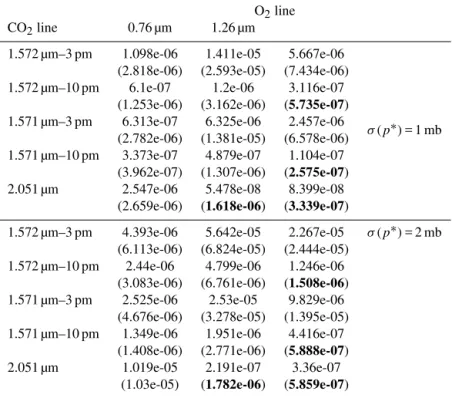
Sur-prisingly, in terms of relative uncertainty, the ratio observa-tions were not uniformly less sensitive to surface pressure errors than the1τCO2observations. The two weak CO2band
lidars with the 3 pm offset were actually less sensitive to sur-face pressure errors when no O2measurement was included.
This is due to the majority of their weight being concentrated near the tropopause and hence very little information coming from the surface. By contrast, the other two weak CO2band
instruments show a reduced sensitivity to errors in surface pressure from the inclusion of O2observations in the 1.26 µm
regime, and the strong CO2 band instrument benefits from
the inclusion of either O2observation in the 0.76 µm as well
as those at 1.26 µm. In parentheses is the sum of the surface pressure relative uncertainty and the WF relative uncertainty from Table 1. According to Eq. (14), the value in parentheses for 1τ1τCO2
O2 must be smaller than the value in parentheses for 1τCO2in order for there to be a useful O2measurement. The values that satisfy this criterion are printed in boldface.
5 Information-based Precision requirements for ASCENDS
Table 2.Surface pressure relative uncertainty for1τCO2and
1τCO2
1τO2 , with total environmental relative uncertainty in parentheses. The values
forσ1ξ(h)were computed using Eqs. (A5–A6) andσ (p∗)= 1 mb andσ (p∗)= 2 mb. The values in parentheses are the values from Table 1
added to the surface pressure relative uncertainties, and boldfaced values indicate instrument configurations for which an O2 lidar with enough precision could provide more information than the CO2only configuration with NWPp∗. Relative uncertainties areσp2∗(1τCO2) andσp2∗
1τ
CO2
1τO2
1τO2
2. All computations assume constant profiles of 400 ppm of CO2and 21 % of O2.
O2line
CO2line 0.76 µm 1.26 µm
1.572 µm–3 pm 1.098e-06 1.411e-05 5.667e-06
σ (p∗)= 1 mb (2.818e-06) (2.593e-05) (7.434e-06)
1.572 µm–10 pm 6.1e-07 1.2e-06 3.116e-07 (1.253e-06) (3.162e-06) (5.735e-07) 1.571 µm–3 pm 6.313e-07 6.325e-06 2.457e-06
(2.782e-06) (1.381e-05) (6.578e-06) 1.571 µm–10 pm 3.373e-07 4.879e-07 1.104e-07
(3.962e-07) (1.307e-06) (2.575e-07)
2.051 µm 2.547e-06 5.478e-08 8.399e-08
(2.659e-06) (1.618e-06) (3.339e-07)
1.572 µm–3 pm 4.393e-06 5.642e-05 2.267e-05 σ (p∗)= 2 mb (6.113e-06) (6.824e-05) (2.444e-05)
1.572 µm–10 pm 2.44e-06 4.799e-06 1.246e-06 (3.083e-06) (6.761e-06) (1.508e-06) 1.571 µm–3 pm 2.525e-06 2.53e-05 9.829e-06
(4.676e-06) (3.278e-05) (1.395e-05) 1.571 µm–10 pm 1.349e-06 1.951e-06 4.416e-07
(1.408e-06) (2.771e-06) (5.888e-07)
2.051 µm 1.019e-05 2.191e-07 3.36e-07
(1.03e-05) (1.782e-06) (5.859e-07)
expect that the O2 measurement error requirement should
match the pressure requirement, e.g., for a pressure error of 1 mb (about 0.1 % of a nominal 1000 mbp∗) we should have an O2measurement error of about 0.1 % or a SNR
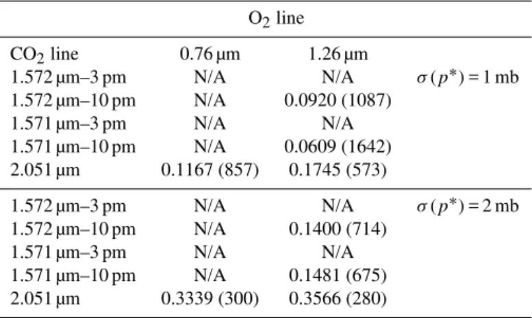
require-ment of 1000. Table 3 shows that the impact of including the environmentally induced errors as part of the calculation depends on the wavelengths of the CO2and O2instruments.
The 0.76 µm O2instrument column is N/A for each of the
pairings with the weak band CO2instruments, indicating that
no precision would be sufficient to provide a ratio measure-ment that improves on1τCO2 with NWPp
∗. This is largely due to the larger errors in the corresponding 1τ1τCO2
O2 observa-tion due to uncertainties in temperature and water vapor. The 0.76 µm O2measurement does have the potential to improve
upon the strong band CO2-only measurement, which is due
to the large sensitivity of the 2.051 µm instrument to surface pressure errors. This is evident in the fact that the doubling of surface pressure error from 1 to 2 mb relaxes the O2precision
requirement by nearly a factor of 3. Hence the environmental error contribution in the 0.76 µm line is overwhelmed by the surface pressure errors for the 2.051 µm line.
Examining the column for the 1.26 µm line we see that the smaller sensitivities to temperature and water vapor errors
in-crease the potential for improvement on two of the weak CO2
band instruments, namely those with the 10 pm offset. In this case, the surface pressure errors in these CO2only
observa-tions are large enough to offset the total errors in the ratio observations. For the 1.572 µm : 1.26 µm ratio, noted before because the ratio’s environmental errors are actually smaller than those of the CO2only observation, the minimum
preci-sion is smaller than that of the 1.571 µm ratio (i.e., SNR of 1087 vs. 1642 for 1 mb surface pressure errors). Doubling the surface pressure error again increases the precision but not by as large a factor as in the 0.76 µm case. This is not surprising, because the ratios using the 0.76 µm line have larger sensitiv-ities to surface pressure, as is evident in Table 2.
Perhaps most surprising is that our analysis concludes that neither O2measurement provides useful information to the
1.571 µm–3 pm or 1.572 µm–3 pm lines. This is due to the fact that these instruments are relatively insensitive to sur-face pressure errors due to their weighting function shapes. Thus, providing a high SNR O2measurement would have a
Table 3.Upper bounds on the O2measurement uncertaintyσobs(1τO2)computed from Eq. (13) expressed as percentages of a representative
1τO2 using 21 % atmospheric concentration and a typical vertical WF. The corresponding SNR lower bound is given in parentheses. For example, if the surface pressure error is 1 mb, the 0.76 µm precision would have to be smaller than 0.1167 % in order for the ratio with the strong band CO2measurement to provide a better constraint on model CO2than the CO2measurement alone using NWPp∗. The quantity N/A represents the scenarios in which Eq. (13) yielded a negative number, i.e., in which no O2instrument precision would yield a larger information content on modelqCO2than the corresponding1τCO2measurement using NWPp
∗.
O2line
CO2line 0.76 µm 1.26 µm
1.572 µm–3 pm N/A N/A σ (p∗)= 1 mb
1.572 µm–10 pm N/A 0.0920 (1087)
1.571 µm–3 pm N/A N/A
1.571 µm–10 pm N/A 0.0609 (1642)
2.051 µm 0.1167 (857) 0.1745 (573)
1.572 µm–3 pm N/A N/A σ (p∗)= 2 mb
1.572 µm–10 pm N/A 0.1400 (714)
1.571 µm–3 pm N/A N/A
1.571 µm–10 pm N/A 0.1481 (675)
2.051 µm 0.3339 (300) 0.3566 (280)
6 Conclusions
The preceding work defines an information-based measure-ment precision requiremeasure-ment for an O2instrument to provide
additional information on column CO2above and beyond a
CO2 measurement taken together with an NWP prediction
of surface pressure. The requirement includes the impacts of environmentally induced WF error correlations between the O2and CO2measurements as well as the expected
vari-ability of each due to surface pressure errors. Tests were per-formed using proxies for errors in the atmospheric state taken from NWP predictions and RAOBs for two different candi-date CO2and O2spectral lines. The major finding is that for
NWP surface pressure errors in the expected range of 1 to 2 mb Zaccheo et al. (2014), the contribution of the environ-mental uncertainty to the overall measurement requirement cannot be excluded in design considerations since for the 0.76 µm case these errors actually disqualified the instrument from being useful in conjunction with any weak CO2 band
lidar. The 1.26 µm instrument has more options for pairings but with smaller precision than would be expected from a pressure requirement alone for the weak CO2band. Both
struments do show the potential for providing additional in-formation on the 2.051 µm line, at a more relaxed precision requirement than the pressure would suggest. This is due to the reduced sensitivity of the ratio observations to surface pressure errors over the CO2observations alone.
The authors realize that we have only explored a small set of candidate wavelengths in the spectral bands of interest. We stress, however, that we are exploring exactly those lines be-ing targeted by current ASCENDS instrument design teams. It is beyond the scope of this paper to provide a complete characterization of all CO2and O2absorption figures. In the
event that other spectral lines are considered, this analysis will be repeated.
In the context of ever improving global NWP models, it is important to note that we expect global NWP surface pres-sure errors to trend toward the lower end of ourσ (p∗) spec-trum, which is 1mb or less. This being the case, justifying the expense for an active O2measurement can be expected
to become more difficult the longer that ASCENDS or other similar systems are delayed from launching. Tightening the precision of the lidar becomes more difficult and expensive the more accurate that NWP models become. It seems that the best option to avoid sensitivity to surface pressure errors is either a weak CO2band lidar with NWP atmospheric
vari-ables or a strong CO2band lidar paired with either of these
two O2lidars.
Acknowledgements. Crowell would like to acknowledge grant support from NASA Headquarters and the Langley Research Center (NASA). Rayner is in receipt of an Australian Professorial Fellowship (DP1096309). Zaccheo is funded in part by a grant from NASA Headquarters.
Appendix A: Discretized operators and their derivatives
Equations Eqs. (1–3) above are two examples of h. In the discrete case (i.e., in a numerical model), these observation operators are expressed using sums:
1τCO2= 1
mag nlayers
X
i=1 qCOi
2W
i
CO21p
i, (A1)
1τCO2 1τO2 =
Pnlayers
i=1 qCOi 2W
i
CO21p
i
Pnlayers
i=1 qOi2W
i
O21p
i . (A2)
The derivatives of the discrete observation operators Eqs. (A1–A2) with respect to the layer mixing ratios qCOi
2 are given by
∂1τCO2 ∂qCOi
2
=WCOi 21p
i, (A3)
∂
∂qCOi 2
1τCO2 1τO2
= W
i
CO21p
i
Pnlayers
j=1 q
j
O2W
j
O21p
j. (A4)
According to the fundamental theorem of calculus,
d dp∗
Rp∗
0 f (p)dp=f (p
∗), and so we define the derivatives of Eqs. (A1–A2) with respect top∗to satisfy this as closely as possible:
∂1τCO2 ∂p∗ =q
1 CO2W
1
CO2, (A5)
∂ ∂p∗
1τCO2 1τO2
=q
1 CO2W
1 CO2 1τO2
−q
1 O2W
1 O2 1τO2
1τCO2 1τO2
, (A6)
where the superscript 1 indicates the model surface layer. The derivatives of the observation operators with respect to the layer weighting functionsWi are
∂1τCO2
∂1ξCOi 2
=qCOi 21p
i, (A7)
∂
∂WCOi 2
1τCO2 1τO2
=
qCOi 21p
i
Pnlayers
j=1 q
j
O2W F
j
O21p
j, (A8)
∂
∂WOi 2
1τCO2 1τO2
= −
qO21p
iPnlayers
j=1 q
j
CO2W
j
CO21p
j
Pnlayers
j=1 qO2Wj1pj
References
Abshire, J., Ramanathan, A., Riris, H., Mao, J., Allan, G., Hassel-brack, W., Weaver, C., and Browell, E.: Airborne measurements of CO2Column Concentration and Range Using a Pulsed Direct-Detection IPDA Lidar, Remote Sens., 6, 443–469, 2014. Clough, S. et al.: Atmospheric radiative transfer modeling: a
sum-mary of the AER codes, Short Communication, J. Quant. Spec-trosc. Radiat. Transfer, 91, 233–244, 2005.
Devi, V., Benner, D., Brown, L., Miller, C., and Toth, R.: Line mixing and speed dependence in CO2 at 6227.9 cm−1: con-strained multispectrum analysis of intensities and line shapes in the 30013←00001 band, J. Mol. Spectrosc., 245, 52–80, 2007a. Devi, V., Benner, D., Brown, L., Miller, C., and Toth, R.: Line mix-ing and speed dependence in CO2at 6348 cm−1: positions, in-tensities, and air- and self-broadening derived with constrained multispectrum analysis, J. Mol. Spectrosc., 242, 90–117, 2007b. Houweling, S., Breon, F.-M., Aben, I., Rödenbeck, C., Gloor, M., Heimann, M., and Ciais, P.: Inverse modeling of CO2sources and sinks using satellite data: a synthetic inter-comparison of mea-surement techniques and their performance as a function of space and time, Atmos. Chem. Phys., 4, 523–538, doi:10.5194/acp-4-523-2004, 2004.
Hungershoefer, K., Breon, F.-M., Peylin, P., Chevallier, F., Rayner, P., Klonecki, A., Houweling, S., and Marshall, J.: Eval-uation of various observing systems for the global monitoring of CO2surface fluxes, Atmos. Chem. Phys., 10, 10503–10520, doi:10.5194/acp-10-10503-2010, 2010.
Miller, C. E., Crisp, D., DeCola, P. L., Olsen, S. C., Randerson, J. T., Michalak, A. M., Alkhaled, A., Rayner, P., Jacob, D. J., Suntharalingam, P., Jones, D. B. A., Denning, A. S., Nicholls, M. E., Doney, S. C., Pawson, S., Boesch, H., Connor, B. J., Fung, I. Y., O’Brien, D., Salawitch, R. J., Sander, S. P., Sen, B., Tans, P., Toon, G. C., Wennberg, P. O., Wofsy, S. C., Yung, Y. L., and Law, R. M.: Precision requirements for space-based data, J. Geophys. Res.-Atmos., 112, doi:10.1029/2006JD007659, 2007.
NASA: NASA ASCENDS Mission Science Definition and Planning Work-shop Report, Tech. rep., National Aeronau-tics and Space Agency, http://cce.nasa.gov/ascends/12-30-08% 20ASCENDS_Workshop_Report%20clean.pdf, 2008.
NCEP: The GFS Atmospheric Model, NOAA, Washington, D.C., 2003.
Rayner, P. J. and O’Brien, D. M.: The utility of remotely sensed CO2concentration data in surface source inversions, Geophys. Res. Lett., 28, 175–178, 2001.
Riris, H., Rodriguez, H., Allan, G., Hasselbrack, W., Mao, J., Stephen, M., and Abshire, J.: Pulsed airborne lidar measure-ments of atmospheric optical depth using the Oxygen A-band at 765 nm, Appl. Opt., 52, 6369–6382, 2013.
Rodgers, C.: Inverse methods for atmospheric sounding, in: Atmo-spheric, Ocean and Planetary Physics, World Scientific, World Scientific & Co., Singapore, 1–40, 2000.
Rogers, E., DiMego, G., Black, T., Ek, M., Ferrier, B., Gayno, G., Janjic, Z., Lin, Y., Pyle, M., Wong, V., Wu, B. S., and Carley, J.: The NCEP North American Mesoscale Model-ing System: Recent Changes and Future Plans, 2A.4, avail-able at: http://ams.confex.com/ams/pdfpapers/154114.pdf (last access: 7 July 2014), 2009.
Rothman, L. S., Gordon, I. E., Barbe, A., Benner, D. C., Bernath, P. F., Birke, M., Boudon, V., Brown, L. R., Campargue, A., Champion, J.-P., Chance, K., Coudert, L. H., Dana, V., Devi, V. M., Fally, S., Flaud, J.-M., Gamachel, R. R., Goldman, A., Jacquemart, D., Kleiner, I., Lacome, N., Lafferty, W. J., Mandin, J.-Y., Massie, S. T., Mikhailenko, S. N., Miller, C. E., Moazzen-Ahmadi, N., Naumenko, O. V., Nikitin, A. V., Orphal, J., Perevalov, V. I., Perrin, A., Predoi-Cross, A., Rinsland, C. P., Rotger, M., M. Sˇimeˇcková, Smith, M. A. H., Sung, K., Tashkun, S. A., Tennyson, J., Toth, R. A., Vandaele, A. C., Vander Auw-era, J.: The HITRAN 2008 molecular spectroscopic database, J. Quant. Spectrosc. Ra., 110, 533–572, 2009.
Sun, B., Reale, A., Seidel, D., and Hunt, D.: Comparing radiosonde and COSMIC atmospheric profile data to quantify differences among radiosonde types and the effects of imperfect collocation on comparison statistics, J. Geophys. Res.-Atmos., 115, D23104, doi:10.1029/2010jd014457, 2010.
Tarantola, A.: Inverse Problem Theory and Methods for Model Pa-rameter Estimation, SIAM, 2005.
Taylor, T., O’Dell, C., O’Brien, D., Kikuchi, N., Yokota, T., Naka-jima, T., Ishida, H., Crisp, D., and NakaNaka-jima, T.: Comparison of Cloud-Screening Methods Applied to GOSAT Near-Infrared Spectra, IEEE T. Geosci. Remote. Sens., 50, 295–308, 2012. US DOC/NOAA OFCM: Surface Weather Observations and
Re-ports, available at: http://www.ofcm.gov/fmh-1/fmh1.htm (last access: 07 July 2014), 2005.