Predicting classifier performance with limited training data: applications to computer-aided diagnosis in breast and prostate cancer.

Predicting Classifier Performance with

Limited Training Data: Applications to

Computer-Aided Diagnosis in Breast and

Prostate Cancer

Ajay Basavanhally, Satish Viswanath, Anant Madabhushi*

Department of Biomedical Engineering, Case Western Reserve University, Cleveland, OH, USA

*anantm@case.edu

Abstract

Clinical trials increasingly employ medical imaging data in conjunction with supervised clas-sifiers, where the latter require large amounts of training data to accurately model the sys-tem. Yet, a classifier selected at the start of the trial based on smaller and more accessible datasets may yield inaccurate and unstable classification performance. In this paper, we aim to address two common concerns in classifier selection for clinical trials: (1) predicting expected classifier performance for large datasets based on error rates calculated from smaller datasets and (2) the selection of appropriate classifiers based on expected perfor-mance for larger datasets. We present a framework for comparative evaluation of classifiers using only limited amounts of training data by using random repeated sampling (RRS) in conjunction with a cross-validation sampling strategy. Extrapolated error rates are subse-quently validated via comparison with leave-one-out cross-validation performed on a larger dataset. The ability to predict error rates as dataset size increases is demonstrated on both synthetic data as well as three different computational imaging tasks: detecting cancerous image regions in prostate histopathology, differentiating high and low grade cancer in breast histopathology, and detecting cancerous metavoxels in prostate magnetic resonance spec-troscopy. For each task, the relationships between 3 distinct classifiers (k-nearest neighbor, naive Bayes, Support Vector Machine) are explored. Further quantitative evaluation in terms of interquartile range (IQR) suggests that our approach consistently yields error rates with lower variability (mean IQRs of 0.0070, 0.0127, and 0.0140) than a traditional RRS ap-proach (mean IQRs of 0.0297, 0.0779, and 0.305) that does not employ cross-validation sampling for all three datasets.

Introduction

A growing amount of clinical research employs computerized classification of medical imaging data to develop quantitative and reproducible decision support tools [1–3]. A key issue during

a11111

OPEN ACCESS

Citation:Basavanhally A, Viswanath S, Madabhushi A (2015) Predicting Classifier Performance with Limited Training Data: Applications to Computer-Aided Diagnosis in Breast and Prostate Cancer. PLoS ONE 10(5): e0117900. doi:10.1371/journal. pone.0117900

Academic Editor:Benjamin Haibe-Kains, Princess Margaret Cancer Centre, CANADA

Received:August 6, 2014

Accepted:October 28, 2014

Published:May 18, 2015

Copyright:© 2015 Basavanhally et al. This is an open access article distributed under the terms of the Creative Commons Attribution License, which permits unrestricted use, distribution, and reproduction in any medium, provided the original author and source are credited.

Data Availability Statement:Data available from the Dryad Digital Repository. The data identifier is: doi:10. 5061/dryad.m5n98.

Funding:Research reported in this publication was supported by the National Cancer Institute of the National Institutes of Health under award numbers R01CA136535-01, R01CA140772-01,

R21CA167811-01, R21CA179327-01,

the development of image-based classifiers is the accrual of sufficient data to achieve a desired level of statistical power and, hence, confidence in the generalizability of the results. Computer-ized image analysis systems typically involve a supervised classifier that needs to be trained on a set of annotated examples, which are often provided by a medical expert who manually labels the samples according to their disease class (e.g. high or low grade cancer) [4]. Unfortunately, in many medical imaging applications, accumulating large cohorts is very difficult due to (1) the high cost of expert analysis and annotations and (2) because of overall data scarcity [3,5]. Hence, the ability to predict the amount of data required to achieve a desired classification ac-curacy for large-scale trials, based on experiments performed on smaller pilot studies is vital to the successful planning of clinical research.

Another issue in utilizing computerized image analysis for clinical research is the need to se-lect the best classifier at the onset of a large-scale clinical trial [6]. The selection of an optimal classifier for a specific dataset usually requires large amounts of annotated training data [7] since the error rate of a supervised classifier tends to decrease as training set size increases [8]. Yet, in clinical trials, this decision is often based on the assumption (which may not necessarily hold true [9]) that the relative performance of classifiers on a smaller dataset will remain the same as more data becomes available.

In this paper, we aim to overcome the major constraints on classifier selection in clinical tri-als that employ medical imaging data, namely (1) the selection of an optimal classifier using only a small subset of the full cohort and (2) the prediction of long-term performance in a clini-cal trial as data becomes available sequentially over time.

To this end, we aim to address crucial questions that arise early in the development in a clas-sification system, namely:

• Given a small pilot dataset, can we predict the error rates associated with a classifier assuming that a larger data cohort will become available in the future?

• Will the relative performance between multiple classifiers hold true as data cohorts grow larger?

Traditional power calculations aim to determine confidence in an error estimate using re-peated classification experiments [10], but do not address the question of how error rate changes as more data becomes available. Also, they may not be ideal for analyzing biomedical data because they assume an underlying Gaussian distribution and independence between vari-ables [11]. Repeated random sampling (RRS) approaches, which characterize trends in classifi-cation performance via repeated classificlassifi-cation using training sets of varying sizes, have thus become increasingly popular, especially for extrapolating error rates in genomic datasets [6,11,

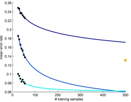
12]. Drawbacks of RRS include (1) no guarantee that all samples will be selected at least once for testing and (2) a large number of repetitions required to account for the variability associat-ed random sampling. In particular, traditional RRS may suffer in the presence of highly hetero-geneous datasets (e.g. biomedical imaging data [13]) due to the use of fixed training and testing pools. This is exemplified inFig 1by the variability in calculated (black boxes) and extrapolated (blue curves) error rates resulting from the use of different training and testing pools from the same dataset. More recently, methods such as repeated independent design and test (RIDT) [14] have aimed to improve RRS by simultaneously modeling the effects of different testing set sizes in addition to different training set sizes. This approach, however, requires allocation of larger testing sets than RRS, thereby reducing the number of samples available in the training set for extrapolation. It is important to note that the concept of predicting error rates for large datasets should not confused with semi-supervised learning techniques, e.g. active learning (AL) [15], that aim to maximize classifier performance while mitigating the costs of compiling

the DOD Lung Cancer Idea Development New Investigator Award (LC130463), the DOD Prostate Cancer Idea Development Award; the Ohio Third Frontier Technology development Grant, the CTSC Coulter Annual Pilot Grant, the Case Comprehensive Cancer Center Pilot Grant, VelaSano Grant from the Cleveland Clinic, the Wallace H. Coulter Foundation Program in the Department of Biomedical Engineering at Case Western Reserve University. The funders had no role in study design, data collection and analysis, decision to publish, or preparation of the manuscript. The content is solely the responsibility of the authors and does not necessarily represent the official views of the National Institutes of Health.

large annotated training datasets [5]. Since AL methods are designed to optimize classification accuracy during the acquisition of new data, they are not appropriate fora prioriprediction of classifier performance using only a small dataset.

Due to the heterogeneity present in biomedical imaging data, we extend the RRS-based ap-proach originally used to model gene microarray data [11] by incorporating aK-fold cross-vali-dation framework to ensure that all samples are used for both classifier training and testing (Fig 2). First, the dataset is split intoKdistinct, stratified pools where one pool is used for test-ing while the remaintest-ingK−1 are used for training. A bootstrap subsampling procedure is used to create multiple subsets of various sizes from the training pool. Each subset is used to train a classifier, which is then evaluated against the testing pool. The pools are rotatedKtimes to en-sure that all samples are evaluated once and error rates are averaged for each training set size. The resulting mean error rates are used to determine the three parameters of the power-law model (rate of learning, decay rate, and Bayes error) that characterize the behavior of error rate as a function of training set size.

Application of the RRS model to patient-level medical imaging data, where each patient or image is described by a single set of features, is relatively well-understood. Yet disease classifica-tion in radiological data (e.g. MRI) occurs at the pixel-level, in which each patient has pixels from both classes (e.g. diseased and non-diseased states) and each pixel is characterized by a set of features [16]. In this work, we present an extension to RRS that employs two-stage sam-pling in order to mitigate the samsam-pling bias occurring from high intra-patient correlation Fig 1. Traditional repeated random sampling (RRS) of prostate cancer histopathology leads to unstable estimation of error rates.Application of RRS to the classification of cancerous and non-cancerous prostate cancer histopathology (datasetD₁) suggests that heterogeneous medical imaging data can produce highly variable calculated (black boxes) and extrapolated (blue curves) mean error rates. Each set of error rates is derived from and independent RRS trial that employs different training and testing pools for classification. The yellow star represents the leave-one-out cross-validation error (i.e. the expected lower bound on error) produced by a larger validation cohort.

between pixels. The first stage requires all partitioning of the dataset to be performed at the pa-tient-level, ensuring that pixels from a single patient will not be included in both the training and testing sets. In the second stage, pixel-level classification is performed by training the clas-sifier using pixels from all images (and both classes) in the training set and evaluating against pixels from all images in the testing set. The resulting error rates are used to extrapolate classifi-er pclassifi-erformance as previously described for the traditional patient-level RRS.

This paper focuses on comparing the performance of three exemplar classifiers: (1) the non-parametrick-nearest neighbor (kNN) classifier [8], (2) the probabilistic naive Bayes (NB) clas-sifier that assumes an underlying Gaussian distribution [8], and (3) a non-probabilistic Support Vector Machine (SVM) classifier that aims to maximize class separation using a radial basis function (RBF) kernel. Each of these classifiers has previously been used for a variety of com-puterized image analysis tasks in the context of medical imaging [17,18]. All classifiers are evaluated on three distinct classification problems: (1) detection of cancerous image regions in prostate cancer (PCa) histopathology [5], (2) grading of cancerous nuclei in breast cancer (BCa) histopathology [19], and (3) detection of cancerous metavoxels on PCa magnetic reso-nance spectroscopy (MRS) [16].

The novel contributions of this work include (1) more stable learning curves due to the in-corporation of cross-validation into the RRS scheme, (2) a comparison of performance across multiple classifiers as dataset size increases, and (3) enabling a power analysis of classifiers op-erating on the pixel/voxel level (as opposed to patient/sample level), which cannot be currently done via standard sample power calculators.

The remainder of the paper is organized as follows. First, theMethodssection presents a de-scription of the methodology used in this work.Experimental Designincludes a description of Fig 2. A flowchart describing the methodology used in this paper.First, a dataset is partitioned into training and testing pools using aK-fold sampling strategy (red box). Each of theKtraining pools undergoes traditional repeated random sampling (RRS), in which error rates are calculated at different training set sizesnvia a subsampling procedure. A permutation test is used to identify statistically significant error rates, which are then used to extrapolate learning curves and predict error rates for larger datasets. The extension to pixel-level data employs the same sampling and error rate estimation strategies shown in this flowchart; however, the classifiers used for calculating the relevant error rates are trained and evaluated on pixel-level features from the training sets and testing pool, respectively.

the datasets and experimental parameters used for evaluation.Results and Discussionare sub-sequently presented for all experiments, followed byConcluding Remarks.

Methods

Notation

For all experiments, a datasetD_{is divided into independent training}ND_{and a testing}T D_{pools, where}N_\T_{=;. The class label of a samplex2}D_{is denoted byyt2{}ω_1,ω_{2}. A set of}

training set sizesN= {n1,n2,. . .,nN}, where 1n jNjandjjdenotes set cardinality.

Subsampling test to calculate error rates for multiple training set sizes

The estimation of classifier performance first requires the construction of multiple classifiers trained on repeated subsampling of the limited dataset. For each training set sizen2N, a total ofT1subsetsS(n)N, each containingnsamples, are created by randomly sampling the

training poolN_{. For eachn2Nandi2{1, 2,}. . .,T1}, the subsetSi(n)2Sis used to train a

cor-responding classifierHi(n). EachHi(n) is evaluated on the entire testing setTto produce an

error rateei(n). The mean error rate for eachn2Nis calculated as

eðnÞ ¼ 1

T1

XT1

i

eiðnÞ: ð1Þ

Permutation test to evaluate statistical significance of error rates

Permutation tests are a well-established, non-parametric approach for implicitly determining the null distribution of a test statistic and are primarily employed in situations involving small training sets that contain insufficient data to make assumptions about the underlying data dis-tribution [11,20]. In this work, the null hypothesis states that the performance of the actual classifier is similar to“intrinsic noise”of a randomly trained classifier. Here, a randomly trained classifier is modeled through repeated calculation of error rates from classifiers trained on data with randomly selected class labels.

To ensure the statistical significance of the mean error rateseðnÞcalculated inEq 1, the per-formance of training setSi(n) is compared against the performance of randomly labeled train-ing data. For eachSi(n)2S_{(n), a total ofT2subsets} S^_ðnÞ N_{, each containingnsamples, are}

created. For eachn2N,i2{1, 2,. . .,T1}, andj2{1, 2,. . .,T2}, the subset^Si;jðnÞ 2S^is

as-signed a randomized class labelyr2{ω_1,ω_{2} and used to train a corresponding classifier}

^

Hi;jðnÞ. EachH^i;jðnÞis evaluated on the entire testing setTto produce an error rate^ei;jðnÞ. For

eachn, a p-value

Pn¼

1 T1

1 T2

XT1

i¼1

XT2

j¼1

y_ðeðnÞ ^_ei;jðnÞÞ; ð2Þ

whereθ_{(z) = 1 ifz0 and 0 otherwise.Pnis calculated as the fraction of randomly-labeled}

classifiersH^i;jðnÞwith error ratesei;jðnÞexceeding the mean error rateeðnÞ;8n2N. The mean

error rateeðnÞis deemed to be valid for model-fitting only ifPn<0.05, i.e. there is a statistically

significant difference betweeneðnÞandf^_ei;jðnÞ;8i2 f1;2;. . .;T1g;8j2 f1;2;. . .;T2gg.

Hence, the set of valid training set sizesM= {n:n2N,Pn<0.05} includes only thosen2N

Cross-validation strategy for selection of training and testing pools

The selection of trainingN_{and testing}T_{pools from the limited dataset}D_{is governed by aK}

-fold cross-validation strategy. In this paper, the datasetD_{is partitioned intoK= 4 pools in}

which one pool is used for evaluation while the remainingK−1 pools are used for training to produce mean error ratesekðnÞ, wherek2{1, 2,. . .,K}. The pools are then rotated and the

sub-sampling and permutation tests are repeated until all pools have been evaluated exactly once. This process is repeated overRcross-validation trials, yielding mean error ratesek;rðnÞwherer

2{1, 2,. . .,R}. For all training set sizes that have passed the significance test, i.e.8n2M, learn-ing curves are generated from a comprehensive mean error rate

e_{ðnÞ ¼} 1

K 1 R

XK

k¼1

XR

r¼1

ek;rðnÞ; ð3Þ

calculated over all cross-validation foldsk2{1, 2,. . .,K} and iterationsr2{1, 2,. . .,R}.

Estimation of power law model parameters

The power-law model [11] describes the relationship between error rate and training set size

e_{ðnÞ ¼an} a_þ

b; ð4Þ

wheree_{ðnÞis the comprehensive mean error rate (Eq 3) for training set sizen,ais the learning}

rate, andαis the decay rate. The Bayes error ratebis defined as the lowest possible error given an infinite amount of training data [8]. The model parametersa,α, andbare calculated by solving the constrained non-linear minimization problem

min

a;a;b

XjMj

m¼1 ðan_mS a

þb e_ðnÞÞ2_{; ð5Þ}

wherea,α,b0.

Extension of error rate prediction to pixel- and voxel-level data

The methodology presented in this work can be extended to such pixel- or voxel-level data by first selecting training set sizesNat the patient-level. Definition of theKtraining and testing pools as well as creation of each subsampled training setSi(n)2S_{are also performed at the}

pa-tient-level. Training of the corresponding classifierHi(n), however, is performed at the pixel-level by aggregating pixels for all patients inSi(n). A similar aggregation is done for all patients in the testing poolT_{. By ensuring that all pixels from a given patient remain together, we are}

able to perform pixel-level calculations while avoiding the sampling bias that occurs when pix-els from a single patient span both training and testing sets.

Experimental Design

Our methodology is evaluated on a synthetic dataset and 3 actual classification tasks tradition-ally affected by limitations in the availability of imaging data (Table 1). All experiments have a number of parameters in common, includingT1= 50 subsampling trials,T2= 50 permutation

which allows us to maximize the number of training samples used for classification while yield-ing the expected lower bound of the error rate.

Ethics Statement

The three different datasets used in this study were retrospectively acquired from independent patient cohorts, where the data was initially acquired under written informed consent at each collecting institution. All 3 datasets comprised de-identified medical image data and provided to the authors through the IRB protocol # E09-481 titled“Computer-Aided Diagnosis of Can-cer”and approved by the Rutgers University Office of Research and Sponsored Programs. Fur-ther written informed consent was waived by the IRB board, as all data was being analyzed retrospectively, after de-identification.

Experiment 1: Identifying cancerous tissue in prostate cancer

histopathology

Automated systems for detecting PCa on biopsy specimens have the potential to act as (1) a tri-age mechanism to help pathologists spend less time analyzing samples without cancer and (2) an initial step for decision support systems that aim to quantify disease aggressiveness via auto-mated Gleason grading [5]. DatasetD_{1comprises anonymized hematoxylin and eosin (H & E)}

stained needle-core biopsies of prostate tissue digitized at 20x optical magnification on a whole-slide digital scanner. Regions corresponding to PCa were manually delineated by a pa-thologist and used as ground truth. Slides were divided into non-overlapping 30 × 30-pixel tis-sue regions and converted to a grayscale representation. A total of 927 features including first-order statistical, Haralick co-occurrence [21], and steerable Gabor filter features were extracted from each image [22] (Table 2). Due to the small number of training samples used in this study, the feature set was first reduced to two descriptors via the minimum redundancy maxi-mum relevance (mRMR) feature selection scheme [23], primarily to avoid the curse of di-mensionality [8]. A relatively small dataset of 100 image regions, with training set sizesN= {25, 30, 35, 40, 45, 50, 55}, was used to extrapolate error rates (Table 1). LOO cross-validation was subsequently performed on a larger dataset comprising 500 image regions.

Experiment 2: Distinguishing high and low tumor grade in breast cancer

histopathology

Nottingham, or modified Bloom-Richardson (mBR), grade is routinely used to characterize tumor differentiation in breast cancer (BCa) histopathology [24]; yet, it is known to suffer from high inter- and intra-pathologist variability [25]. Hence, researchers have aimed to devel-op quantitative and reproducible classification systems for differentiating mBR grade in BCa Table 1. List of the breast cancer and prostate cancer datasets used in this study.

Notation Description # train. samples # valid. samples

D₁ Prostate: Cancer detection on histopathology 100 500

D₂ Breast: Cancer grading on histopathology 46 116

D₃ Prostate: Cancer detection on MRS 16 34

ForD₁andD₂, each sample is treated independently during the selection of training and testing sets. ForD₃, training and testing sets are selected at the patient-level, while classification is performed at the metavoxel-level by using all metavoxels from both classes for a specified patient.

histopathology [19]. DatasetD_{2comprises 2000 × 2000 image regions taken from anonymized}

H & E stained histopathology specimens of breast tissue digitized at 20x optical magnification on a whole-slide digital scanner. Ground truth for each image was determined by an expert pa-thologist to be either low (mBR<6) or high (mBR>7) grade. First, boundaries of 30–40 rep-resentative epithelial nuclei were manually segmented in each image region (Fig 3). Using the segmented boundaries, a total of 2343 features were extracted from each nucleus to quantify Table 2. A summary of all features extracted from prostate cancer histopathology images in dataset

D₁.All textural features were extracted separately for red, green, and blue color channels.

Features Parameters

Texture: Gray-level (Average, Median, Standard Deviation, Range, Sobel, Kirsch, Gradient, Derivative)

window sizes: {3, 5, 7} Texture: Haralick co-occurrence (Joint Entropy, Energy,

Inertia, Inverse Difference Moment, Correlation, Measurements of Correlation, Sum Average, Sum Variance, Sum Entropy, Difference Average, Difference Variance, Difference Entropy, Shade, Prominence, Variance)

window sizes: {3, 5, 7}

Texture: steerable Gaborfilter responses (cosine and sine components combined)

window sizes: {3, 5, 7} frequency shift: {0, 1, . . ., 7} orientations:f0;p₈;2p₈;. . .;7p₈g

doi:10.1371/journal.pone.0117900.t002

Fig 3. Breast cancer (BCa) histopathology images from datasetD₂.Examples of (a), (b) low modified-Bloom-Richardson (mBR) grade and (c), (d) high mBR grade images are shown with boundary annotations (green outline) for exemplar nuclei. A variety of morphological and textural features are extracted from the nuclear regions, including (e)-(h) the Sum Variance Haralick textural response.

both nuclear morphology and nuclear texture (Table 3). A single feature vector was subse-quently defined for each image region by calculating the median feature values of all constitu-ent nuclei. Similar to Experimconstitu-ent 1, mRMR feature selection was used to isolate the two most important descriptors. Error rates were extrapolated from a small dataset comprising 45 images with training set sizesN= {20, 22, 24, 26, 28, 30, 32}, while LOO cross-validation was subse-quently performed on a larger dataset comprising 116 image regions (Table 1).

Experiment 3: Identifying cancerous metavoxels in prostate cancer

magnetic resonance spectroscopy

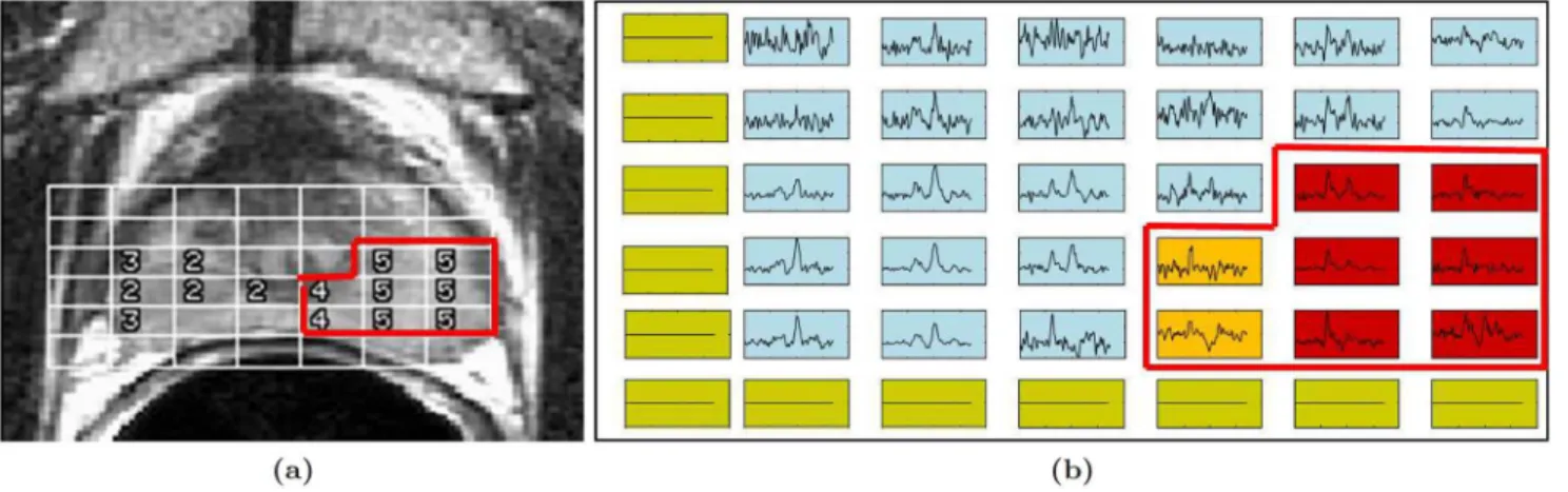
Magnetic resonance spectroscopy (MRS), a metabolic non-imaging modality that obtains the metabolic concentrations of specific molecular markers and biochemicals in the prostate, has previously been shown to supplement magnetic resonance imaging (MRI) in the detection of PCa [16,26]. These include choline, creatine, and citrate, and changes in their relative concen-trations (choline/citrate or [choline+creatine)/citrate], which have been shown to be linked to presence of PCa [27]. Radiologists typically assess presence of PCa on MRS by comparing ra-tios between choline, creatine, and citrate peaks to predefined normal ranges. DatasetD₃

com-prises 34 anonymized 1.5 Tesla T2-weighted MRI and MRS studies obtained prior to radical prostatectomy, where the ground truth was defined (as cancer and benign metavoxels) via visu-al inspection of MRI and MRS by an expert radiologist [16] (Fig 4). Six MRS features were de-fined for each metavoxel by calculating expression levels for each metabolite as well as ratios between each pair of metabolites. Similar to Experiment 1, mRMR feature selection was used to identify the two most important features in the dataset. Error rates were extrapolated from a dataset of 16 patients using training set sizesN= {2, 4, 6, 8, 10, 12}, followed by LOO cross-val-idation on a larger dataset of 34 patients (Table 1).

Comparison with traditional RRS via interquartile range (IQR)

This experiment compares the results of Experiment 1 with the traditional RRS approach, using both datasetD_{1and corresponding experimental parameters from Experiment 1.}

Table 3. A summary of all features extracted from breast cancer histopathology images in datasetD₂. All textural features were extracted separately for red, green, and blue color channels from the RGB color space and the hue, saturation, and intensity color channels from the HSV color space.

Features Parameters

Morphological: Basic (Area, Major Axis Length, Minor Axis Length, Eccentricity, Convex Area, Filled Area, Equivalent Diameter, Solidity, Extent, Perimeter, Area Overlap, Average Radial Ratio, Compactness, Convexity, Smoothness, Std. Dev. of Distance Ratio)

–

Morphological: Fourier Descriptors orientations:f0;p6; 2p

6;. . .; 5p

6g

Texture: Gray-level (Average, Median, Standard Deviation, Range, Sobel, Kirsch, Gradient, Derivative)

window sizes: {3, 5, 7}

Texture: Local binary patterns window size: 3 offsets: {0, 1,. . ., 7} directions: clockwise, counter-clockwise Texture: Laws (pairwise convolution of Level, Edge, Spot,

Wave, Ripplefilters) –

Texture: steerable Gaborfilter responses (cosine and sine components are separate features)

window sizes: {3, 5, 9} orientations:

f0;₁₂p;2p₁₂;. . .;6p₁₂g

However, since traditional RRS does not use cross-validation, a total ofT^1¼T1KR

sub-sampling procedures are used to ensure that same number of classification tasks are performed for both approaches. Evaluation is performed via (1) comparison of the learning curves be-tween the two methods and (2) the interquartile range (IQR), a measure of statistical variability defined as the difference between the 25th and 75th percentile error rates from the

subsampling procedure.

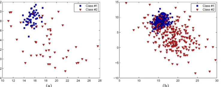
Synthetic experiment using pre-defined data distributions

The ability of our approach to produce accurate learning curves with low variance was evaluat-ed using a 2-class synthetic dataset, in which each class is definevaluat-ed by randomly selectevaluat-ed samples from a two-dimensional Gaussian distribution (Fig 5). Learning curves are created from a small dataset comprising 100 samples (Fig 5(a)) using training set sizesN= {25, 30, 35, 40, 45, 50, 55} in conjunction with a kNN classifier. Validation is subsequently performed on a larger dataset containing 500 samples (Fig 5(b)).

Results and Discussion

Experiment 1: Distinguishing cancerous and non-cancerous regions in

prostate histopathology

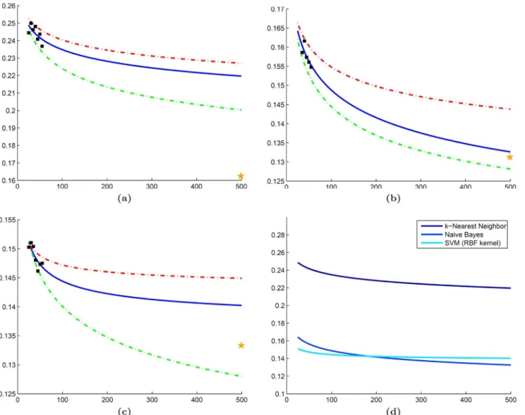
Error rates predicted by NB and SVM classifiers are similar to those from their LOO error rates of 0.1312 and 0.1333 (Fig6(b)and6(c)). In comparison to the learning curves, the slightly lower error rate produced by the validation set is to be expected since the LOO classification is known to produce an overly optimistic estimate of the true error rate [28]. The kNN classifier appears to overestimate error considerably compared to the LOO error of 0.1560, which is not surprising because kNN is a non-parametric classifier that is expected to be more unstable for heterogeneous datasets (Fig 6(a)). Comparison across classifiers suggests that both NB and SVM will outperform kNN as dataset size increases (Fig 6(d)). Although the differences be-tween the mean NB and SVM learning curves are minimal, the 25th and 75th percentile curves suggest that the prediction made by NB is more stable and has lower variance than the SVM prediction.

Fig 4. Magnetic resonance spectroscopy (MRS) data from datasetD₃.(a) A study from datasetD₃showing an MR image of the prostate with MRS metavoxel locations overlaid. (b) For ground truth, each MRS spectrum is labeled as either cancerous (red and orange boxes) or benign (blue boxes). Green boxes correspond to metavoxels outside the prostate for which MRS spectra were suppressed during acquisition.

Experiment 2: Distinguishing low and high grade cancer in breast

histopathology

Learning curves from kNN and NB classifiers yield predicted error rates similar to their LOO cross-validation errors (0.1552 for both classifiers) as shown in Fig7(a)and7(b). By contrast, while error rates predicted by the SVM classifier are reasonable (Fig 7(c)), they appear to un-derestimate the LOO error of 0.1724. One reason for this discrepancy may be the class imbal-ance present in the validation dataset (79 low grade and 37 high grade), since SVM classifiers have been demonstrated to perform poorly on datasets where the positive class (i.e. high grade) is underrepresented [29]. Similar toD_{1, a comparison between the learning curves reflects the}

superiority of both NB and SVM classifiers over the kNN classifier as dataset size increases (Fig 7(d)). However, the relationship between the NB and SVM classifiers is more complex. For small training sets, the NB classifier appears to outperform the SVM classifier; yet, the SVM classifier is predicted to yield lower error rates for larger datasets (n>60). This suggests that the classifier yielding the best results for the smaller dataset may not necessarily be the optimal classifier as the dataset increases in size.

Experiment 3: Distinguishing cancerous and non-Cancerous

metavoxels in prostate MRS

Similar to datasetD_{1, the LOO error for both the NB and SVM classifiers (0.2248 and 0.2468,}

respectively) fall within the range of the predicted error rates (Fig8(b)and8(c)). Once again, the kNN classifier overestimates the LOO error (0.2628), which is most likely due to the high level of variability in the mean error rates used for extrapolation (Fig 8(a)). While both NB and SVM classifiers outperform the kNN classifier, their learning curves show a clearer separation between the extrapolated error rates for all dataset sizes, suggesting that the optimal classifier selected from the smaller dataset will hold true as even as dataset size increases (Fig 8(d)). Fig 5. A synthetic dataset is used to validate our cross-validated repeated random sampling (RRS) method.In this dataset, each class is defined by samples drawn randomly from an independent two-dimensional Gaussian distribution. (a) A small set comprising 100 samples is used for creation of the learning curves and (b) a larger set comprising 500 samples is used for validation.

Comparison with traditional RRS

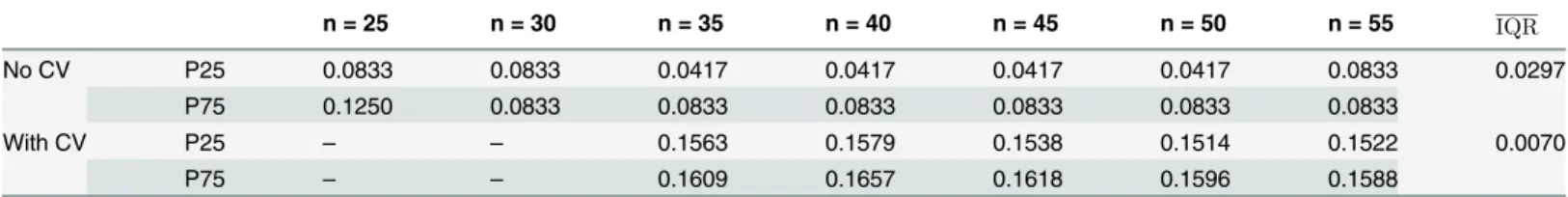
The quantitative results in Tables4–6suggest that employing a cross-validation sampling strat-egy yields more consistent error rates. InTable 4, traditional RRS yielded a mean IQR (IQRof 0.0297 across alln2N; whereas our approach demonstrated a lowerIQRof 0.0070. Further-more, a closer look at the learning curves for these error rates (Fig 9) suggests that traditional RRS is sometimes unable to accurately extrapolate learning curves. Similarly, Tables5and6

show lowerIQRvalues for our approach (0.0127 and 0.0140, respectively) than traditional RRS (0.0779 and 0.305, respectively) for datasetsD_2andD_{3. This phenomenon is most likely}

due to the high level of heterogeneity in medical imaging data and demonstrates the impor-tance of rotating the training and testing pools to avoid biased error rates that do not generalize to larger datasets.

Fig 6. Experimental results for datasetD₁.Learning curves (blue line) generated for datasetD₁using mean error rates (black squares) calculated from (a) kNN, (b) NB, and (c) SVM classifiers. Each classifier is accompanied by curves for the 25th (green dashed line) and 75th (red dashed line) percentile of the error as well as LOO error on the validation cohort (yellow star). (d) A direct classifier comparison is made in terms of the mean error rate predicted by each learning curve in (a)-(c).

Evaluation of synthetic dataset

The reduced variability of cross-validated RRS over traditional RRS is further validated by learning curves generated from the synthetic dataset (Fig 10). Error rates from our approach demonstrate low variability and the ability to create learning curves that can accurately predict the error rate of the validation set (Fig 10(b)). The cross-validated RRS approach yields a mean IQR (IQR= 0.0066) that is an order of magnitude less than traditional RRS (IQR= 0.074).

Concluding Remarks

The rapid development of biomedical imaging-based classification tasks has resulted in the need for predicting classifier performance for large data cohorts given only smaller pilot studies Fig 7. Experimental results for datasetD₂.Learning curves (blue line) generated for datasetD₂using mean error rates (black squares) calculated from (a) kNN, (b) NB, and (c) SVM classifiers. Each classifier is accompanied by curves for the 25th (green dashed line) and 75th (red dashed line) percentile of the error as well as LOO error on the validation cohort (yellow star). (d) A direct classifier comparison is made in terms of the mean error rate predicted by each learning curve in (a)-(c).

Fig 8. Experimental results for datasetD₃.Learning curves (blue line) generated for datasetD₃using mean error rates (black squares) calculated from (a) kNN, (b) NB, and (c) SVM classifiers. Each classifier is accompanied by curves for the 25th (green dashed line) and 75th (red dashed line) percentile of the error as well as LOO error on the validation cohort (yellow star). (d) A direct classifier comparison is made in terms of the mean error rate predicted by each learning curve in (a)-(c).

doi:10.1371/journal.pone.0117900.g008

Table 4. Mean interquartile range (IQR) demonstrates decreased variability of cross-validated random repeated sampling (RRS) over traditional RRS in datasetD1.

n = 25 n = 30 n = 35 n = 40 n = 45 n = 50 n = 55 IQR

No CV P25 0.0833 0.0833 0.0417 0.0417 0.0417 0.0417 0.0833 0.0297

P75 0.1250 0.0833 0.0833 0.0833 0.0833 0.0833 0.0833

With CV P25 – – 0.1563 0.1579 0.1538 0.1514 0.1522 0.0070

P75 – – 0.1609 0.1657 0.1618 0.1596 0.1588

A comparison between 25th (P25) and 75th (P75) percentile error rates for datasetD₁using traditional RRS (No CV) and our approach (With CV), with mean interquartile range (IQR) shown across alln. Missing values correspond to error rates that did not achieve significance in the permutation test.

Table 6. Mean interquartile range (IQR) demonstrates decreased variability of cross-validated random repeated sampling (RRS) over traditional RRS in datasetD3.

n = 2 n = 4 n = 6 n = 8 n = 10 n = 12 IQR

No CV P25 0.2242 0.2113 0.2113 0.2191 0.2294 0.2474 0.0305

P75 0.2809 0.2577 0.2500 0.2448 0.2448 0.2474

With CV P25 0.3176 0.3026 0.2950 0.2873 0.2874 0.2829 0.0140

P75 0.3345 0.3170 0.3065 0.3003 0.2993 0.2991

A comparison between 25th (P25) and 75th (P75) percentile error rates for datasetD₃using traditional RRS (No CV) and our approach (With CV), with mean interquartile range (IQR) shown across alln. Missing values correspond to error rates that did not achieve significance in the permutation test.

doi:10.1371/journal.pone.0117900.t006

Fig 9. Comparison between traditional random repeated sampling (RRS) and our cross-validated approach.Learning curves generated for dataset

D₁using (a) traditional RRS and (b) cross-validated RRS in conjunction with a Naive Bayes classifier. For both figures, mean error rates from the

subsampling procedure (black squares) are used to extrapolate learning curves (solid blue line). Corresponding learning curves for 25th (green dashed line) and 75th (red dashed line) percentile of the error are also shown. The error rate from leave-one-out cross-validation is illustrated by a yellow star.

doi:10.1371/journal.pone.0117900.g009

Table 5. Mean interquartile range (IQR) demonstrates decreased variability of cross-validated random repeated sampling (RRS) over traditional RRS in datasetD₂.

n = 20 n = 22 n = 24 n = 26 n = 28 n = 30 n = 32 IQR

No CV P25 0.1818 0.1818 0.1818 0.1818 0.1818 0.1818 0.1818 0.0779

P75 0.2727 0.2727 0.2727 0.2727 0.2727 0.2727 0.1818

With CV P25 0.2456 0.2489 0.2410 0.2347 0.2289 0.2311 0.2190 0.0127

P75 0.2456 0.2496 0.2494 0.2469 0.2506 0.2498 0.2463

A comparison between 25th (P25) and 75th (P75) percentile error rates for datasetD₂using traditional RRS (No CV) and our approach (With CV), with mean interquartile range (IQR) shown across alln. Missing values correspond to error rates that did not achieve significance in the permutation test.

with limited cohort sizes. This is important because, early in the development of a clinical trial, researchers need to: (1) predict long-term error rates when only small pilot studies may be available and (2) select the classifier that will yield the lowest error rates when large datasets are available in the future. Predicting classifier performance from small datasets is difficult because the resulting classifiers often produce unstable decisions and yield high error rates. In these sce-narios, traditional RRS approaches have previously been used to extrapolate classifier perfor-mance (e.g. for gene expression data). Due to the heterogeneity present in biomedical imaging data, we employ an extension of RRS in this work that uses cross-validation sampling to ensure that all samples are used for both training and testing the classifiers. In addition, we apply RRS to voxel-level studies where data from both classes is found within each patient study, a concept that has previously been unexplored in this regard. Evaluation was performed on three classifi-cation tasks, including cancer detection in prostate histopathology, cancer grading in breast histopathology, and cancer detection in prostate MRS.

We demonstrated the ability to calculate error rates with relatively low variance from three distinct classifiers (kNN, NB, and SVM). A direct comparison of the learning curves showed that the more robust NB and SVM classifiers yielded lower error rates than the kNN classifier for both small and large datasets. A limitation of this work is that all datasets comprise an equal number of samples from each class in order to reduce classifier bias from a machine learning standpoint. However, future work will focus on application to imbalanced datasets where class distribution is based on the overall population (e.g. clinical trials). In addition, we will incorporate additional improvements to the RRS method (e.g. subsampling of testing set as in RIDT) while maintaining a robust cross-validation sampling strategy. Additional direc-tions for future research include analyzing the effect of (a) noisy data on different classifiers [30] and (b) ensemble classification methods (e.g. Bagging) on classifier variability in small training sets.

Fig 10. Evaluation of our cross-validated repeated random sampling (RRS) on the synthetic dataset.Learning curves generated for the synthetic dataset using (a) traditional RRS and (b) cross-validated RRS in conjunction with a kNN classifier (k = 3). For both figures, mean error rates from the subsampling procedure (black squares) are used to extrapolate learning curves (solid blue line). Corresponding learning curves for 25th (green dashed line) and 75th (red dashed line) percentile of the error are also shown. The error rate from leave-one-out cross-validation is illustrated by a yellow star.

Supporting Information

S1 Appendix. Description of classifiers.Each experiment in this paper employs three

classifi-ers: k-nearest neighbor (kNN), Naive Bayes (NB), and Support Vector Machine (SVM). For ease of the reader we provide a metholodogical summary for each of these classifiers with ap-propriate descriptions and equations.

(PDF)

Acknowledgments

The authors would like to thank Dr. Scott Doyle for providing datasets used in this work.

Author Contributions

Conceived and designed the experiments: AB SV AM. Performed the experiments: AB. Ana-lyzed the data: AB SV AM. Contributed reagents/materials/analysis tools: AB SV AM. Wrote the paper: AB SV AM. Designed the software used in analysis: AB SV.

References

1. Evans AC, Frank JA, Antel J, Miller DH. The role of MRI in clinical trials of multiple sclerosis: compari-son of image processing techniques. Ann Neurol. 1997 Jan; 41(1):125–132. doi:10.1002/ana. 410410123PMID:9005878

2. Shin DS, Javornik NB, Berger JW. Computer-assisted, interactive fundus image processing for macular drusen quantitation. Ophthalmology. 1999 Jun; 106(6):1119–1125. doi:10.1016/S0161-6420(99) 90257-9PMID:10366080

3. Vasanji A, Hoover BA. Art & Science of Imaging Analytics. Applied Clinical Trials. 2013 March; 22 (3):38.

4. Madabhushi A, Agner S, Basavanhally A, Doyle S, Lee G. Computer-aided prognosis: Predicting pa-tient and disease outcome via quantitative fusion of multi-scale, multi-modal data. Computerized medi-cal imaging and graphics. 2011; 35(7):506–514. Available from:http://www.sciencedirect.com/science/ article/pii/S089561111100019X. doi:10.1016/j.compmedimag.2011.01.008PMID:21333490

5. Doyle S, Monaco J, Feldman M, Tomaszewski J, Madabhushi A. An active learning based classification strategy for the minority class problem: application to histopathology annotation. BMC bioinformatics. 2011; 12(1):424. doi:10.1186/1471-2105-12-424PMID:22034914

6. Berrar D, Bradbury I, Dubitzky W. Avoiding model selection bias in small-sample genomic datasets. Bioinformatics. 2006; 22(10):1245–1250. Available from:http://bioinformatics.oxfordjournals.org/ content/22/10/1245.short. doi:10.1093/bioinformatics/btl066PMID:16500931

7. Didaci L, Giacinto G, Roli F, Marcialis GL. A study on the performances of dynamic classifier selection based on local accuracy estimation. Pattern Recognition. 2005; 38. doi:10.1016/j.patcog.2005.02.010

8. Duda RO, Hart PE, Stork DG. Pattern Classification. Wiley; 2001.

9. Basavanhally A, Doyle S, Madabhushi A. Predicting classifier performance with a small training set: Ap-plications to computer-aided diagnosis and prognosis. In: Biomedical Imaging: From Nano to Macro, 2010 IEEE International Symposium on. IEEE; 2010. p. 229–232.

10. Adcock C. Sample size determination: a review. Journal of the Royal Statistical Society: Series D (The Statistician). 1997; 46(2):261–283. Available from: http://onlinelibrary.wiley.com/doi/10.1111/1467-9884.00082/abstract.

11. Mukherjee S, Tamayo P, Rogers S, Rifkin R, Engle A, Campbell C, et al. Estimating dataset size re-quirements for classifying DNA microarray data. J Comput Biol. 2003; 10(2):119–142. doi:10.1089/ 106652703321825928PMID:12804087

12. Dudoit S, Fridlyand J, Speed TP. Comparison of discrimination methods for the classification of tumors using gene expression data. Journal of the American statistical association. 2002; 97(457):77–87. doi: 10.1198/016214502753479248

14. Wickenberg-Bolin U, Göransson H, Fryknäs M, Gustafsson MG, Isaksson A. Improved variance esti-mation of classification performance via reduction of bias caused by small sample size. BMC bioinfor-matics. 2006; 7(1):127. doi:10.1186/1471-2105-7-127PMID:16533392

15. Freund Y, Seung HS, Shamir E, Tishby N. Selective sampling using the query by committee algorithm. Machine learning. 1997; 28(2–3):133–168. doi:10.1023/A:1007330508534

16. Tiwari P, Viswanath S, Kurhanewicz J, Sridhar A, Madabhushi A. Multimodal wavelet embedding repre-sentation for data combination (MaWERiC): integrating magnetic resonance imaging and spectroscopy for prostate cancer detection. NMR Biomed. t2012 Apr; 25(4):607–619. doi:10.1002/nbm.1777

17. Xu Y, van Beek EJ, Hwanjo Y, Guo J, McLennan G, Hoffman EA. Computer-aided classification of in-terstitial lung diseases via MDCT: 3D adaptive multiple feature method (3D AMFM). Academic radiolo-gy. 2006; 13(8):969–978. Available from:http://www.sciencedirect.com/science/article/pii/

S1076633206002716. doi:10.1016/j.acra.2006.04.017PMID:16843849

18. Sertel O, Kong J, Shimada H, Catalyurek U, Saltz JH, Gurcan MN. Computer-aided prognosis of neuro-blastoma on whole-slide images: Classification of stromal development. Pattern Recognition. 2009; 42 (6):1093–1103. Available from:http://www.sciencedirect.com/science/article/pii/S0031320308003439.

doi:10.1016/j.patcog.2008.08.027PMID:20161324

19. Basavanhally A, Ganesan S, Feldman M, Shih N, Mies C, Tomaszewski J, et al. Multi-Field-of-View Framework for Distinguishing Tumor Grade in ER+ Breast Cancer from Entire Histopathology Slides. IEEE Transactions on Biomedical Engineering. 2013; Available from:http://ieeexplore.ieee.org/xpls/ abs_all.jsp?arnumber=6450064. doi:10.1109/TBME.2013.2245129PMID:23392336

20. Good P. Permutation Tests: A Practical Guide to Resampling Methods for Testing Hypothesis. New York: Springer-Verlag; 1994.

21. Haralick RM, Shanmugam K, Dinstein IH. Textural features for image classification. Systems, Man and Cybernetics, IEEE Transactions on. 1973; SMC-3(6):610–621. Available from:http://ieeexplore.ieee. org/xpls/abs_all.jsp?arnumber=4309314. doi:10.1109/TSMC.1973.4309314

22. Doyle S, Feldman M, Tomaszewski J, Madabhushi A. A boosted bayesian multiresolution classifier for prostate cancer detection from digitized needle biopsies. Biomedical Engineering, IEEE Transactions on. 2012; 59(5):1205–1218. Available from:http://ieeexplore.ieee.org/xpls/abs_all.jsp?arnumber= 5491097. doi:10.1109/TBME.2010.2053540

23. Peng H, Long F, Ding C. Feature selection based on mutual information criteria of max-dependency, max-relevance, and min-redundancy. Pattern Analysis and Machine Intelligence, IEEE Transactions on. 2005; 27(8):1226–1238. Available from:http://ieeexplore.ieee.org/xpls/abs_all.jsp?arnumber= 1453511. doi:10.1109/TPAMI.2005.159

24. Elston C, Ellis I. Pathological prognostic factors in breast cancer. I. The value of histological grade in breast cancer: experience from a large study with long-term follow-up. Histopathology. 1991; 19 (5):403–410. doi:10.1111/j.1365-2559.1991.tb00229.xPMID:1757079

25. Meyer JS, Alvarez C, Milikowski C, Olson N, Russo I, Russo J, et al. Breast carcinoma malignancy grading by Bloom-Richardson system vs proliferation index: reproducibility of grade and advantages of proliferation index. Modern pathology. 2005; 18(8):1067–1078. Available from:http://www.nature.com/ modpathol/journal/vaop/ncurrent/full/3800388a.html. doi:10.1038/modpathol.3800388PMID:

15920556

26. Scheidler J, Hricak H, Vigneron DB, Yu KK, Sokolov DL, Huang LR, et al. Prostate cancer: localization with three-dimensional proton MR spectroscopic imaging-clinicopathologic study. Radiology. 1999 Nov; 213(2):473–480. doi:10.1148/radiology.213.2.r99nv23473PMID:10551229

27. Kurhanewicz J, Swanson MG, Nelson SJ, Vigneron DB. Combined magnetic resonance imaging and spectroscopic imaging approach to molecular imaging of prostate cancer. J Magn Reson Imaging. 2002 Oct; 16(4):451–463. doi:10.1002/jmri.10172PMID:12353259

28. Breiman L. Heuristics of instability and stabilization in model selection. The annals of statistics. 1996; 24(6):2350–2383. Available from:http://projecteuclid.org/euclid.aos/1032181158. doi:10.1214/aos/ 1032181158

29. Wu G, Chang EY. Class-boundary alignment for imbalanced dataset learning. In: ICML 2003 workshop on learning from imbalanced data sets II, Washington, DC; 2003. p. 49–56.