Qualitative Ferromagnetic Hysteresis Modeling

ISSN 1549-3636

© 2007 Science Publications

Corresponding Author: Mordjaoui Mourad, Electrical Engineering Department Skikda university BP: 26 Hadaiek 21000 Algeria

399

Qualitative Ferromagnetic Hysteresis Modeling

1

M. Mordjaoui, 3M.Chabane, 2B. Boudjema and 2R.Daira

1

Electrical Engineering Department, University of Skikda, Algeria

2

Fundamental Science Department, University of Skikda, Algeria

3

Electrical Engineering Department, University of Batna, Algeria

Abstract: In determining the electromagnetic properties of magnetic materials, hysteresis modeling is of high importance. Many models are available to investigate those characteristics but they tend to be complex and difficult to implement. A new qualitative hysteresis model for ferromagnetic core presented, based on the function approximation capabilities of adaptive neuro-fuzzy inference system (ANFIS). The proposed ANFIS model combined the neural network adaptive capabilities and the fuzzy logic qualitative approach can restored the hysteresis curve with a little RMS error. The model accuracy was good and can be easily adapted to the requirements of the application by extending or reducing the network training set and thus the required amount of measurement data.

Keywords: ANFIS modeling technique, magnetic hysteresis, Jiles-Atherton model, ferromagnetic core.

INTRODUCTION

Analysis of electrical machines requires a computationally efficient hysteresis model describing the nonlinear relation between the magnetic induction and the magnetic field strength in the ferromagnetic core of the machine. However, there exist many approaches to develop a mathematical model to describe the hysteretic relationship between the magnetization M and the magnetic field H. the first approach was the hysteresis model of Preisach invented in the 1935[1] and the second is the Jiles-Atherton (JA) model[2]. Artificial intelligence has also been applied to the modeling of magnetic hysteresis and parameters identification of these models such as neural network and genetic algorithm[3,4,5,6,7,8,9,10,11,12,13]. Like neural networks, fuzzy logic can be conveniently used to approximate any arbitrary functions[14,15,16]. Neural networks can learn from data, but knowledge learned can be difficult to understand. Models based on fuzzy logic are easy to understand, but they do not have learning algorithms; learning has to be adapted from other technologies. A Neuro-Fuzzy model can be defined as a model built using a combination of fuzzy logic and neural networks. Recently, there has been a remarkable advance in the development of Neuro-Fuzzy models, as it is described in[17,18,19]. One of the most popular and well documented Neuro-Fuzzy systems is ANFIS, which has a good software

support [20]. Jang[21,22,23] present the ANFIS architecture and application examples in modeling a nonlinear function, dynamic system identification and a chaotic time series prediction. Given its potential in building fuzzy models with good prediction capabilities, the ANFIS architecture was chosen for modeling magnetic hysteresis in this work. In the following sections information is given about adaptive neuro-Fuzzy modeling, the JA model for magnetic material testing system, the selection of ways to modeling the hysteresis phenomena with neuro-Fuzzy modeling, results and conclusions.

JILES-ATHERTON HYSTERESIS MODEL Formulation: The Jiles-Atherton model is a physically based model that includes the different mechanisms that take place at magnetization of a ferromagnetic material. The magnetization M is represented as the sum of the irreversible magnetization Mirr due to domain wall displacement and the reversible magnetization Mrev due to domain wall bending [2]. The rate of change of the irreversible part of the magnetization is given by.

) (

) (

0

M M k

M M dH

dM

an an irr

− −

− =

α δ µ

The anhysteretic magnetization Man in (1) follows the Langevin function [3], which is a nonlinear function of the effective field:

He=H+αM (2)

      −       = e e s an H a a H M

M coth (3)

The rate of change of the reversible component is proportional to the rate of the difference between the hysteretic component and the total magnetization [4]. Consequently, the differential of the reversible magnetization is:       − = dH dM dH dM c dH

dM rev an ₍₄₎

Combining the irreversible and reversible components of magnetization, the differential equation for the rate of change of the total magnetization is given by:

(

)

(

)

dH

dM c c M M k M M c dH dM _an an an 1 1 1 0 + + − − − + = α µ

δ (5)

Before using the J-A model, five parameters must be determined:

ƒ α: a mean field parameter defining the magnetic coupling between domains in the material, and is required to calculate the effective magnetic field, He (2) composed by the applied external field and the internal magnetization.

ƒ Ms: magnetic saturation ƒ a : langevin parameter

These two parameters defined a Langevin function needed in the equation describing anhysteretic curve.

ƒ k : parameter defining the pinning site density of domain walls. It is assumed to be the major contribution to hysteresis.

ƒ c : parameter defining the amount of reversible magnetization due to wall bowing and reversal rotation, included in the magnetization process.

ƒ δ is a directional parameter and takes +1 for increasing field (dH/dt>0) and -1 for decreasing field (dH/dt<0).

A. Parameter Identification B.1 Anhysteretic Susceptibility:

The anhysteretic susceptibility at the origin, can be used to define a relationship between Ms, a and α

0 0 = =













=

H M an an

dH

dM

χ

(6)

      + = α χ_an s M a 1 3 (7)

B.2 Initial susceptibility

The reversible magnetization component is expressed via the parameter c in the hysteresis equation (4) defined by:

α

χ

.

3

.

0 0 s M H ini

M

c

dH

dM

₌













=

= = (8) B.3 Coercivity

The hysteresis loss parameter k can be determined from the coercivity Hc and the differential susceptibility at the coercive point χan (Hc).

( )

( )

_                − − + − = dH dM c c H c H M k c c an 1 1

1 α _χ

(9)

B.3Remanence

The coupling parameter α can be determined independently if a is known by using the remanence magnetization Mr and the differential susceptibility at remanence.

( )

( )

M cdMdH c a k M M M r r an r − + − + = χ 1 1 (10)

ADAPTIVE NEURO-FUZZY INFERENCE SYSTEM (ANFIS) An adaptive Neuro-Fuzzy inference system is a cross between an artificial neural network and a fuzzy inference system. An artificial neural network is designed to mimic the characteristics of the human brain and consists of a collection of artificial neurons. An adaptive network is a multi-layer feed-forward network in which each node (neuron) performs a particular function on incoming signals. The form of the node functions may vary from node to node. In an adaptive network, there are two types of nodes: adaptive and fixed. The function and the grouping of the neurons are dependent on the overall function of the network. . Based on the ability of an ANFIS to learn from training data, it is possible to create an ANFIS structure from an extremely limited mathematical representation of the system.

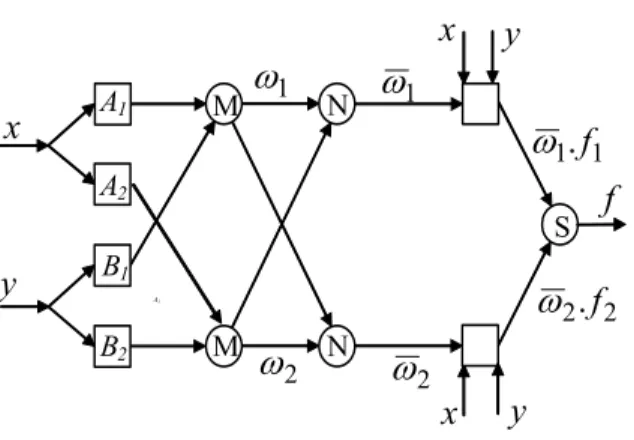
are two input linguistic variables (x, y) and each variable has two fuzzy sets (A1, A2) and ( B1,B2) as is indicated in fig.1, in which a circle indicates a fixed node, whereas a square indicates an adaptive node. Then a Takagi-Sugeno-type fuzzy if-then rule could be set up as:

Rule i: If (x is Ai) and (y is Bi) then (fi = pix + qiy + ri)

x

A1

1

ω

_ω

₁

2

ω

2

ω

2 2

.

f

ω

1 1

.

f

ω

x

y

y

y

x

A1

A2

B1

B2

M

M

N

N

f

S

Fig. 1: ANFIS architecture

fi are the outputs within the fuzzy region specified by the fuzzy rule. pi, qi and ri are the design parameters that are determined during the training process.

Some layers of ANFIS have the same number of nodes, and nodes in the same layer have similar functions

.

Output of nodes in layer-l is denoted as

O

_i1, where l is the layer umber and i is neuron number of the next layer. The function of each layer is described as follows:

Layer 1: In this layer, all the nodes are adaptive nodes. The outputs of layer 1 are the fuzzy membership grade of the inputs, which are given by:

2

,

1

)

(

1

=

=

i

x

O

i

A

i

µ

(11)

4

,

3

)

(

2

1

=

=

−

y

i

O

i

B

i

µ

(12)

Where

(

),

(

)

2

y

x

i

i B

A

µ

₋

µ

can adopt any fuzzy

membership function. For example, if the bell shaped membership function is employed,

(

x

)

i

A

µ

is given by:

i

i i A

b

a c x x

i

    

  

      − + =

2

1 1 )

(

µ (13)

where ai, bi and ci are the parameters of the membership function, governing the bell shaped functions accordingly.

• Layer 2:Each node computes the firing strengths of the associated rules. The output of nodes in this layer can be presented as:

2 , 1 )

( ) (

2 = = _{x y i}=

O

i

i B

A i

i

ω

µ

µ

(14)

Layer 3: In this third layer, the nodes are also fixed nodes. They play a normalization role to the firing strengths from the previous layer. The outputs of this layer can be represented as:

2 , 1 2

1

3 ₌

+ =

= i

O i

i

i

_ω

_ω

ω

ω

(15)

which are the so-called normalized firing levels. • Layer 4: The output of each adaptive node in this layer is simply the product of the normalized firing level and a first order polynomial (for a first order Sugeno model). Thus, the outputs of this layer are given by:

(

)

1,2

4 _{= = + + =}

i r y q x p f

O_i

ω

_{i i}

ω

_{i i i i} (16)

• Layer 5: Finally, layer five, consisting of circle node labeled with S. is the summation of all incoming signals. Hence , the overall output of the model is given by:

2 1

2

1 2

1 5

ω

ω

ω

ω

+

=

=

∑

∑

=

=

i i i

i i i i

f

f

O

(17)

From the architecture of ANFIS, we can observe that there are two adaptive layers the first and the fourth. In the first layer, there are three modifiable parameters {ai, bi, ci}, which are related to the input membership functions. These parameters are the so-called premise parameters. In the fourth layer, there are also three modifiable parameters {pi,qi,ri}, pertaining to the first order polynomial. These parameters are so-called consequent parameters [21-22].

2 2 1 2 1 2 1 1

f

f

f

ω

ω

ω

ω

ω

ω

+

+

+

=

(18)

Substituting Eq. (15)into Eq. (18)yields:

2 2 1

1

f

f

f

=

ω

+

ω

(19)

Substituting the fuzzy if-then rules into equation (19), it becomes:

(

1 1 1

)

2

(

2 2 2

)

1 p x q y r p x q y r

f =ω + + +ω + + (20)

After rearrangement, the output can be expressed as:

( )

( )

( )

( )

2 2

(

2

)

2

( )

2 2 1 1 1 1 1 1 . . . . . . r q y p x r q y p x f ω ω ω ω ω ω + + + + + = (21)

This is a linear combination of the modifiable parameters. For this observation, we can divide the parameter set S into two sets:

S=S1

⊕

S2

S=set of total parameters,

S1=set of premise (nonlinear) parameters, S2=set of consequent (linear) parameters

⊕

: Direct sum

For the forward path (see Fig 1), we can apply least square method to identify the consequent parameters. Now for a given set of values of S1, we can plug training data and obtain a matrix equation:

y

A

Θ

=

(22)

where Θ contains the unknown parameters in S2. This is a linear square problem, and the solution for Θ, which is minimizes

A

Θ

=

y

, is the least square estimator:

( )

A

T

A

−1

A

T

y

∗

₌

Θ

(23)

we can use also recursive least square estimator in case of on-line training. For the backward path (see Fig. 1), the error signals propagate backward. The premise parameters are updated by descent method, through minimising the overall quadratic cost function

( )

_∑

[

]

= Θ − = Θ N N k y k y J 1 2 ) , ( ) ( 2 1 (24)

in a recursive manner with respect Θ(S2). The update of the parameters in the ith node in layer Lth layer can be written as: ) ( ˆ ) ( ) 1 ( ˆ ) ( ˆ k k E k k L i L i i Θ ∂ ∂ + − Θ =

Θ η + (25)

where η is the learning rate and the gradient vector

L i i L i L L i

z

E

Θ

∂

∂

=

Θ

∂

∂

+

ˆ

ˆ

ˆ

, ,

ε

(26)

i L

z

ˆ

_,

∂

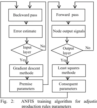
being the node’s output and

ε

_L,i is the backpropagated error signal. Fig.2 presents the ANFIS training algorithm for adjusting production rules parameters.

Backward pass Forward pass

Error estimate Node output signals

Gradient descent methode Least squares methode Premise parameters Consequent parameters

Yes Yes

No _No

Input

layer Output _layer

Fig. 2: ANFIS training algorithm for adjusting production rules parameters

APPROXIMATING MAGNETIC HYSTERESIS

Simulation: The differential equation (5), which in its original form has derivatives with respect to H , was reformulated into a differential equation in time by multiplying the left and the right sides by

dH

dt

, thus resulting in:

(

)

(

)

dt

dM c c M M k M M dt dH c dt dM _an an an + + − − − + = 1 . . 1 1 0 α µ

δ (27)

This reformulation allows for the determination of magnetization by use of Runge Kutta method in Matlab environment.

To calculate the magnetic flux density B from M and H, the following constitutive law of the magnetic material property is used.

(

H

M

)

H

H

B

=

µ

.

=

µ

₀

µ

_r

=

µ

₀

+

(28) Where µ0=4.π.10-7 (H/m) is the permeability of free space and µr is the relative permeability.

Proposed model: In this section, the learning ability of ANFIS is verified by approximating a hysteresis of magnetic material. The data set used as input/output pairs for Anfis was generated by Jiles Atherton model for ferrite core described in [24] with sinusoidal magnetic field as an input H(t) and magnetic field B(t) as output Fig. (3.a & b).

(a)

(b)

Fig.3: a- Normalized magnetic field and magnetic versus time b- Normalized magnetic induction versus time

Our purpose is to predict the magnetic hysteresis cycles using 12 candidate inputs to ANFIS : B(t-i) for i=1 :5, and H(t-j) for j=1 :7. Converted from the original data sets containing 353 [H(t) B(t)] pairs.

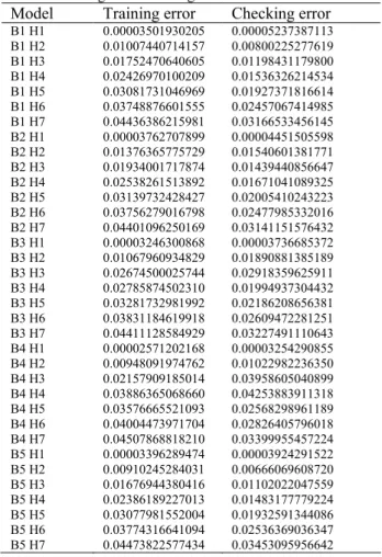
In the first time, we suppose that there are two inputs for ANFIS and wehave to construct 35 ANFIS models (5x7) with various input combinations, and then select the one with the smallest training error for further parameter-level fine tuning. In table.I we can see that the ANFIS with B4 and H1 (in red) as inputs has the smallest training error, so it is reasonable to choose this ANFIS for further parameter tuning. Note that each ANFIS has four rules, and the training took only one epoch each to identify linear parameters. Let us note that the computing time for selecting the good model is 3.6250s.

Table 1: Training And Checking Error For All Models Model Training error Checking error

B1 H1 0.00003501930205 0.00005237387113 B1 H2 0.01007440714157 0.00800225277619 B1 H3 0.01752470640605 0.01198431179800 B1 H4 0.02426970100209 0.01536326214534 B1 H5 0.03081731046969 0.01927371816614 B1 H6 0.03748876601555 0.02457067414985 B1 H7 0.04436386215981 0.03166533456145 B2 H1 0.00003762707899 0.00004451505598 B2 H2 0.01376365775729 0.01540601381771 B2 H3 0.01934001717874 0.01439440856647 B2 H4 0.02538261513892 0.01671041089325 B2 H5 0.03139732428427 0.02005410243223 B2 H6 0.03756279016798 0.02477985332016 B2 H7 0.04401096250169 0.03141151576432 B3 H1 0.00003246300868 0.00003736685372 B3 H2 0.01067960934829 0.01890881385189 B3 H3 0.02674500025744 0.02918359625911 B3 H4 0.02785874502310 0.01994937304432 B3 H5 0.03281732981992 0.02186208656381 B3 H6 0.03831184619918 0.02609472281251 B3 H7 0.04411128584929 0.03227491110643 B4 H1 0.00002571202168 0.00003254290855 B4 H2 0.00948091974762 0.01022982236350 B4 H3 0.02157909185014 0.03958605040899 B4 H4 0.03886365068660 0.04253883911318 B4 H5 0.03576665521093 0.02568298961189 B4 H6 0.04004473971704 0.02826405796018 B4 H7 0.04507868818210 0.03399955457224 B5 H1 0.00003396289474 0.00003924291522 B5 H2 0.00910245284031 0.00666069608720 B5 H3 0.01676944380416 0.01102022047559 B5 H4 0.02386189227013 0.01483177779224 B5 H5 0.03077981552004 0.01932591344086 B5 H6 0.03774316641094 0.02536369036347 B5 H7 0.04473822577434 0.03453095956642

After selection of the good and adapted model, we made train the network 100 epochs, for this purpose we have used 173 pairs as training data and 173 pairs for checking, shown in fig.3.

Fig.4 : Data distribution

set after every iteration, by calculating the root-mean-square errors (RMSE):

(

)

K y y

RMSE

K

k

k k

∑

=

− = 1

(28) Where k is the pattern number, k=1,…K. The RMSE was also evaluated on training data set in every iteration. The optimal number of iteration was obtained when checking RMSE has reached its minimum value 0.0069 after 11 epochs. See fig.5.

Fig.5: Error curves

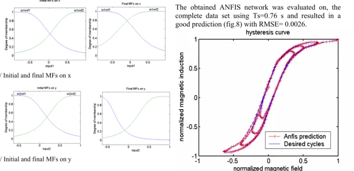
Fig.6 depicts the initial and final membership functions for each input variable. The anfis used here contains a total of 24. fitting parameters, of which 12 are presmise (nonlinear) parameters and 12 are consequent (linear) parameters. Table.II summarize all characteristics of the network used.

a/ Initial and final MFs on x

b/ Initial and final MFs on y

Fig. 6: Initial and final generalized bell-shaped membership function of input 1 and 2 for the Best model.

Table 2: ANFIS Caracteristics

Number of nodes 21

Number of linear parameters 12 Number of nonlinear parameters 12 Total number of parameters 24 Number of training data pairs 173 Number of checking data pairs 173

Number of fuzzy rules 04

The ANFIS shown in Fig.1 was implemented by using MATLAB software package ( MATLAB version 6.5 with fuzzy logic toolbox), it uses 346 training data in 100 training periods and the step size for parameter adaptation had an initial value of 0.1. The steps of parameter adaptation of the ANFIS are shown in Fig.7.

Fig. 7: Adaptation of parameter steps of ANFIS

The obtained ANFIS network was evaluated on, the complete data set using Ts=0.76 s and resulted in a good prediction (fig.8) with RMSE= 0.0026.

CONCLUSION

We have successfully developed, implemented and tested a neurofuzzy system for predicting the magnetic hysteresis of ferromagnetic core. It is clear that the system output closely approximates the required hysteresis output by Jiles-Atherton model.

The proposed model is an alternative and less complicated approach in determining the magnetic properties of ferromagnetic materials with good accuracy. The collection of well-distributed, sufficient, and accurately measured input data is the basic requirement to obtain an accurate model. The adequate functioning of ANFIS depends on the sizes of the training set and test set. Simulation result revealed that neuro-fuzzy model was capable of closely reproducing the optimal performance. In the future studies, we will incorporate this model on the finite element procedure for modeling electromagnetic devices.

REFERENCES

1. F. Preisach, 1938. On magnetic after-effect. journal of physics, vol. 94, no. 5–6, p. 277.

2. D. C. Jiles and D. L. Atherton, 1986. Theory of ferromagnetic hysteresis. J.Magn. Magn. Mater., vol. 61, pp. 48–60.

3. K. P. R. Wilson, J. N. Ross, and A. D. Brown, 2001. Optimizing the Jiles–Atherton model of hysteresis by a genetic algorithm. IEEE Trans. Magn., vol. 37, pp. 989–993.

4. A. Salvini and F. Riganti Fulginei, 2002. Genetic algorithms and neural networks loops. IEEE Trans. Magn., vol. 38, pp. 873–876.

5. A. Salvini and C. Coltelli, 2001. Prediction of dynamic hysteresis under highly distorted exciting fields by neural networks and actual frequency transplantation. IEEE Trans. Magn., vol. 37, pp. 3315–3319.

6. P. Del Vecchio and A. Salvini, 2001. Neural networks and Fourier descriptor macromodeling dynamic hysteresis. IEEE Trans. Magn., vol. 36, pp. 1246–1249.

7. Q. Xu, A. Refsum, 1997. Neural network for represention of hysteresis loops. IEE proc-Sci Meas technol, Vol 144, No. 6, pp 263-266.

8. H. H. Saliah and D. D. Lowther, 1997. A Neural Network Nodel of Magnetic Hysteresis for computational magnetics. IEEE Trans. Magn., vol 33, N° 05, pp 4146-4148.

9. Dimitre Makaveev, Luc Dupre´ , Marc De Wulf, and Jan Melkebeek, 2001. modeling of quasistatic hysteresis with feed-forwad neural networks. journal of applied physics, volume 99, N° 11, pp 6737-6739.

10. Dimitre Makaveev, Luc Dupre, Marc De Wulf, and Jan Melkebeek, 2003. Combined Preisach– Mayergoyz-neural-network vector hysteresis model for electrical steel sheets. journal of applied physics, volume 93, N° 10, pp 6738-6740.

11. M. Saghafifar, A. Nafalski, 2002. Magnetic hysteresis modeling using dynamic neural networks. Japan Society of Applied Electromagnetics and Mechanics (JSAEM) Studies in Applied Electromagnetics and Mechanics, vol. 14, JSAEM, Kanazawa, Japan, pp.293-299.

12. M. Kuczmann, A. Iványi, 2002. A New Neural-Network-Based Scalar Hysteresis Model. IEEE Trans. on Magn., vol.38, no.2, pp. 857-860.

13. M. Kuczmann, A. Iványi, 2002. Neural Network Model of Magnetic Hysteresis. Compel, vol.21, no.3, pp. 364-376.

14. Zadeh LA. 1965 Fuzzy sets. Information and Control, 8: 338–353.

15. Buckley JJ, Hayashi Y, 1994. Hybrid fuzzy neural nets are universal approximators. Proc IEEE Int Conf on Fuzzy Systems, Orlando, FL, 238–243. 16. Kosko B, 1992. Fuzzy systems as universal

approximators. Proc IEEE Int Conf on Fuzzy Systems, San Diego, CA, 1153–1162.

17. J. Yen and R. Langari, 1999. Fuzzy Logic, Intelligence, Control and Information. Prentice Hall.

18. J. S. Jang, C.-T. Sun and E. Mizutani, 1997. Neuro-Fuzzy and Soft Computing. Prentice Hall. 19. A. Abraham. 2001. Neuro-Fuzzy Systems:

State-of-the-art Modeling Techniques. In J. Mira and A. Prieto (Eds), Connectionist Models of Neurons, Learning Processes, and Artificial Intelligence, Springer- Verlag, pp. 269-276.

20. The MathWorks, Inc., 1998. Fuzzy Logic Toolbox. 21. J. S. Jang, 1993. ANFIS: Adaptive-network-based fuzzy Inference Systems. IEEE Transactions on Systems, Man and Cybernetics. Part B: Cybernetics, vol. 23, pp. 665-685.

22. Jang J-SR. 1992. Self-learning fuzzy controllers based on temporal backpropagation. IEEE Trans Neural Netw 3(5):714–23.

23. J.S.Roger Jang, C.T. Sun, 1995. Neuro-Fuzzy Modeling And Control, Proceeding of the IEEE, vol.83, No.3.