The Search for Significance: A Few
Peculiarities in the Distribution of
P
Values
in Experimental Psychology Literature
MichałKrawczyk*
University of Warsaw, Dluga 44/50, 00–241, Warsaw, Poland
*mkrawczyk@wne.uw.edu.pl
Abstract
In this project I investigate the use and possible misuse ofpvalues in papers published in five (high-ranked) journals in experimental psychology. I use a data set of over 135’000p
values from more than five thousand papers. I inspect (1) the way in which thepvalues are reported and (2) their distribution. The main findings are following: first, it appears that some authors choose the mode of reporting their results in an arbitrary way. Moreover, they often end up doing it in such a way that makes their findings seem more statistically significant than they really are (which is well known to improve the chances for publication). Specifical-ly, they frequently reportpvalues“just above”significance thresholds directly, whereas other values are reported by means of inequalities (e.g.“p<.1”), they round thepvalues down more eagerly than up and appear to choose between the significance thresholds and between one- and two-sided tests only after seeing the data. Further, about 9.2% of re-portedpvalues are inconsistent with their underlying statistics (e.g.Fort) and it appears that there are“too many” “just significant”values. One interpretation of this is that research-ers tend to choose the model or include/discard observations to bring thepvalue to the right side of the threshold.
Introduction
Statistics is the corner stone of nearly all empirical science. It provides the essential tools to dis-tinguish between the systematic and the incidental. However, the power of statistics brings with it the possibility of abuse. Most authors are well aware of the fact that the statistics in their papers (notably: the statistical significance of the effects they are reporting) may substantially affect their publishability (“publication bias”) and also their impact. If so, we can expect them to employ what we can call strategic reporting: to include those results and in such a way that favors their theories [1,2].
For the purpose of this study a large data set of statistics (pvalues and otherwise) reported in about 5’000 papers has been collected and investigated. I find evidence suggesting that vari-ous types of decisions (e.g., whether or not to round given number and whether to use a
one-OPEN ACCESS
Citation:Krawczyk M (2015) The Search for
Significance: A Few Peculiarities in the Distribution of PValues in Experimental Psychology Literature. PLoS ONE 10(6): e0127872. doi:10.1371/journal. pone.0127872
Academic Editor:Daniele Fanelli, Stanford
University, UNITED STATES
Received:October 16, 2013
Accepted:April 20, 2015
Published:June 10, 2015
Copyright:© 2015 MichałKrawczyk. This is an open
access article distributed under the terms of the Creative Commons Attribution License, which permits unrestricted use, distribution, and reproduction in any medium, provided the original author and source are credited.
Funding:The author acknowledges financial support
from the European Commission under the ERG ACADIS project. The funders had no role in study design, data collection and analysis, decision to publish, or preparation of the manuscript.
Competing Interests:The author has declared that
or a two-sided test) are made strategically, that is, with the aim of presenting the results as
“more significant”. I also find that in about 9.2% of the cases the reportedpvalue is inconsis-tent with the underlying statistic (e.g., theFstatistic). Finally, there seems to be“too many” “just significant”pvalues. These patterns seem to result from what Simmons et al. would refer to as usingresearcher’s degrees of freedomto the full, with the goal of placing the value below the threshold. It needs to be emphasized that my data do not provide evidence of any con-scious, fraudulent behavior (let alone suggest which authors may have committed it). It is more likely that some researchers may fall prey to self-serving bias, concluding that his or her choices that happened to givep= .048 (rather thanp= .065) are actually the right ones.
The remainder of this paper is structured as follows. In section 2, I analyze the publication bias and the perverse incentive it creates for the researchers. I also try to answer the question whether they are likely to give in and if so, whether there is indeed enough room for strategic choices in data analysis. In section 3 I describe the design of my empirical study, the data set collected, predictions and results. Section 4 contains a brief discussion and some conclusions.
Publication Bias and Its Incentive Effects
One of the ways in which statistics turns out to generate rather undesirable effects has been called the publication bias and documented in dozens of studies [3,4,5]. We speak of publica-tion bias when statistical significance of an effect reported in a paper (in other words: whether or not the null hypothesis can be rejected) strongly affects the chances for publication: "nega-tive" results are much more difficult to sell, controlling for other qualities of the study. Of course, failure to reject the null may result from deficiencies of the design or data set. For in-stance, if the theory from which the alternative hypothesis has been derived is highly implausi-ble in the first place, then the "null result" is not very interesting. Similarly, it may be due to researcher's inability to collect enough data or the data being too noisy (particularly when proxies have to be used instead of the variables of interest). To the extent that it is difficult to establish the exact reasons of the null result in every single case, it is a reasonable strategy to be prejudiced against them. Further, the alternative hypothesis is often more "attractive", such as e.g. in the case of research on functional differentiation of the brain hemispheres.
However, the publication bias has long been recognized as highly undesirable, as it leads to a blurred picture of the strength of an effect (although many techniques have been developed to correct for the publication bias when aggregating past results, particularly by means of meta-analyzes, Stanley (2005)). In an extreme case, if out of 20 studies investigating some non-exist-ing difference, only, say, one that happens to deliver significance at 5% level will be published and read, we obtain a completely distorted view. This may, for example, lead to costly policies being based on unwarranted findings of effectiveness of some measures. Further, if negative re-sults are not made public, other researchers may waste time and money challenging the same, correct, null hypotheses over and over again. As Ferguson and Heene [6] recently pointed out, the problem also severely affects effectiveness of replications as a tool of validation of scientific findings—they are but meaningless if only successful attempts are reported.
The negative consequence of publication bias is said to be reinforced by the so-called file-drawer problem [7]. Indeed, if researchers realize that their negative results have poor chances to be published, they have little incentive to ever describe them properly and submit to a journal.
2.1 QRP
—
survey evidence
Reliability is a crucial if not defining feature of all research activities. We therefore should ex-pect researchers to be extremely careful in the way they design, conduct and report their stud-ies. However, we have some evidence that this is not always so [9,10].
Survey evidence on how researchers use their degrees of freedom in data analysis and re-porting is somewhat limited. To get some additional insight, we can take the frequency of other types of (self-reported) substantial violations of the proper standards of scientific conduct as a lower bound.
In a large-scale study of scientists funded by the National Institutes of Health [11] it was found that 0.2–0.3% admit to falsifying research data. Some 11–12% admit "withholding details of methodology or results" and about 15% confess "dropping observations (. . .) based on a gut
feeling (. . .)"
In the field of psychology the figures are often even more frightening [12]. More than 20% admit to“‘rounding off’apvalue (e.g., reporting that apvalue of .054 is less than .05)”. About 60% admit to having used what we may call endogenous study stopping rules (i.e. collecting the data until the effect is significant, obviously without reporting that such a rule had been adopted [13]. Finally, some 40% have sometimes decided“whether to exclude data after look-ing at the impact of dolook-ing so on the results”. The prevalence rates that subjects anticipated among peers were even higher.
2.2 Questionable data analysis and reporting
Questionable practice in data analysis may at first sight seem a risky venture, as potential con-sequences are severe. However, the odds of actually having to suffer them are low.
Suppose now that you run a study testing some H0 against some H1 and, regrettably, thep
value of what you considered the most informative test turns out to be, say, .05351. (thus above the standard significance threshold of 5%). What options are left open if you want to sell it as a significant result?
Assuming you want to stay away from outright fraudulent practice (such as data falsification and misreporting of the relevant statistic or just thepvalue associated with it), one attractive possibility is HARKing (Hypothesizing After the Results are Known) [14]. If originally the ef-fect was expected to be there for all subjects (but it turns out not to be the case), after reconsid-eration you may come to a conclusion the really appropriate test of the theory is whether it shows for, say, females, risk-averters or individuals who score highly on the neuroticism scale (depending on the kind of data you have and in which group the effect turned out to be great-est). Clearly, such practice easily leads to highlighting randomly occurring, unstable effects.
Sophisticated data analysis provides a myriad of ways: run a tobit or a probit, include or ex-clude outliers, inex-clude more or less control variables etc, always choosing the option that yields the most significant results. In Ronald Coase's words,“if you torture the data long enough, na-ture will confess”. This problem has long been recognized, of course, and readers have learnt to take the authors' assertions with a pinch of salt. As [15] puts it, "(. . .) in fact, all the concepts of
traditional theory, utterly lose their meaning by the time an applied researcher pulls from the bramble of computer output the one thorn of a model he likes best, the one he chooses to por-tray as a rose. The consuming public is hardly fooled by this chicanery".
When field data is used, it is often necessary to use proxies for the variable of interest. Some-times there is simply more than one dependent variable in the data. The author may then re-port the one that "works best" where two or more options were initially considered.
provide relevant data. More than one in four psychologists surveyed in [12] admit to“failing to report all of a study's conditions.”More fundamentally, especially in experimental economics, it is often not well-defined what constitutes an "experiment" [16]. Similarly, it seems that many (if not most) researchers decide whether or not to run additional sessions after seeing the data. While it may be a reasonable strategy (e.g. it seems to make little sense to continue spending money if early sessions already provide very strong results), the researchers should carefully spell it out and calculate what the effect for the reportedpvalues is.
Many of the more subtle practices mentioned above will typically result inpvalue being just below the significance threshold. Such "minimal" changes are probably more tempting, less eth-ically questionable, easier to perform and more difficult to detect. It appears therefore promis-ing to focus on the "just significant" results, the main hypothesis bepromis-ing that we will observe“too many”of them.
Even if the case the author is not willing to employ any of these options, there are still choices to be made about the mode in which the value is reported. First, she chooses whether to give the value to the reader directly (“p=. . .”) or by means of an inequality (comparison
with some conventional significance threshold,“p<.05”). I will call it“the choice of sign”. Next, if the author had decided to report directly, she has to choose how many decimals to include. For example she can report herpvalue as equal to .05351, .0535, .054 or simply .05. I shall refer to this as“the choice of precision”. It is clear in the example above that reporting just two digits is most appealing, and reporting four seems better than three, as the latter involves the greatest, thus“least-significant”number.
If the author chooses to report the value by means of comparison (inequality), some specific threshold needs to be selected and the sign reported accordingly. In our example, she can for example report“p<.1”or“p>.05”. This will be called“the choice of threshold.”Here, the first option appears most attractive.
Related to this, for some tests (e.g.t-tests), it is possible to choose between a one-sided (one-tailed) and a two-sided test. This is another way of choosing a suitable threshold, as significance in one-sided test at 5% corresponds to significance at 10% in a two-sided test. Gerber et al. [17] report some evidence that authors may indeed be making such choices strategically.
To sum up, the ways to manipulate the data in order to achieve statistical significance are abundant and many of them appear to be relatively safe and quite benign. Again, it may well be that after the fact the researcher is truly convinced that the choice that serves his interest best is also optimal from methodological viewpoint.
2.3 Previous evidence on distribution of
p
values
While but a few years ago very little was known about empirical distribution ofpvalues, the topic has drawn considerable attention recently. An early analysis is [18] that tried to fit differ-ent parametric models to the observed distribution of over 3000 (directly reported)pvalues in three top science journals. The authors find their models unable to account for the overly large number of“just significant”findings. [19] comes to the same conclusion investigating meta-analyses of clinical trials.
Another closely related finding comes from [24]. These authors focus on one aspect of the analysis presented here, namely inconsistencies betweenpvalues and their underlying test sta-tistics. Based on 281 papers in six journals they conclude that some 18% of statistical results contain an error, this figure being higher in low-impact outlets.
Very recently a closely related study was independently run [25], in which“too many” just-significantpvalues in three leading psychology journals (including the Journal of Experimental Psychology: General that I also investigate) are reported. What distinguishes the approach taken here from theirs is that I analyze more journals in a longer period, thereby have 50 times more observations and cover allpvalues, not just those in the 0.01-.1 range; perhaps most im-portantly, these authors only analyze the joint distribution ofpvalues, no matter whether they are directly reported or re-calculable from reported F or t statistics, whereas my paper empha-sizes seemingly strategic ways in which statistical results are reported, including the choice or precision and threshold, as explained before.
Materials and Methods
The data set consists of over 135’000 records. The data have been harvested by means of com-puter-based search from all volumes of the five Journals of Experimental Psychology in the pe-riod January 1996-March 2008. These are: Journal of Experimental Psychology: Animal Behavior Processes, Journal of Experimental Psychology: Human Perception and Performance, Journal of Experimental Psychology: General, Journal of Experimental Psychology: Applied and Journal of Experimental Psychology: Learning, Memory, & Cognition. This choice of the data set requires some justification.
I need to stress that I do not think that psychological science is somehow particularly prone to arbitrary or self-serving choices in data analysis and reporting. There is certainly no reason to purport that psychologists are less reliable than other researchers or more suscepti-ble to self-serving bias. However, as suggested in previous subsections and in [1] it appears that experimental psychology provides substantial room for uncontrollable arbitrary choices in analysis and reporting of data. Further, such practices may generally be safer in behavioral sciences, where unsuccessful replication is less indicative of the quality of the original study (e.g. may always result from the subject pool specificity). Note also that self-admission rates and rating of defensibility of different QRPs were highest among psychologists involved in laboratory/experimental research [12]. Data reported [26] in also show that tendency to pub-lish“positive”results only is greatest in the fields low in the“Hierarchy of Sciences”, includ-ing psychology.
There is also an advantage over the closely-related field of economics. There, the publica-tions are full of multivariate regressions, whereas psychologists tend to focus on (non-paramet-ric) tests of treatment effects. We may expect the strategic choices concerning data analysis to be applied to "central" rather than control variables. If we thus wanted to use the data from eco-nomics papers, we would either have to distinguish between these two types of variables in thousands of papers or end up with a lot of noise. Besides, the common habit (actually: require-ment put forward by the publishers) in psychology to actually report thepvalues makes the data collection much easier. All in all, experimental psychology may give the speculated (sub-tle) effects the best chance to show up.
difference in the implications: it is important to establish whether we can at least fully trust the statistics reported in top journals.
The data set consists of the following variables: title of the journal, volume, identification number of the paper, a categorical variable showing which sign is used (" = ", ">" or "<") and, of course, thepvalue (with precision varying from .1 to .00001) itself. Further, for some 27’000 entries I also have the underlying statistic (F,torχ2) (other types, less frequent than these three are not analyzed) i.e. its name, degrees of freedom and value—these are only available if they directly precede or follow thepvalue (“(F(x,y)= z,p = w”). For these cases it is possible to re-calculate thepvalue and compare it to the one being reported. More precisely, because the underlying statistics are rounded, I can only calculate the upper and lower end of the range in which the truepvalue lies. Typically, however, this gives apvalue up to three or more decimals, i.e. more precisely than the authors report themselves (even if thepvalue is reported directly and not by means of“p<. . .”).
Entries in 85 randomly selected papers have been verified manually. I have oversampled en-tries in which thepvalue was inconsistent with the value of the underlying statistic. While bits of information (such as the number of observations) were missing in isolated cases, only one type of error has been found more than once in this sample, in which very high values contain-ing a comma were incorrectly reported (e.g. the software recorded 1 instead of 1,324.2). All val-ues of theF,tandχ2that had no decimal part and were inconsistent with the p value have thus been manually verified. It has also been confirmed that, with entirely incidental and unsystem-atic omissions,pvalues andpvalues only (along with underlying statistics) are being collected. It should be stressed that I do not have any further information on the type of study, sample being used, the content of the hypotheses etc. (e.g. it could even be that some of the entries refer to quoted findings from other papers, though no such case has been found in the process of manual verification). It is also clear that many statistical results have been overlooked, e.g. those reported in words. This is in stark contrast with earlier studies on issues related to publi-cation bias, where a much smaller sample of publipubli-cations related to one selected issue would be much more carefully investigated.
Results
4.1 Overview
—
distribution of
p
values
Reported values. We start with presenting the distribution of reportedpvalues. We note that thepvalues are rarely reported directly (e.g.“p= .391”), even though this is the recom-mendation of the APA, publisher of the journals in our sample. In fact, only about 16.5% of the entries in our sample involve an equality sign. The rest is reported by comparison with a threshold, usually .001, .01 or .05. Interestingly, in 72.8% of the cases, the obtainedpvalue is lower than the threshold (“p<.05”) and only in 10.5% it is higher, possibly because the distribu-tion of the originally obtainedpvalues is highly skewed (with sharply decreasing density, i.e. most values located very close to 0). Indeed, it has been shown [27,28] that generally speaking a downward sloping distribution is to be expected when at least some alternative hypotheses are true. To the best of my knowledge, there is little guidance in theory as to the exact shape of this distribution in such a heterogeneous sample. Clearly, the publication bias that favors reporting lowpvalues only may have contributed to the skew.
given the prevalence of“p<. . .”, there is no sign of publication bias in the form of a sharp drop
at conventional significance thresholds of .01 or .05. On the contrary, an interesting structure around .05 is clearly visible—there are“extra”values just below and especially just above this conventional threshold.
As a referee pointed out, it is worthwhile to check if these patterns could merely be due to a small subset of papers that contain very many values around the threshold. AsTable 1shows, there are very few such papers.Fig 2is analogous toFig 1, except that this times weights are used that are inversely proportional to the total number ofpvalues directly reported in given paper. There are still extra values just below the threshold, while the number of extra values just above is actually dramatically stronger.
Fig 1. Distribution of directly reportedpvalues (restricted to .001–.15).
doi:10.1371/journal.pone.0127872.g001
Table 1. Distribution of number of“just significant”(.045–.050] and“almost significant”(.050–.055) directly reportedpvalues per paper.
Almost significantpvalues
Just sig.pvalues 0 1 2 3 4 Total
0 2,287 217 29 7 1 2,541
1 131 17 4 0 1 153
2 25 6 2 1 0 34
3 7 2 0 0 1 10
4 1 3 0 0 0 4
5 1 0 0 0 0 1
6 1 0 0 0 0 1
Total 2,453 245 35 8 3 2,744
This bi-modality is confirmed by means of kernel smoothing and“bump-hunting” method-ology [29], results of which are available from the author. Multi-modality is always a perplexing feature of the data that calls for an explanation [30]. Often it results from a mixture of two dif-ferent distributions. In fact, I have mentioned the distinction between the "central" and the "control" variables, which is difficult to make without carefully reading the papers. One crude proxy could be based upon the assumption that“central”results come early in the paper. How-ever, the distribution ofpvalues appears to be independent of where in the paper they are lo-cated. Besides, there seems to be little reason to expect the distribution ofpvalues
corresponding to "control" variables to have a mode exactly at the arbitrary significance thresh-old of .05. Thus the distinction between“central”and“control”results is unlikely to explain the observed pattern.
It could also be that there are clusters of types of studies. For example, if experiments on ani-mals involve a lower number of observations (as, contrary to psychology students, some animal species are quite costly when used as subjects) we could expect that they typically result in higherpvalues (e.g. with a mode close to .05), whereas other experiments have lowerpvalues (often below .01). If this was the case, however, we should observe different patterns in different journals (e.g. the Journal of Experimental Psychology: Animal Behavior Processes should show
pvalues shifted to the right). In fact, the distributions are quite similar across journals, all of them showing the perplexing bi-modality.
The left part of the structure (below the 5% threshold) is consistent with the hypothesis that researchers employ“minimal”data manipulations, ending up in“just significant”results.
Actual values. Another way of obtaining the general picture of the data is to consider the distribution of“true”pvalues re-calculated from the reported underlying statistics (Fig 3, re-stricted to range .001–.15). It is of interest how this distribution compares to the one depicted inFig 1, as this difference stems from the (possibly strategic) ways to report the data.
The general decreasing pattern is now more clearly visible, as well as a clear publication bias at the 5% threshold. The artificial spikes have disappeared, as expected, as well as the“bump”
Fig 2. Distribution of directly reportedpvalues (restricted to .001–.15, equal weight of each paper).
around 5%, apparently created by the modes of reporting. Interestingly, however, while density is monotonically decreasing, the decrease is less pronounced just below the 5% threshold. This is confirmed by the overlaid kernel density estimation.
Similar pattern can be observed when we consider different journals or different types of statistics separately. Of course, it is possible that the distribution depicted in the figures emerges naturally. However, the fact that“additional values”appear just below the threshold is also consistent with the idea that authors end up selecting, among the slightly differentpvalues coming out of alternative specifications, the ones that are significant.
Again, considering the fact that differentpvalues in the same paper cannot be considered independent, one may wish to check if the distribution changes when weights equal to the in-verse of the number of calculatedpvalues within the paper are used. As can be seen inFig 4, the pattern remains identical.
In the next subsections I will try to find out, basing on the notions of strategic data report-ing, where these data patterns, particularly bi-modality of the distribution of reported values and the differences between reported and calculatedpvalues come from.
4.2 The mode of reportingThe choice of sign.Suppose the author is trying to convince the reader that the finding being reported is significant. As was suggested before, if thepvalue is below some significance threshold, say, 5%, it suffices to report“p<.05”. If it is above, then see-ing“p>.05”the reader thinks it can be anywhere between .05 and 1. Thus if the value is closer to the lower end of this interval, say .0687, it seems a better strategy to report it directly.
Hypothesis:(Strategic choice of sign) (1) Papers will combine the use of equality (with exactp
value) and inequality (with threshold value) signs.(2) "Almost significant" values will be most likely to be reported directly (3) Values below the threshold will be least likely to be reported directly.
Fig 3. Distribution of re-calculated actualpvalues (restricted to .001–.15).
Result:(1) Different reporting modes are used within the same paper: nearly half the papers report both some equalities and some "smaller than". Importantly, it is not about very low val-ues (it is natural and actually recommended by the APA to write "p<.001" rather than the actu-al vactu-alue). Some 43% of papers report both exact vactu-alues and inequactu-alities involving numbers greater than .01.
Result:(2) and (3). These points of the hypothesis can be verified by inspection ofFig 5, pre-senting the frequency of choosing the equality sign, depending on the actualpvalue (rounded up to the nearest percent, only values up to .2 considered for the sake of clarity of the picture). The hypothesis is fully confirmed. The values that are truly significant (at 5%) are typically reported indirectly. This gives a hint why the“<”sign appears so much more often than“>”
in our sample and why the publication bias is not visible inFig 1.
By contrast,“almost significant”values typically are given directly, with the frequency decreas-ing slowly as we proceed to higherpvalues. This impression is supported by LOWESS approxi-mation (figure available here:http://coin.wne.uw.edu.pl/mkrawczyk/lowess_for_p_val.pdf).
This finding contributes to the explanation of the right part of the observed structure around the threshold of .05 inFig 1—the values just above the threshold are simply most likely to be reported directly.
One important point needs to be made here, which will, to varying degree, apply to other findings, namely that it is difficult to distinguish two effects: authors systematically reporting their“almost significant”pvalues directly more often than other values and journals accepting more readily papers in which this happens to be the case (a case for publication bias—selection on reportedpvalue). In other words, the prevalence of directly reported“almost significant”
values means that either authors have a preference for doing so or that such a practice increases publication chances (or, most likely, both). On a general note, however, I should say that, first, such a selection based on publication bias should not be expected to be very strong, given the fact that there are on average about 30pvalues per paper in our sample (among those papers that include any statistics at all). The impact of most individual values on the publication Fig 4. Distribution of re-calculated actualpvalues (restricted to .001–.15, equal weight of each paper).
probability must therefore be very low. Second, the referees should look at the underlying sta-tistics as well—this would make the selection based on the rounded value still weaker.
The choice of threshold. As mentioned before, most values are reported as“psmaller than. . .”. Which of the available thresholds (say: .001, .01, .05, .1) should authors chose?
Ac-cording to the classical hypothesis testing methodology (the Neyman-Pearson paradigm), the critical region of statistic leading to rejection of H0 (thus equivalently: significance threshold) should be determinedex ante, i.e. before the data was collected, basing on the strength of hy-potheses, number of observations, relative cost of errors of type I vs. type II, etc. If, however, the goal is to persuade the referees, editors and readers that findings are significant, we should expect the author to choose possibly low threshold for which the data admits rejection of the null hypothesis. And this is what we find: for example, among findings that (we know) are sig-nificant at .05 and reported by means of inequality, only for .37% the threshold used is higher than .05.
The choice of one-sided vs. two-sided tests. Some statistical tests, notablyt-tests, require the researcher to choose between a one-sided and two-sided critical region. According to stan-dard hypothesis testing methodology, the choice of a one-sided or two-sided test should reflect hypotheses based on theory or previous evidence and thus precede data acquisition. However, as this cannot be verified, researchers may in fact use the one-sided test when it delivers signifi-cance where there would be none with a two-sided test and a two-sided test otherwise.
Hypothesis:One sided tests will prevail for true underlying one-sided p values lying in the in-tervals of.0005–.001, .005–.01 and.025–.05.Two-sided tests will prevail elsewhere.
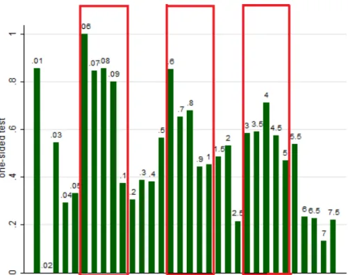
Fig 6shows frequency of use of one-sided tests for different actualpvalues (if one-sided test was to be used), only for the cases when the underlyingt-statistic is given and it is possible to establish whether one- or two-sided test was used. For values below .001, intervals of length .01% were used, for values between .001 and .01: intervals of length .1%, and between .01 and Fig 5. Frequency of reporting directly over intervals of actualpvalue (rounded up).
.075: of length .5%. (The range is restricted for the sake of clarity of the picture, while mixed scale makes the exhibition of the hypothesized effects possible. It also corresponds to the fact that the density of the empirical distribution ofpvalues is decreasing—there would not be enough entries to make inference about very short intervals further away from 0.) For example, the fifth bar on the left shows that some 35% of values between .04% and .05% are reported as one-sided. The red boxes contain these bars that we predicted to be high, because they corre-spond to findings that will be significant at given threshold (.1%, 1%, 5% respectively) only when one-sided test is reported.
Result:The data displays all the hypothesized patterns: Indeed, we see that authors tend to use two-sided tests (overall, of all 1376 cases, one-sided test was only used 35,8% of the time), except for the range of .0005–.0009, .005–.0.008 and .025–.045. These intervals overlap almost perfectly with the intervals on which a one-sided test is significant at .1%, 1% and 5% respec-tively, but a two-sided test is not and thus the use of one-sided test is predicted.
Again, while this is a combined effect of authors’strategizing and publication bias, the latter is unlikely to account for the large part of it.
The choice of precision. Suppose now that the researcher chooses to report thepvalue di-rectly. The data shows that she typically (about 90% of the cases) reports either 2 or 3 decimals. Can we find evidence that the choice which of the two to use is made in a way that makes find-ings appear more significant?
First of all, it would imply that different entries within one paper have different precision. This, of course would not yet prove that the choice of precision is being made strategically. To investigate that issue, we need to focus on these entries where the underlying statistic is given and thus the actualpvalue can be recalculated. We can only consider those cases, where it can be established whether rounding from three to two decimals raised or lowered the number. For Fig 6. Frequency of use of one-sided tests given actual one-sidedpvalues (printed above each bar rather than on the axis and with percent sign omitted for greater readability, rounded up).
example, if we know that the truepvalue falls in the range of (.0795,.08), it will be, when rounded to two decimals (thus to .08), increased. I call such entries“roundable up”. Similarly if the true value is known to be between .13 and .135, it is“roundable down”(to .13). If, however, the interval of possible correctpvalues is e.g. [.17893,18217] then it is neither roundable up nor down because we do not know whether it is smaller or larger than the rounded value of .18. We can now speculate that values that are“roundable up”will indeed be rounded less often than those“roundable down”.
Hypothesis:(Strategic rounding)
1. Precision (number of decimals) will vary within papers
2. Roundable up values will be rounded less often than those roundable down,
3. This discrepancy will be particularly strong at the thresholds
Indeed, I find that researchers are not consistent in their choices of precision within one paper. Suppose for example that three decimals are initially obtained (typically from a statisti-cal package). If these are reported with maximum precision, we expect that about 90% of values reported directly in the paper will have three decimals—the remaining 10% will have 0 as the last digit, thus being likely to be abbreviated to just two decimals. About 9% will have two deci-mals (0 as the last but not second to last digit) and 1% just one decimal.
In fact, only about 61.4% of entries, rather than 90%, have paper-specific maximum preci-sion. Again, this is not about very low values only. If I discard allpvalues lower or equal to .01 and redefine the maximum precision, I find that still just 66% of entries achieve it.
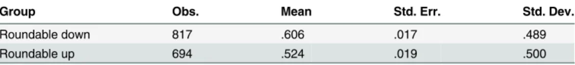
Regarding (2), we can see inTable 2that the option to round is used 60.6% of the time if it lowers the original value (roundable down) and only 52.4% of the time if it raises it (roundable up) (All the actualpvalues below .01 have been discarded for this calculation, as it may be more natural to round (up to .01) values like .008 than to round (down to 0) values such as .003.;values above. 99 were left out for the same reason). The difference is significant,p= .001 (two-sidedt-test) when individualpvalue is used as unit of observation. As the referees and the editor rightly pointed out, this result must be treated with caution because in principle values within one paper are not independent. The alternative approach would be to treat one paper as one observation and then even that only if it satisfies three conditions: 1) at least one round-able-up, 2) at least one roundable-down, 3) different fractions of actually rounded values for these two categories. The results are similar to those onpvalue level in that 54% of such papers have more rounding in case of roundable-downs than roundable-ups (p= .05).
Further analysis revealed that the effect is partly driven bypvalues around the 5% threshold. Roundable down values just above it, between .050 and .055 are rounded down more than 60% of the time, while those in the neighboring range .055-.060 are rounded (up) less than 40% of the time (p= .01, again under the assumption of independent observations).
Interestingly, values just below the intervals, i.e. values in .005-.01 and .0045-.05 have lowest overall probabilities of being actually rounded up. This partly accounts for the left part of the
Table 2. Actual rounding in roundable downs and roundable ups.
Group Obs. Mean Std. Err. Std. Dev.
Roundable down 817 .606 .017 .489
Roundable up 694 .524 .019 .500
H0: diff = 0, Ha: diff! = 0; t = 3.192, P>|t| = 0.001.
structure around 5% visible inFig 1. For example, values from the (.40,.45) interval are more often rounded than the values from the (.45,.50) interval.
Again, it is not logically impossible to exclude an alternative explanation of the fact that op-portunities to round down seem to be taken more often than opop-portunities to round up; it could simply result from the publication bias—selection on reportedpvalues—because round-ing down increases publication chances and roundround-ing up hurts them. However, such an effect would have to be extremely strong to account for the data. To acknowledge this, we may do a little exercise. It will show just how powerful the publication bias would have to be to explain the discrepancy between rounded ups and rounded downs forpvalues in the (.02, .03) range, seeTable 3.
Let us first carefully consider where our sample of, say,pvalues actually rounded down to .02 (there are 59 of them) precisely come from. Among the population of allpvalues that come out of statistical analyses in studies submitted to our journals, they have to satisfy four condi-tions in order to be observed as“rounded down to .02”. That is, they must:
a. indeed be in the interval of .020-.25
b. be reported using the equality sign rather than by comparison with a threshold
c. be actually rounded (down) rather than reported with three or more decimals
d. be in an accepted paper, given rounding (I make a conservative simplifying assumption here that only the reported, not the underlying truepvalue affects the probability of publication).
Let us denote the probabilities involved in points c. and d. asP(RD) andP(acc|.02) respec-tively. Similarly, to be included in our sample of roundable downs within the same interval that havenotbeen rounded,pvalues must satisfy a. and b. as above and additionally c’.: benot
rounded and d’.: be in an accepted paper, givennorounding. The relevant probabilities will be 1-P(RD) andP(acc|.020-.025). Using the numbers given inTable 3we thus conclude that
PðRDÞ 1 PðRDÞ
Pðaccj:02Þ
Pðaccj:020 :025Þ¼59=58:(Note that the probabilities associated with points a. and b. cancel out and thus are irrelevant). The second fraction is a measure of publication bias for this range.
Similarly, for the values in the (.025,.30) interval we infer that PðRUÞ 1 PðRUÞ
Pðaccj:03Þ
Pðaccj:025 :030Þ¼41=70; wherebyP(RU) refers to the probability of rounding up of apvalue that lies within (.025,.30). If we now supposed that authors are equally eager to round up as down,P(RU) =P(RD), it would lead to the conclusion that Pðaccj:02Þ
Pðaccj:020 :025Þ
Pðaccj:025 :030Þ Pðaccj:03Þ ¼
59=58
41=701:74:Thus the combined ef-fect of two shifts of a singlepvalue by less than half a percentage point (from .03 to somewhere between .025 and .03 and from somewhere between .02 and .025 to .02) would have to increase the probability of publication by 74%. Such an extreme publication bias is highly implausible.
Strategic mistakes?. In this subsection I investigate the cases in which the recalculatedp
values are inconsistent with the reported ones. To begin with, these instances are fairly com-mon. The reportedpvalue falls outside the permissible range (in which it should be given the value of the underlying statistic) 9.2% of the time.
Table 3. Rounded and not roundedpvalues in the (.02-.03) interval.
Rounded Not rounded Total
Roundable down (.020-.025) 59 (50.4%) 58 (49.6%) 117
Roundable up (.025-.030) 41 (36.9%) 70 (63.1%) 111
To make it clear, generally speaking we cannot know which part is erroneous—the p value, the test-statistic or perhaps the number of degrees of freedom (df). An anonymous referee made an interesting and plausible suggestion that authors may be particularly likely to misre-port the latter. The referee also pointed out that such possibility may be explored by calculating how many discrepancies could be explained by replacing the (possibly incorrectly) reported df with some other integer. I have run a simulation for all the errors involvingχ2statistics and di-rectly reportedpvalues, with“alternative”df values running from 1 to 1000 (less than 1% ofχ2 statistics in my sample have even higher df). It turns out that in 76.8% of these entries reported
pvalue would not be correct for any df. It thus appears that only a small minority of errors could have arisen because only the df was misreported. A similar exercise could be done forF
andtstatistics, the additional complication being that in the former we would have to allow in simulations for errors in both d1 and d2 and in the latter—for tests being one- or two-sided.
Another explanation of the high number of mistakes, also suggested by the referee, is that authors may inadvertently paste the samepvalue twice (i.e. by mistake report the figure corre-sponding to another test). To verify how often this may be happening I have created variable
“repetition”taking value of 1 if and only if the samepvalue, greater than .01, is reported direct-ly (i.e. using equality sign) more than once in the same paper. It indeed turns out to be a power-ful predictor—a whooping 24.9% of such entries are inconsistent. However, because they only constitute 3.7% of all entries, error rate in not-repetitivepvalues remains very high, equal to 8.8%.
Given that a substantial number of discrepancies seem to be due to misreportedpvalues, I further hypothesize that researchers are more eager to double-check when the value to be re-ported is not to their liking, i.e. implies non-significance. As a result, remaining mistakes would more often than not be self-serving. To verify this hypothesis I investigate how often the reported value is higher than the actual value rather than lower, for each interval of length .01 separately. Inspection ofFig 7yields interesting observations (note that for clarity of the picture only first 25 intervals are considered.) We note that a mistake typically leads to lower, not higher values: the mean of mistake decreases is substantially above .05 for most intervals, in particularallthe intervals below the 10% threshold. This is perplexing. As a matter of fact we initially had reasons to expect that most mistakes should lead to reported values beinghigher
than true values, at least in the case of low true values. First, there is more“space”for mistakes leading to higher reported value. For example if incorrectly reported values were distributed uniformly, there should be, e.g. just a chance of .054 for the incorrectly reportedpvalue to be lower than the original value of .054. Given that most correctpvalues are low, large majority of mistakes would involve over-reporting. Second, the“typical”mistake that I find in the data rel-atively frequently, i.e. omission of the initial“0”(thus turning .067 into. 67 etc.) necessarily leads to the reportedpvalue being higher than the true one.
We also see that largest discrepancy between the two types of mistakes is for the sixth inter-val, where rounding down is most desirable.
Arguably, most mistakes do not lead to great misrepresentation of the data. For example, the medianpvalue among the entries wrongly reported as“p<.05”is 0.066. Still, for about 25% of these cases the truepvalue exceeds .1, thus is two times higher than the reported threshold; the mean is equal to .144. Given that mistakes are not extremely frequent and that they some-times lead to substantial changes in thepvalue, the fact that most of them lead to lower, not higherpvalues, may have well resulted chiefly from selection (publication bias). In other words, I cannot prove that authors selectively overlook mistakes that happen to lower theirp
As mentioned before, a discrepancy could also arise from thepvalue being correct but the underlying statistic (its value or number of degrees of freedom) being wrong. Under the as-sumption that it is thepvalue is what attracts most attention, we may expect that such errors are equally likely to go either way. This observation thus only sthrengthens the result.
As pointed out by a referee, it seems instructive to look at the number of mistakes per paper. This distribution is reported inTable 4. It is somewhat reassuring that more than three-quar-ters of papers are error-free (or almost 90% if we ignore very small mistakes that do not change the second decimal) and papers with very many mistakes are rare On the other hand, note that on average we only have 5.08 entries per paper for which we can re-calculatepvalue from the underlying test-stastic and tell if the reported figure is consistent or not. As a result fractions of mistakes remain high, e.g. one in ten papers has at least one-third of its statistics wrong. Fig 7. Fraction of mistakes leading to the reportedpvalue being lower rather than higher than the actualpvalue, over the calculatedpvalue (rounded up, percent sign omitted).
doi:10.1371/journal.pone.0127872.g007
Table 4. Distribution of number of mistakes per paper.
Number of mistakes # of papers % Cum. %
0 4101 78.59 78.59
1 613 11.75 90.34
2 236 4.52 94.86
3 113 2.17 97.03
4 53 1.02 98.05
5 34 0.65 98.70
6–10 54 1.03 99.73
11–26 14 .27 100.00
TOTAL 5218 100
Discussion and Conclusions
Upon analyzing thepvalues and underlying F, t andχ2reported in top journals in experimen-tal psychology I find some disturbing patterns. One interpretation that correctly organizes these findings is that the authors, being aware of that or not, tend to use their“degrees of free-dom”to their advantage, rather than follow any predetermined best practice. In particular, they seem to engage into strategic choice of sign and threshold, strategic choice between one-sided and two-one-sided tests and strategic rounding. Reportedpvalues are surprisingly often in-consistent with the underlying (reported) statistic and these mistakes tend to lower thepvalue.
Without obtaining the original data and re-running all the estimations (which of course could only be done with a much smaller sample) we cannot identify other mistakes or ques-tionable practices. We do however observe an intriguing bi-modality in the distribution ofp
values: next to the mode situated close to 0 we also have a bump centered near the significance threshold of .05. The left part of the bump—“extra”values just below the significance thresh-old, is not fully explained by any of the identified patters in the way thepvalues are reported. Therefore it persists (in the form of flatter density curve) also in the distribution of the actualp
values, re-calculated from the underlying statistics. One possible explanation is based on the general assumption that researchers recognize and strategically react to the publication bias. It has to be stressed that the analysis presented above is rather novel and exploratory and perhaps poses more questions than it can answer. For example, I have no means to distinguish between the "crucial" and the "control" variables. Nor can we tell between manipulation checks (that tend to be highly significant) and treatment effects. Further, on some rare occasions, the null result can actually be desirable (e.g. when a control treatment is compared to past experi-ments to rule out the possibility that the current subject pool is highly unusual) which could re-sult in the opposite tendencies in reporting. In this sense the effects would have probably been stronger had I been able to focus solely on“central”variables. In any case it may be a useful ex-ercise to look for alternative explanations of the observed patterns.
The analysis may also be expanded in many interesting directions. For example, one could try to identify the "strategic reporters" to verify whether they are consistently inconsistent in different papers.
In any case, if my findings prove to be robust and putative interpretations broadly correct, they have significant implications. They seem to support the proposal to“redefine misconduct as distorted reporting”[31].
They generally call for more discipline in research, more robustness checks and more repli-cations. As Dewald and others [32] assert "(. . .) errors in published articles are a commonplace
rather than a rare occurrence". In the field of psychology in particular the concern for repro-ducibility of findings has been growing in the last years [33]. My findings also indicate that ex-panding study pre-registration to social sciences could be a good idea (see [34] and other papers in the Winter 2013 volume ofPolitical Analysis). They further suggest the referees should look more carefully at the reported statistics, ask for raw data and inspect it carefully. Incidentally, even the revision process of this very paper involved at least two obvious mistakes on my part being found by the referees and surely many readers had similar experience.
thresholds altogether [39]. My findings about the adverse incentive effects of the standard use of the significance thresholds indicate that these suggestions should be taken seriously.
Author Contributions
Conceived and designed the experiments: MK. Performed the experiments: MK. Analyzed the data: MK. Contributed reagents/materials/analysis tools: MK. Wrote the paper: MK.
References
1. Simmons JP, Nelson LD, Simonsohn U (2011) False-positive psychology: Undisclosed flexibility in data collection and analysis allows presenting anything as significant. Psychological Science 22: 1359–1366. doi:10.1177/0956797611417632PMID:22006061
2. Nosek BA, Spies JR, Motyl M (2012) Scientific Utopia II. Restructuring Incentives and Practices to Pro-mote Truth Over Publishability. Perspectives on Psychological Science 7(6): 615–631.
3. Sterling TD, Rosenbaum WL, Weinkam JJ (1995) Publication decisions revisited: the effect of the out-come of statistical tests on the decision to publish and vice versa. American Statistician 49(1): 108–
112.
4. Stanley TD (2005) Beyond Publication Bias. Journal of Economic Surveys 19(3): 309–345. 5. Dwan K, Altman D G, Arnaiz J A, Bloom J, Chan A W, Cronin E, et al. (2008) Systematic review of the
empirical evidence of study publication bias and outcome reporting bias. PloS one, 3(8), e3081. doi: 10.1371/journal.pone.0003081PMID:18769481
6. Ferguson C, Heene M (2012) A Vast Graveyard of Undead Theories Publication Bias and Psychologi-cal Science’s Aversion to the Null. Perspectives on Psychological Science 7(6): 555–561.
7. Iyengar S, Greenhouse JB (1988) Selection models and the file drawer problem. Statistical Science 3: 109–117.
8. Wolf PK (1986) Pressure to publish and fraud in science. Annals of Internal Medicine 104(2): 254–6. PMID:3946955
9. Steneck N (2006) Fostering Integrity in Research: Definitions, Current Knowledge, and Future Direc-tions. Science and Engineering Ethics 12: 53–74. PMID:16501647
10. Fanelli D (2009) How many scientists fabricate and falsify research? A systematic review and meta-analysis of survey data. PLOS one 4: e5738. doi:10.1371/journal.pone.0005738PMID:19478950 11. Martinson BC, Anderson MS, de Vries R (2005) Scientists behaving badly. Nature 435: 737–8. PMID:
15944677
12. John LK, Loewenstein G, Prelec D (2012) Measuring the prevalence of questionable research practices with incentives for truth telling. Psychological science 23(5): 524–532. doi:10.1177/
0956797611430953PMID:22508865
13. Wagenmakers E-J (2007) A practical solution to the pervasive problems of p values. Psychonomic Bul-letin & Review 14(5): 779–804.
14. Kerr NL (1998) HARKing: Hypothesizing after the results are known. Personality and Social Psycholo-gy Review 2: 196–217. PMID:15647155
15. Leamer EE (1983) Let's take the con out of econometrics. American Economic Review 73(1): 31–43. 16. Roth A (1994) Let’s Keep the Con out of Experimental Economics. A Methodological Note. Empirical
Economics 19: 279–289. PMID:7813966
17. Gerber A S, Malhotra N, Dowling C M, Doherty D (2010) Publication bias in two political behavior litera-tures. American politics research, 38(4), 591–613.
18. Ridley J, Kolm N, Freckelton RP, Gage MJG (2007) An unexpected influence of widely used signifi-cance thresholds on the distribution of reported P-values. Journal of Evolutionary Biology 20: 1082–
1089. PMID:17465918
19. Ioannidis JPA, Trikalinos TA (2007) An exploratory test for an excess of significant findings. Clinical Tri-als 4: 245–253. PMID:17715249
20. Gerber AS, Malhotra N (2008a) Do Statistical Reporting Standards Affect What Is Published? Publica-tion Bias in Two Leading Political Science Journals. Quarterly Journal of Political Science 3: 313–326. 21. Gerber AS, Malhotra N (2008b) Publication bias in empirical sociological research—Do arbitrary
signifi-cance levels distort published results? Sociological Methods & Research 37: 3–30.
23. Bakker M, Wicherts JM (2011) The (mis)reporting of statistical results in psychology. Behavior Re-search Methods 43(3): 666–678. doi:10.3758/s13428-011-0089-5PMID:21494917
24. Leggett N C, Thomas N A, Loetscher T, Nicholls M E (2013) The life of p:“Just significant”results are on the rise. The Quarterly Journal of Experimental Psychology, 66(12), 2303–2309. doi:10.1080/ 17470218.2013.863371PMID:24205936
25. Masicampo EJ, Lalande DR (2012) A peculiar prevalence of p values just below .05. The Quarterly Journal of Experimental Psychology 65(11): 2271–2279. doi:10.1080/17470218.2012.711335PMID: 22853650
26. Fanelli D (2010)“Positive" results increase down the Hierarchy of the Sciences. PLoS ONE 5(3): e10068 doi:10.1371/journal.pone.0010068
27. Hung H J, O'Neill R T, Bauer P, Kohne K (1997) The behavior of the P-value when the alternative hy-pothesis is true. Biometrics, 11–22.
28. Simonsohn U, Nelson L D, Simmons, J P (2013) P-Curve: A Key to the File-Drawer. Journal of Experi-mental Psychology: General, Jul 15.
29. Cox DR (1966) Notes on the analysis of mixed frequency distributions. British Journal of Mathematical Statistical Psychology 19: 39–47.
30. Good IJ, Gaskins RA (1980) Density estimation and bump-hunting by the penalized likelihood method exemplified by scattering and meteorite data. Journal of the American Statistical Association 75(369): 42–56. PMID:12263159
31. Fanelli D (2013) Redefine misconduct as distorted reporting. Nature 494(149) doi:10.1038/494149a PMID:23407504
32. Pashler H, Wagenmakers E J (2012) Editors’Introduction to the Special Section on Replicability in Psy-chological Science A Crisis of Confidence?. Perspectives on PsyPsy-chological Science, 7(6), 528–530. 33. Dewald W G, Thursby J G, Anderson RG (1986) "Replication in empirical economics: The journal of
money, credit and banking project." The American Economic Review Vol. 76, No. 4: 587–603. 34. Humphreys M, de la Sierra R S, van der Windt P (2013) Fishing, commitment, and communication: A
proposal for comprehensive nonbinding research registration. Political Analysis, 21(1), 1–20. 35. Cohen J (1994) The Earth Is Round (p<.05). American Psychologist 49(12): 997–1003.
36. Dixon P (2003) Thepvalue Fallacy and How to Avoid It. Canadian Journal of Experimental Psychology 57(3): 189–202. PMID:14596477
37. Davies J B, Ross A (2012) Sorry everyone, but it didn't work (p = 0.06). Addiction Research & Theory, 21(4), 348–355.
38. Sterne JAC, Smith GD (2001) Sifting the evidence—what's wrong with significance tests? British Medi-cal Journal 322: 226–31. PMID:11159626
![Table 1. Distribution of number of “ just significant ” (.045 – .050] and “ almost significant ” (.050 – .055) directly reported p values per paper.](https://thumb-eu.123doks.com/thumbv2/123dok_br/18376113.355849/7.918.297.867.846.1048/table-distribution-number-significant-significant-directly-reported-values.webp)