www.the-cryosphere.net/9/451/2015/ doi:10.5194/tc-9-451-2015
© Author(s) 2015. CC Attribution 3.0 License.
Snow-cover reconstruction methodology for mountainous regions
based on historic in situ observations and recent remote sensing data
A. Gafurov1, S. Vorogushyn1, D. Farinotti1,*, D. Duethmann1, A. Merkushkin2, and B. Merz1
1Department of Hydrology, GFZ German Research Centre for Geosciences, Potsdam, Germany 2Uzbek Hydrometeorological Service (Uzhydromet), Tashkent, Uzbekistan
*now at: Swiss Federal Institute for Forest, Snow and Landscape Research WSL, Birmensdorf, Switzerland
Correspondence to:A. Gafurov ([email protected])
Received: 29 July 2014 – Published in The Cryosphere Discuss.: 1 September 2014 Revised: 6 February 2015 – Accepted: 10 February 2015 – Published: 4 March 2015
Abstract.Spatially distributed snow-cover extent can be de-rived from remote sensing data with good accuracy. How-ever, such data are available for recent decades only, af-ter satellite missions with proper snow detection capabilities were launched. Yet, longer time series of snow-cover area are usually required, e.g., for hydrological model calibration or water availability assessment in the past. We present a methodology to reconstruct historical snow coverage using recently available remote sensing data and long-term point observations of snow depth from existing meteorological sta-tions. The methodology is mainly based on correlations be-tween station records and spatial snow-cover patterns. Addi-tionally, topography and temporal persistence of snow pat-terns are taken into account. The methodology was applied to the Zerafshan River basin in Central Asia – a very data-sparse region. Reconstructed snow cover was cross validated against independent remote sensing data and shows an accu-racy of about 85 %. The methodology can be used in moun-tainous regions to overcome the data gap for earlier decades when the availability of remote sensing snow-cover data was strongly limited.
1 Introduction
Water resources from remote mountain catchments play a crucial role in the development of regions in or in the vicin-ity of mountain ranges (Pellicciotti et al., 2012). Seasonal snow is an important water resource in many of Earth’s semi-arid regions (Durand et al., 2008). Particularly in Central Asia, seasonal snowmelt decisively contributes to the total
runoff volume (Ososkova et al., 2000; Unger-Shayesteh et al., 2013).
Information on snow cover and snow depth and ideally on snow water equivalent in Central Asian catchments is crucial for seasonal forecasts of water availability and for calibration and validation of hydrological models. However, the avail-able sparse station-based data are insufficient to represent the snow-cover variability over the large and remote moun-tain areas (Erickson et al., 2005). The development of remote sensing techniques during recent decades allows the deriva-tion of snow cover spatially (Liu et al., 2012). Widely used remotely sensed snow-cover products are from Advanced Very High Resolution Radiometer (AVHRR), Landsat and Moderate Resolution Imaging Spectroradiometer (MODIS) missions. Whereas AVHRR (launched 1978) and Landsat (launched 1972) offer remote sensing data for a longer pe-riod, MODIS is available only after 2000. However, snow cover from Landsat and AVHRR needs to be derived by the end user themselves, whereas MODIS offers already-compiled snow-cover product. The above-mentioned snow products are extremely useful to study snow cover world-wide; however, they are strongly limited by the presence of clouds. Recently, the reconstruction of snow-cover time se-ries from AVHRR data for Central Asia has been reported by Zhou et al. (2013), but they are also limited in time starting in 1986 at earliest.
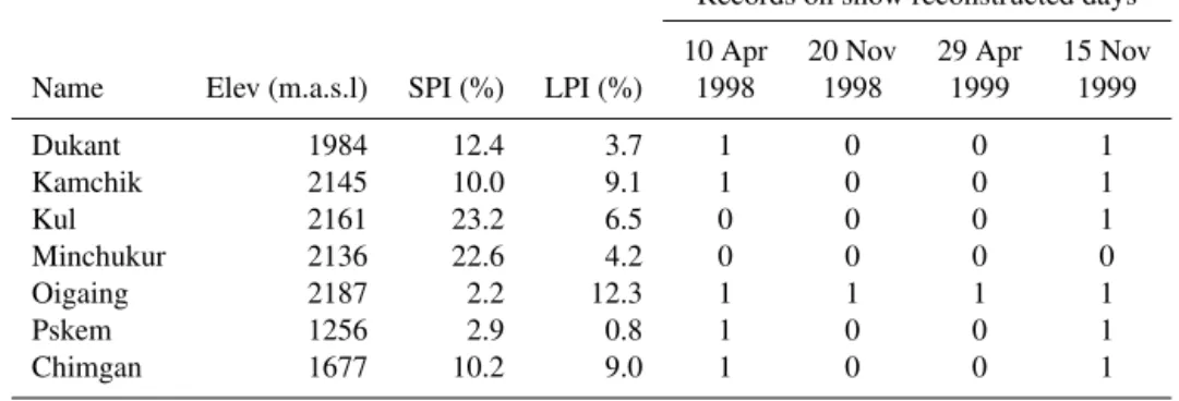
Table 1.Uzhydromet snow observation stations with indication of elevation (Elev), and snow predictability index (SPI) and land predictabil-ity index (LPI) values for the study area (see Sect. 4). The entries “records on snow reconstructed days” indicate whether a station was snow covered (0) or snow free (1) during a day for which snow-cover reconstruction was conducted and Landsat scenes were available for validation.
Records on snow reconstructed days
10 Apr 20 Nov 29 Apr 15 Nov Name Elev (m.a.s.l) SPI (%) LPI (%) 1998 1998 1999 1999
Dukant 1984 12.4 3.7 1 0 0 1
Kamchik 2145 10.0 9.1 1 0 0 1
Kul 2161 23.2 6.5 0 0 0 1
Minchukur 2136 22.6 4.2 0 0 0 0
Oigaing 2187 2.2 12.3 1 1 1 1
Pskem 1256 2.9 0.8 1 0 0 1
Chimgan 1677 10.2 9.0 1 0 0 1
Particularly for hydrological model calibration, spatially dis-tributed snow-cover data offer high information content re-quired to constrain model parameters (Finger et al., 2011; Duethmann et al., 2014).
In Central Asia, continuous hydrometeorological records are widely available from the 1960s and earlier until the col-lapse of the Soviet Union in 1991. In contrast, continuous remote sensing snow-cover data from MODIS are readily available after 2000, when station data are very scarce. We present a methodology which enables reconstructing histor-ical snow-cover pattern using long-term, point-based obser-vations from existing meteorological stations and recent re-motely sensed snow-cover data. By merging high-resolution spatial satellite data with long-term station data, snow-cover patterns can be reconstructed for several decades into the past.
Only a limited number of studies on snow-cover recon-struction have been conducted in the past that use long-term station observations and recent remote sensing data (son, 1991; Brown, 2000; Frei et al., 1999; Brown and Robin-son, 2011). These studies are, however, conducted at the continental scale under conditions of dense station network availability and neglecting the effect of topography. Robin-son (1991) and Frei et al. (1999) conducted reconstruction of snow cover based on regression analysis between snow char-acteristics and snow-cover area (SCA) derived from AVHRR satellite observations. As snow characteristics both studies used snow-cover duration derived from interpolated station records. Another study by Brown (2000) conducted recon-struction of snow cover for “pre-satellite era” interpolat-ing snow-depth data from station network. For grid cells of nearly 200 km, the interpolation of snow cover was done us-ing different thresholds for snow depth and compared against NOAA snow-cover extent during “satellite era”. The cali-bration showed 2 cm to be most appropriate snow depth for accurate snow-cover reconstruction based on station data. Brown and Robinson (2011) updated and extended the
snow-cover reconstruction of Brown (2000) to the period 1922– 2010 and used these data for trend analysis of snow-cover ex-tent in the Northern Hemisphere. These studies can be help-ful in assessing climate-related variations of snow cover but are hardly transferable to smaller catchment scale with mod-erate resolution and limited station data availability.
Different to those studies mentioned above, we present a methodology for snow-cover reconstruction (1) with mod-erate spatial resolution (500 m), (2) suitable for catchment scale hydrological studies, (3) accounting topography and (4) delivering spatially distributed snow-cover maps. The methodology takes advantage of the strong control of topog-raphy on the spatial snow-cover distribution. Hence, mea-surements from snow observation stations at different ele-vations can be interpreted as representative sites to predict snow-cover patterns. The methodology consists of five suc-cessive steps which make use of topographic information and correlations between station records and spatial snow-cover patterns. In order to test the presented methodology, snow-cover reconstruction was conducted for 4 days (Table 1) for which independent Landsat data were available.
2 Study area
The methodology for snow-cover reconstruction was devel-oped and tested for the area containing the upper Zerafshan River basin, Central Asia (Fig. 1).
Figure 1.Location of the upper Zerafshan River basin in the Gissaro-Alai mountain range, Central Asia. Snow-cover reconstruction was conducted for the entire area of Fig. 1b and validated for the area with Landsat footprint.
regimes in Fig. 2. The highest precipitation is brought by westerly flows during winter and spring, with a clear mini-mum during summer and early autumn (Aizen et al., 1995). The highest runoff, however, occurs during summer months and is driven by snow and glacier melt. According to MODIS Landcover product (MCD12Q1) from 2009, the main land cover types in the study area are grasslands (60 %), crop-lands (9 %), open shrubcrop-lands (7 %), woody savannahs (6 %) and permanent snow- and ice-covered areas (5 %).
3 Data
We used (1) daily in situ snow-depth data, (2) daily MODIS snow-cover data, (3) a digital elevation model (DEM) and (4) Landsat data. The first three data sets were used for snow-cover reconstruction whereas Landsat data were used as an independent data set to validate the results.
3.1 In situ snow-depth data
Daily snow-depth data in the period from 1964 to 2012 were available for seven climate stations located at differ-ent elevations (Fig. 1, Table 1). These data contain continu-ous snow-depth measurements including records on no-snow conditions. Snow depth in these stations are recorded at 1 cm threshold depth. The data were provided by Uzbek Hydrom-eteorological Service (Uzhydromet).
Figure 2.Monthly average air temperature (T), cumulative precipi-tation (P), discharge (Q) and SCA dynamics in the Zerafshan basin. T, P and Q means are based on data for the period from 1930 un-til 2008. Daily SCA is for 2004 obtained from MODIS and cloud eliminated using Gafurov and Bárdossy (2009). Temperature (0◦C in January) and precipitation data are from the Pendjkent station (1016 m a.s.l.), and discharge is measured at the Dupuli gauge (see Fig. 1).
3.2 MODIS snow-cover data
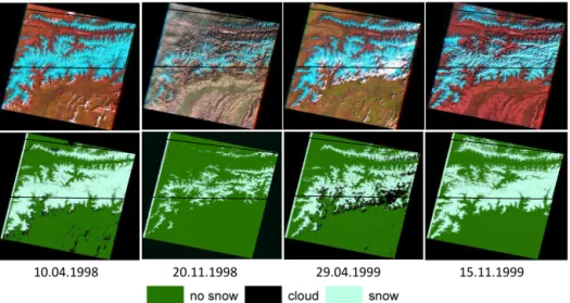
10.04.1998 20.11.1998 29.04.1999 15.11.1999
Figure 3.Original Landsat scenes (top row) and derived snow-cover maps used for validation (bottom row). Black outlines show the valida-tion domain for Zerafshan basin.
normalized difference snow index (NDSI) algorithm (Hall et al., 2002). Its accuracy was tested in different parts of the world showing good agreement with in situ data (Klein and Barnett, 2003; Tekeli et al., 2005; Parajka et al., 2006; Ault et al., 2006; Wang et al., 2008; Liang et al., 2008; Huang et al., 2011; Gafurov et al., 2013; Parajka et al., 2012). The main drawback of MODIS snow-cover data is the limitation due to cloud cover. There have been several studies on fil-tering methods for reducing cloud cover or even removing it completely (e.g., Parajka and Blöschl, 2008b; Gafurov and Bárdossy, 2009; Tong et al., 2009; Hall et al., 2010; Lòpez-Burgos et al., 2013). We used original MODIS snow-cover data to exclude any uncertainty that may be introduced by cloud filtering. The data were obtained from the National Aeronatics and Space Administration (NASA) Earth Observ-ing System Data and Information System (EOSDIS) Reverb platform. MODIS data are distributed as tiles with the size of 10◦×10◦, which makes up a total of 36 horizontal (h) and 18 vertical (v) tiles covering the entire globe. In this study, the tile h23v05, which covers the study area completely, was used.
3.3 Digital elevation model
The void-filled DEM with 90 m spatial resolution from NASA Shuttle Radar Topography Mission (SRTM) was used. SRTM DEM data were obtained from the CGIAR CSI (Consultative Group on International Agricultural Re-search, Consortium for Spatial Information) database (Jarvis et al., 2008). To have the same resolution as the MODIS data (500 m), the 90 m SRTM DEM was aggregated to 500 m. 3.4 Landsat data
Optical remote sensing data from the Landsat Thematic Map-per sensor were used to validate the reconstructed
snow-cover maps. The Landsat data have a spatial resolution of 30 m and a temporal resolution of 16 days. Landsat data from 4 nearly clear-sky days in the snow season (10 April 1998, 20 November 1998, 20 April 1999 and 15 November 1999) were used for validation purposes. Snow-cover maps for the Landsat footprint (see Fig. 1) were prepared using the NDSI methodology. For a detailed description of the algorithm used for deriving snow-cover maps from Landsat refer to Ga-furov et al. (2013). Figure 3 shows raw and processed Land-sat snow-cover maps for the study area.
Since Landsat has a spatial resolution of 30 m and snow reconstruction was performed for 500 m pixels based on MODIS resolution, the processed Landsat snow-cover maps were spatially aggregated to 500 m resolution. This was done by classifying each of the 500 m pixels as snow covered or snow free, based on the majority of the 30 m Landsat pixels within the 500 m pixel.
4 Methodology
elevation-based classifications were used. The methodology consists of five successive steps in which each step estimates a cer-tain fraction of snow cover. This leads to a complete snow-cover reconstruction after step 5. Once the similarities and temporally persistent snow fields are established using exist-ing stations and remote sensexist-ing data, the methodology can be applied to other time periods and is solely based on snow records at meteorological stations. The following five steps are detailed in the next sections:
1. pixel to station CP fields
2. temporally persistent monthly probability fields 3. pixel to pixel CP fields
4. usage of elevation information 5. pixel to station CP for CP<1.
4.1 Pixel-to-station conditional probability
In the first step, we consider the CP of each pixel, given the observed data from a set of snow stations. We compute the CP of each pixel as follows:
Ps(Sx,y|Sn)=
P
(1−ABS(Sx,y,t−Sn,t))
Nx,y
(1)
∀ Sn,t =1,
Pl(Sx,y|Sn)=
P
(1−ABS(Sx,y,t−Sn,t))
Nx,y
(2)
∀ Sn,t =0,
wherePs(Sx,y|Sn)(Pl(Sx,y|Sn))is the CP of a pixel with co-ordinatesxyto be covered by snow (land) given that the sta-tion nalso records snow depth>0 (=0) at the same time.
Sx,y,t andSn,t are binary variables indicating the presence (S=1) or absence (S=0) of snow at pixelxyand stationn
for dayt, respectively.Nx,yis the number of observations si-multaneously available at pixelxy(excluding cloud-covered days) and stationnover the 12 years (2000–2012) for which stationnshowed snow (S=1) or snow-free (S=0) condi-tions. The value of Ps(Sx,y|Sn)(Pl(Sx,y|Sn))varies from 0 to 1, withPs(Sx,y|Sn)=1 (Pl(Sx,y|Sn)=1 ) indicating that a pixel at xy was always observed as snow covered (snow free) in the MODIS data when station n measured snow depth >0 (=0), whilst Ps(Sx,y|Sn)=0 (Pl(Sx,y|Sn)=0) indicates an opposite relationship, i.e., that the MODIS prod-uct at xy always showed snow-free (snow-covered) condi-tions when stationnhad snow depth>0 (=0).
CPs were computed for each MODIS pixel in the study area (total of 169 776 pixels) using over 12 years of avail-able MODIS data and observed snow-depth measurements. Hence, the daily snow-cover maps from MODIS are treated
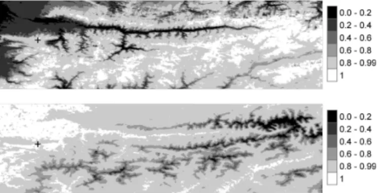
Figure 4.CP maps for snow (top) and land (bottom) conditions of Chimgan station (see Fig. 1) for the study area. The figure shows the same domain as Fig. 1b.
as snow observations for each 500 m grid cell, giving rise to a very dense “observation network”. An example for a CP map for snow and land conditions for Chimgan station is given in Fig. 4. In total, 14 maps were derived (two maps for ev-ery of the seven stations: one forPs(Sx,y|Sn)and one for
Pl(Sx,y|Sn)).
The number of pixels with Ps(Sx,y|Sn)=1 (Pl(Sx,y|Sn)=1) varies from station to station. The higher the number of pixels with Ps(Sx,y|Sn)=1, the higher the predictive power of the station for snow classi-fication is. Similarly, the higher the number of pixels with
Pl(Sx,y|Sn)=1, the higher the predictive power of the sta-tion to predict snow-free condista-tions is. In order to quantify the predictive power of each station, we introduce two terms: snow predictability index (SPI) and land predictability index (LPI). These terms give the fractions of the reconstruction domain with Ps(Sx,y|Sn)=1 for a given station for snow and land conditions, respectively:
SPIn=
P
(Ps(Sx,y|Sn)=1)
N ·100 [%], (3)
LPIn=
P
(Pl(Sx,y|Sn)=1)
N ·100 [%], (4)
where SPInand LPIn are the snow predictability index and the land predictability index of stationn, respectively.N is the total number of pixels (169 776) in the entire study area. Pixels withPs(Sx,y|Sn)=1 in Fig. 4 (top) add up to 10.2 %, which is the SPI value of the Chimgan station for the entire domain. This means that when the Chimgan station shows a snow depth above zero, 10.2 % of the study area can be classified as snow covered as well. Pixels withPl(Sx,y|Sn)= 1 in Fig. 4 (bottom) add up to 9.0 %, which means that when the Chimgan station shows snow-free conditions, 9.0 % of the study area can be assigned as snow free.
u
n
d
e
f.
s
n
o
w
la
n
d
Figure 5.Temporally persistent spatial snow (MPs=1) and land (MPl=1)patterns for April in the study area shown in Fig. 1b. Pixels with “undef” indicate MPs<1 or MPl<1, for which classification is not possible in this step.
elevation far higher than the elevation of Chimgan station tend to be snow covered if Chimgan station records positive snow depth, whilst pixels with an elevation far below the el-evation of Chimgan station tend to be snow free if Chimgan station records snow depth of zero. Table 1 shows the SPI and LPI values for each station. The stations Kul and Minchukur near the Zerafshan basin (see Fig. 1) have the highest SPI val-ues (23.2 and 22.6 %, respectively). Other stations, located further away from the catchment, have smaller SPI values. Noticeably, Oigaing station, located farthest away from the Zerafshan basin, has the highest LPI value (12.3 %). This can be explained by the high elevation of the station. When the station indicates snow-free conditions, pixels with sig-nificantly lower elevation are likely to be snow free as well. Assuming that the dependencies remain stable in time, the computed CPs of each pixel can be used to classify indi-vidual pixels for any arbitrary day prior to the availability of MODIS data (before 2000) for which station records are available:
Sx,y,t =1 if Ps(Sx,y|Sn)=1 andSn,t =1, (5)
Sx,y,t =0 if
Pl(Sx,y|Sn)=1 andSn,t=0
. (6)
This step leads to a partially reconstructed snow-cover map which is further enhanced in the next steps.
4.2 Monthly probability fields
Snow-cover extent is a seasonally variable parameter. Ac-cordingly, the probability of a certain pixel to be covered by snow or land varies with time. The second step for re-constructing snow cover is based on the observation that during different months, certain pixels are snow covered or snow free with high confidence. The spatial distributions of such temporally persistent patterns can be identified using the available MODIS snow-cover data in the period 2000–2012. A monthly probability (MP) of each pixel to be covered by snow or land in a certain month is computed according to
MPsx,y,m= P
(S(x,y,t ), (t∈m)=1)
Nx,y,m
, (7)
MPlx,y,m=
P
(S(x,y,t ), (t∈m)=0)
Nx,y,m
, (8)
where MPsx,y,m and MPlx,y,m are the probabilities of pixel
xyto be covered by snow or land in monthm, respectively.
S(x,y,t )indicates the coverage (snow or land) of pixelxyon dayt.Nx,y,mis the total number of MODIS observations of pixelxy and monthmin the period 2000–2012. The maxi-mum value of MPsx,y,m(MPlx,y,m) is 1, meaning that the pixel
xy was covered always by snow (land) in monthmduring the cloud-free days in the period 2000–2012. Computation of MPs for every pixel in the study area leads to MP maps for all 12 months as illustrated exemplarily in Fig. 5 for April.
Pixels with MPsx,y,m=1 in Fig. 5, i.e., pixels that were al-ways snow covered in April, add up to 12.7 % of the whole area. This means that 12.7 % of the study area can be classi-fied as snow covered in April. Pixels with MPlx,y,m=1 add up to 14.9 %, i.e., 14.9 % of the domain can be classified as snow free in April. To remain consistent with the termi-nology used in the first step, we call the sum of pixels with MPsx,y,m=1 (MPlx,y,m=1) the monthly SPI (LPI) value for snow (land). Monthly SPI and LPI are defined in a similar way as in step 1 (Eqs. 3 and 4).
The main idea in this step is to transfer these temporally persistent monthly spatial snow/land patterns (SPIm/LPIm) to the past to reconstruct historical snow cover. However, the validity of these temporally persistent spatial snow/land pat-terns over a longer time in the past is not assured due to, e.g., potential warmer/cooler or wetter/dryer climate conditions. In order to account for possible climatic variability, we intro-duce a buffer as vertical elevation shift from month-specific minimum snow and maximum land lines. We define a month-specific minimum snow line (Hmins ,m)and a month-specific maximum land line (Hmaxl ,m)as
Hmins ,m=min Hx,y ∀ MPsx,y,m=1, (9)
Hmaxl ,m=max Hx,y ∀ MPlx,y,m=1, (10) whereHx,yis the elevation of the pixelxy.Hmaxl is thus the
Table 2. Monthly SPI, LPI,Hmins ,m and Hmaxl ,m values for the study region.
SPI LPI
Month Fraction (%) Hmins Fraction (%) Hmaxl
1 10.1 1544 0.0 658
2 11.4 1164 0.0 2233 3 24.0 1658 0.4 2923 4 12.7 2354 14.9 3323 5 1.1 2900 32.7 3707 6 0.0 3568 49.5 4387 7 0.0 5402 66.3 4434 8 0.0 5402 78.3 4520 9 0.0 4285 51.2 4330 10 0.2 3405 25.3 4089
11 0.9 2750 0.4 2581
12 8.5 2373 0.0 1707
m. Note that below the altitudeHmaxl not all pixels necessar-ily have MPl
x,y,m=1. Similarly,Hmins is the minimum
eleva-tion of all pixels with MPsx,y,m=1 in monthm. Again,Hmins
does not necessarily represent the elevation above which all pixels have MPsx,y,m=1. Table 2 lists monthly SPI and LPI values as well asHmins ,mandHmaxl ,mvalues for the selected area.
These Hmins ,m, Hmaxl ,m and monthly SPI/LPI maps were used to further reconstruct the snow cover resulting from step 1:
Sx,y,t =1 (11)
if Hx,y> Hmins ,m+buffer and MP s
x,y,m=1
t∈m,
Sx,y,t =0 (12)
if Hx,y< Hmaxl ,m−buffer and MPlx,y,m=1
t∈m,
where “buffer” is a parameter accounting for the possible vertical shift in snow line. In order to account for climate variability not represented by the period for which satellite observations are available, “buffer” was set to 500 m. Due to the absence of historical data on snow-line variations in the region, the buffer was estimated corresponding to the maximum observed variation in the equilibrium line altitude (ELA) of Abramov glacier (Table 3, see Fig. 1 for location) for the period 1972–1998 (WGMS, 2001; Pertziger, 1996) and is thus a conservative estimate for the variations in snow line for the study area.
4.3 Pixel-to-pixel conditional probability
In step 1, CPs of each pixel in accordance to station records were computed, and any pixel that hadPs(Sx,y|Sn)=1 was
Figure 6.CP maps for snow (top) and land (bottom) conditions for the pixelx=100,y=100 (black cross) with elevation 2206 m a.s.l.
classified according to the station record. The idea behind the third step is similar, but CPs of each pixel in accordance to other pixels are computed this time. In such a way, the state of different pixels is used as a predictor for snow cover elsewhere. We define the CP of any pixel with coordinates
xyto be covered by snow (land) given that another pixelij
is covered by snow (land) as follows:
Ps(Si,j|Sx,y)=
P
(1−ABS(Si,j,t−Sx,y,t))
Ni,j
(13)
∀ Sx,y,t=1,
Pl(Si,j|Sx,y)=
P
(1−ABS(Si,j,t−Sx,y,t))
Ni,j
(14)
∀ Sx,y,t=0,
whereSi,j,t indicates whether the pixel with coordinatesij is snow covered (S=1) or snow free (S=0) for a given day
t andNi,j is the total number of valid observations (clear sky, no cloud) at pixelijsimultaneously available for a given condition (S=1 orS=0) in the period 2000–2012.
The computation of Ps(Si,j|Sx,y) and Pl(Si,j|Sx,y) ac-cording to Eqs. (13) and (14) is repeated in an “all-versus-all” procedure, which means that all possible combinations of (xy)and (ij) are considered. For the region of interest, this yields at maximum 339 552 (double the total number of pixels) CP maps (i.e., two maps for every pixel: for snow and land condition). However, not all of these maps were used for snow reconstruction since some pixels may have no perfect dependence (no pixels with CP=1) to any other pixel in the study area. An example of the CP maps for snow and snow-free conditions for the pixel located atx=100 andy=100 is given in Fig. 6.
The pixel with coordinates x=100, y=100 has
Ps(Si,j|S100,100)=1 for 30 684 (18 %) other pixels in the
Table 3.ELA records of Abramov glacier (WGMS, 2001; Pertziger, 1996).
Year 1972 1977 1987 1988 1989 1990 1991 1992 1993 1994 1995 1996 1997 1998
ELA
4020 4393 4130 4170 4200 4220 4242 4110 4120 4250 4240 4163 4440 4130 (m a.s.l)
pixel is 18 %, and this can be interpreted as the predictive power for snow of the pixel for the entire study area. Analo-gously, 23 770 pixels (14 %) havePl(Si,j|S100,100)=1 with
this pixel and the LPI value of this pixel is 14 %. The SPI and LPI values of each pixel are derived through Eqs. (3) and (4) and illustrated in Fig. 7 for all pixels in the study area.
The maximum SPI value (Fig. 7, top) is 46 %, meaning that, according to the observations of the period 2000–2012, 46 % (78 189 pixels) of the study area was always snow cov-ered when that particular pixel was snow covcov-ered. The max-imum LPI value (Fig. 7 bottom) is 88 %, meaning that this particular pixel is able to predict snow-free conditions for 88 % (149 685 pixels) of the basin. These two pixels with maximum SPI and LPI values are located within an area which has high predictive power for snow and land, respec-tively. When interpreting Fig. 7, three further features are worth noting: (1) pixels with SPI=0 or LPI=0 exist as well, but these pixels have no predictive power and are there-fore not used in the snow-cover reconstruction; (2) SPI and LPI maps generally reflect the topography of the catchment: lower elevation pixels have higher SPI values and pixels at higher elevations have higher LPI values; (3) snow-free pix-els are easier to predict than snow-covered ones.
The SPI and LPI maps were used for classifying pixels that are still undefined after the previous steps:
Si,j,t=1 if Ps(Si,j|Sx,y)=1 andSx,y,t=1
, (15)
Si,j,t=0 if
Pl(Si,j|Sx,y)=1 andSx,y,t=0
. (16)
Since in this step SPI and LPI maps were generated for every pixel in the basin, this step tends to classify a signifi-cantly larger area than the first step where only seven stations were used for constructing CPs.
4.4 Snow-cover estimation using elevation information from neighboring pixels
This step is adapted from Gafurov et al. (2009) and is based on the information of neighboring pixels. Let us consider a pixel that has not been classified as snow covered or snow free in any of the previous steps. If any of the adjacent eight pixels is covered by snow and the elevation of that snow-covered pixel is lower than the pixel that is still undefined, then the undefined pixel is classified as snow covered. The same idea is applied for snow-free pixels. Hence, this step
Figure 7.SPI (top) and LPI (bottom) values of each pixel (in %) in the study area defined in Fig. 1b.
can be formalized as follows:
Sx,y,t=1 if Sx+k,y+k,t=1 (17)
andHx+k,y+k< Hx,y k∈(−1,1),
Sx,y,t=0 if Sx+k,y+k,t=0 (18)
andHx+k,y+k> Hx,y k∈(−1,1).
This step takes only elevation of neighboring pixel into ac-count. However, in areas where factors others than elevation have an influence on neighboring pixel condition (e.g., pixels located near to water surfaces or forests), additional informa-tion such as a land cover map could be introduced into this step.
4.5 Snow-cover estimation with CP <1
In the last step, thePs(Sx,y|Sn)andPl(Sx,y|Sn)values cal-culated in step 1 are used again. Whereas in step 1 only CP=
Table 4.Contingency table (in %) for the reconstructed snow-cover maps validated against four aggregated Landsat snow-cover images. Four cases are distinguished: SS, LL, SL and LS. The first (second) letter indicates the classification according to the presented algo-rithm (Landsat). “S” stands for snow and “L” for land. “Total” in-dicates the percentage of pixels classified after each step. Results refer to the Landsat domain (dashed line) shown in Fig. 1b.
Day Step SS LL SL LS Total
1 8.5 7.2 0.0 0.0 15.7 10 Apr 2 13.0 14.9 0.1 0.1 28.1 1998 3 17.5 27.1 0.8 0.1 45.5 4 20.6 29.3 1.3 0.2 51.4 5 43.4 42.3 12.5 1.8 100.0
1 0.1 11.2 0.0 0.0 11.3 20 Nov 2 0.2 11.3 0.0 0.0 11.5 1998 3 0.5 30.5 0.0 0.0 31.0 4 1.4 33.4 0.0 0.1 34.9 5 18.1 67.0 2.2 12.7 100.0
1 0.1 13.9 0.0 0.0 14.0 29 Apr 2 7.6 21.5 0.0 0.5 29.6 1999 3 9.0 35.2 0.1 0.7 45.0 4 11.0 38.1 0.3 0.9 50.3 5 24.5 58.8 14.3 2.3 100.0
1 18.4 4.1 0.0 0.4 22.9 15 Nov 2 18.4 4.2 0.0 0.4 23.0 1999 3 24.8 15.7 0.4 0.8 41.7 4 28.5 18.3 0.7 1.3 48.9 5 41.7 42.0 11.2 5.1 100.0
(CI) of each CP. As the CP estimates follow a binomial dis-tribution, we compute lower bound CI of CP according to CIlow(Ps(S
x,y|Sn)) (19)
=Ps Sx,y|Sn
−z
s
1
Nx,y
Ps(S
x,y|Sn)(1−Ps(Sx,y|Sn)),
CIlow(Pl(S
x,y|Sn)) (20)
=Pl Sx,y|Sn−z
s
1
Nx,y
Pl(S
x,y|Sn)(1−Pl(Sx,y|Sn)),
where CIlow(Ps(S
x,y|Sn)) and CI low
(Pl(S
x,y|Sn)) are lower bound of 95 % CI of CP for snow and land conditions, respectively.z
is the constant for 95 % confidence level (1.96). The com-puted lower bound CI for each CP will help to classify still-undefined pixel coverage based on highest confidence level for P Sx,y|Sn
<1 case among 14 CPs. Thus, we use the highest lower bound CI among all CPs of this particular pixel
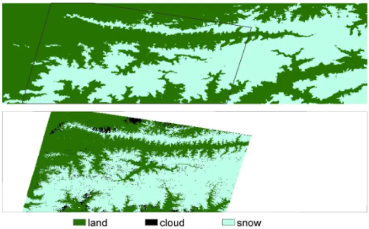
Figure 8.Reconstructed (top) and Landsat (bottom) snow-cover maps for 10 April 1998.
to be decisive for reconstruction.
Sx,y,t=1 if max
CIlow(Ps(S x,y|Sn))
(21)
>maxCIlow(Pl(S x,y|Sn))
n∈1:7
Sx,y,t=0 if max
CIlow(Pl(S x,y|Sn))
(22)
>max
CIlow(Ps(S x,y|Sn))
n∈1:7
Taking maximum lower bound CI values for still-undefined pixels in the last step allows us to complete the classification for all pixels. However, since in this step
P (Sx,y|Sn) <1 was considered, the reconstruction is sub-ject to uncertainty that stems from non-perfect agreement be-tween station records and a pixel in the period 2000–2012.
5 Results and discussion
CI (snow)
0,99 0,50
CI (land)
0,99 0,48
Steps 1-4
land snow
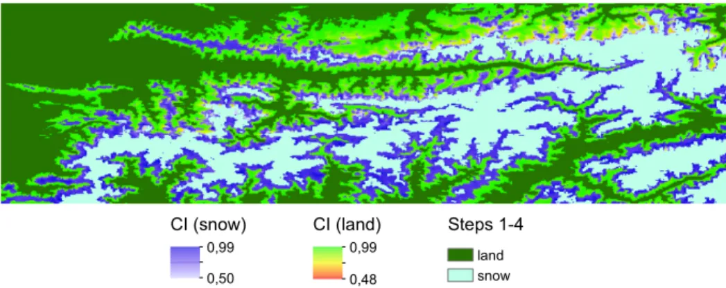
Figure 9.Fraction of reconstruction in steps 1–4 and maximum CI values for snow and land in step 5 for the study area illustrated in Fig. 1b.
As an example, Fig. 8 shows the reconstructed and Landsat-derived snow-cover maps for 10 April 1998. The comparison of these maps results in 85.7 % of correct recon-struction (cases SS+LL in Table 4) and 14.3 % of erroneous reconstruction (SL+LS). Steps 1–4 show high accuracy with only little erroneous reconstruction (ER) whereas step 5 has the lowest accuracy in all validation days. However, the reconstruction fraction (RF) is very high in step 5 compared to previous steps. Note that ER may also be enhanced by er-roneous snow-cover estimation from raw Landsat data and due to the spatial aggregation of Landsat 30 m original reso-lution to 500 m. Another potential bias may come from sim-ilar approaches (NDSI) used to map snow cover both for MODIS snow-cover maps, which are used to assess CPs between station and pixels, and Landsat snow-cover maps, which are used to validate reconstructed snow-cover maps. However, different threshold values than MODIS were used to map snow cover from Landsat, assuring best visual vali-dation of snow and snow-free surface cover.
In order to better illustrate snow reconstruction in step 5, Fig. 9 shows the areal fraction for which the reconstruction was performed in steps 1–4 and maximum lower bound CI obtained in step 5 under CP<1 condition for the validation day of 10 April. Most of the still-unclassified pixels after steps 1–4 have CI values close to 1 and only few pixels have a lower CI value (reddish and light blue colors in Fig. 9). Figure 10 illustrates the trade-off between RF and ER as a function of lower bound CI in step 5. For example, for the validation day of 10 April, ER from steps 1–4 adds up to 1.5 % (Table 4) and RF to 51.4 % (snow and land classes in Fig. 9). With decreasing CI, RF increases but at the cost of an increased ER. However, Fig. 10 also shows that RF is rela-tively high until about CI=0.9 with increasing ER. On all 4 days used for validation, an almost complete reconstruction is achieved with CI>0.9.
Figures 8, 9 and 10 also demonstrate that the methodology provides two types of results for snow-cover reconstruction: deterministic and probabilistic snow-cover maps. Determin-istic maps result from the complete classification of pixels (Fig. 8) with binary information (snow/snow free), taking
0 10 20 30 40 50 60 70 80 90 100 0
2 4 6 8 10 12 14 16 18
1 0.9 0.8 0.7 0.6 0.5
RF
(%
)
E
R (%
)
CI
ER RF Apr 10 Apr 10 Apr 20 Apr 20
Nov 15 Nov 15 Nov 20 Nov 20
Figure 10.Trade-off between erroneous reconstruction (ER, dashed lines) and reconstruction fraction (RF, solid lines) after step 4 as a function of CI.
CI<1 in step 5 into account at the expense of the overall ac-curacy. However, the accuracy is still quite high with a range of 83.3–85.7 % for the 4 validation days and is only slightly less than the accuracy of the MODIS snow-cover product in Central Asia (ca. 92 %) when compared to Landsat snow in-formation (Gafurov et al., 2013). Alternatively, probabilistic snow-cover maps (Fig. 9) deliver a partial snow-cover recon-struction with high accuracy resulting from steps 1–4 and, as result of step 5, a probability statement for snow cover for the remaining pixels.
“land” although there is ephemeral snow, whilst the station sees “snow” since it is a manual point recording with a cer-tain threshold), and CP and MP of the pixel produce the value of<1 as they do not show the same event and are not used in the first three steps for reconstruction. Only distinct snow-cover records from both station and MODIS are used to iden-tify snow-covered areas in these steps with CP=1 (MP=1). Reduced CP values that may partly be due to ephemeral snow cover are, however, used in step 5 in order to classify areas still undefined in the steps 1–4 and may thus contribute to the accuracy loss in step 5.
The validation of reconstructed snow-cover maps were done using independent Landsat data in this study. Alterna-tively, the AVHRR snow-cover data, which are also available beyond the MODIS data availability in the past, can be used for validation purposes. However, AVHRR snow-cover data have a coarser spatial resolution (∼1.1 km) than the reso-lution (500 m) used in this study. Unfortunately, processed AVHRR snow-cover data were not available at the time of manuscript writing and remain alternative data to be used for validation.
6 Limitations of the methodology
The predictive power of the observations at meteorological stations for snow-cover reconstruction is limited by the ele-vation range of the stations. If all meteorological stations are located at high elevations, they will be good predictors dur-ing summer for snow-free conditions but will perform poorly when predicting snow-covered areas during winter due to their elevation and correspondingly lower SPI values. Con-versely, low-elevation stations are better indicators for snow-covered pixels at higher altitudes than they are for snow-free ones. Hence, a wide spread in station elevation is optimal for accurate snow-cover reconstruction. In our case study, the application of the presented methodology suffered from the small number of station data (only seven stations). A higher number of stations would lead to a higher number of SPI and LPI maps and would allow us to reconstruct a larger areal fraction of snow cover in the first four steps with high accu-racy. Noticeably, the stations do not need to be located inside the area of interest.
Reconstruction of the snow cover for the past is based on the assumptions that (1) the calibration period, i.e., the MODIS data period, is representative for the past period, and (2) the relationship between station records and spatial snow patterns derived from MODIS data is stationary, i.e., does not significantly change in time. A calibration period which lacks extreme conditions, e.g., rich or snow-scarce years, might lead to larger errors in the reconstruction. A longer calibration period is expected to lead to more robust relationships for reconstructing snow cover.
The problem of representativity of the MODIS period in the reconstruction step 2 is tackled by the introduction of the
elevation buffer to capture the effect of interannual temporal variability of snow-line elevation. For this the temporal vari-ability of the recorded ELA from the neighboring Abramov glacier was used as a proxy. Through changes in climatic conditions of the calibration period going beyond tempo-ral variability of the snow-line elevation in the reconstruc-tion period, the relareconstruc-tionships between stareconstruc-tion records and some pixels (step 1) and between pixels (step 3) may be-come non-representative. This occurs if the snow line in the future/calibration period more often separates the station of the pixels compared to the reconstruction period. Hence, an analysis of temperature and precipitation trends and compar-ison of climatology between calibration and reconstruction periods may provide some confidence on representativeness of the relationships used.
The statistical relationship (CP) between point measure-ments and aerial patterns computed in this study highly de-pend on topography. Since the Zerafshan basin has a very heterogeneous topography with high elevation range, good predictive power (SPI and LPI) of individual stations could be obtained. This is important to estimate initial snow cover in the first step, which is a base input for next steps (ex-cept step 2). Thus, we can conclude that the methodology is well applicable for mountainous areas where high SPI and LPI values can be obtained. However, it might be difficult to exploit statistical relationships between point measurements and aerial pattern in lowland areas; this is a subject to be tested.
7 Conclusion
In this study, a methodology for reconstructing past snow cover using historical in situ snow-depth data, recent remote sensing snow-cover data and topographic data was presented. The methodology is based on (1) constructing relationships between station observations and remote sensing data, (2) es-timating the monthly variation of snow cover from remote sensing data, (3) deriving pixel-to-pixel relationships using remote sensing data and (4) using neighborhood relations. Once the dependence between individual pixels and station records is derived, this dependence is used to reconstruct past snow cover based solely on station records.
92 % for Central Asia when compared to Landsat-derived snow-cover maps (Gafurov et al., 2013). Just 12 years of MODIS data was sufficient to extract stable patterns of snow cover and relate them to station records in the Zerafshan basin with heterogeneous topography. Hence, we conclude that the developed methodology is suitable to derive past snow cover in remote mountainous regions such as the Zeraf-shan basin with very limited data availability. Reconstructed snow-cover patterns can be used for hydrological model cali-bration/validation and for understanding snow-cover dynam-ics over large areas prior to the age of satellite observations. The performance of methodology presented here for non-mountainous areas remains an open question.
Acknowledgements. This work was carried out within the
framework of the CAWa (Water in Central Asia) project (http://www.cawa-project.net, contract no. AA7090002), funded by the German Federal Foreign Office as part of the “Berlin Process”. Doris Duethmann was supported by the SuMaRiO project (Sustainable Management of River Oases along the Tarim River/China), funded by the BMBF (German Ministry for Education and Research) — funding measure “Sustainable Land Management”, reference no. LLA2-02.
The service charges for this open-access publication have been covered by a research center of the Helmholtz Association.
Edited by: R. Brown
References
Aizen, V., Aizen, E., and Melack, J.: Climate snow cover, glaciers and runoff in the Tien Shan, Central Asia, Water Resour. Bull., 31, 1113–1129, 1995.
Ault, T., Czajkowski, K., Benko, T., Coss, J., Struble, J., Spong-berg, A., Templin, M., and Gross, C.: Validation of the MODIS snow product and cloud mask using student and NWS coopera-tive station observations in the Lower Great Lakes Region, Re-mote Sens. Environ., 105, 341–353, 2006.
Brown, R.: Northern Hemisphere Snow Cover Variability and Change, 1915–1997, J. Climate, 13, 2339–2355, 2000.
Brown, R. D. and Robinson, D. A.: Northern Hemisphere spring snow cover variability and change over 1922–2010 including an assessment of uncertainty, The Cryosphere, 5, 219–229, doi:10.5194/tc-5-219-2011, 2011.
Corbari, C., Ravazzani, G., Martinelli, J., and Mancini, M.: Eleva-tion based correcEleva-tion of snow coverage retrieved from satellite images to improve model calibration, Hydrol. Earth Syst. Sci., 13, 639-649, doi:10.5194/hess-13-639-2009, 2009.
Duethmann, D., Peters, J., Blume, T., Vorogushyn, S., and Günt-ner, A.: The value of satellite-derived snow cover images for calibrating a hydrological model in snow-dominated catch-ments in Central Asia, Water Resour. Res., 50, 2002–2021, doi:10.1002/2013WR014382, 2014.
Durand, M., Molotch, N., and Margulis, A.: A Bayesian approach to snow water equivalent reconstruction, J. Geophys. Res., 113, D20117, doi:10.1029/2008JD009894, 2008.
Erickson, T., Williams, M., and Winstral, A.: Persistence of topo-graphic controls on the spatial distribution of snow in rugged mountain terrain, Colorado, United States, Water Resour. Res., 41, W04014, doi:10.1029/2003WR002973, 2005.
Finger, D., Pellicciotti, F., Konz, M., Rimkus, S., and Burlando, P.: The value of glacier mass balance, satellite snow cover images and hourly discharge for improving the performance of a physi-cally based distributed hydrological model, Water Resour. Res., 47, W07519, doi:10.1029/2010WR009824, 2011.
Frei, A., Robinson, D., and Hughes, M.: North American Snow Ex-tent: 1900–1994, Int. J. Climatol., 19, 1517–1534, 1999. Gafurov, A. and Bárdossy, A.: Cloud removal methodology from
MODIS snow cover product, Hydrol. Earth Syst. Sci., 13, 1361– 1373, doi:10.5194/hess-13-1361-2009, 2009.
Gafurov, A., Kriegel, D., Vorogushyn, S., and Merz, B.: Evaluation of remotely sensed snow cover product in Central Asia, Hydrol. Res., 44, 506–522, doi:10.2166/nh.2012.094, 2013.
Hall, D., Riggs, G., and Salomonson, V.: Development of meth-ods for mapping global snow cover using Moderate Resolution Imaging Spectroradiometer (MODIS) data, Remote Sens. Envi-ron., 83, 181–194, 2002.
Hall, D., Riggs, G., Foster, J., and Kumar, S.: Development and evaluation of a cloud-gap-filled MODIS daily snow-cover prod-uct, Remote Sens. Environ., 114, 496–503, 2010.
Huang, X., Liang, T., Zhang, X., and Guo, Z.: Validation of MODIS snow cover products using Landsat and ground measurements during the 2001–2005 snow seasons over northern Xinjiang, China, Int. J. Remote Sens., 32, 133–152, 2011.
Immerzeel, W., Droogers, P., Jong, S., and Bierkens, M.: Large-scale monitoring of snow cover and runoff simulation in Hi-malayan river basins using remote sensing, Remote Sens. Env-iron., 113, 40–49, 2008.
Jarvis, A., Reuter, H., Nelson, A., and Guevara, E.: Hole-filled SRTM for the globe Version 4, available at the CGIAR-CSI SRTM 90m Database: http://srtm.csi.cgiar.org (last access: Au-gust 2013), 2008.
Klein, A. and Barnett, A.: Validation of daily MODIS snow cover maps of the Upper Rio Grande River Basin for the 2000–2001 snow year, Remote Sens. Environ., 86, 162–176, 2003.
Liang, T., Zhang, X., Xie, H., Wu, C., Feng, Q., Huang, X., and Chen, Q.: Toward improved daily snow cover mapping with ad-vanced combination of MODIS and AMSR-E measurements, Remote Sens. Environ., 112, 3750–3761, 2008.
Li, X. and Williams, M.: Snowmelt runoff modeling in an arid mountain watershed, Tarim Basin, China, Hydrol. Process., 22, 3931–3940, 2008.
Liu, T., Willems, P., Feng, X., Li, Q., Huang, Y., Bao, A., Chen, X., Veroustraete, F., and Dong, Q.: On the usefulness of remote sensing input data for spatially distributed hydrological model-ing: case study of the Tarim River basin in China, Hydrol. Pro-cess., 26, 335–344, 2012.
Ososkova, T., Gorelkin, N., and Chub, V.: Water resources of Cen-tral Asia and adaptation measures for climate change, Environ. Monit. Assess., 61, 161–166, 2000.
Parajka, J. and Blöschl, G.: Validation of MODIS snow cover images over Austria, Hydrol. Earth Syst. Sci., 10, 679–689, doi:10.5194/hess-10-679-2006, 2006.
Parajka, J. and Blöschl, G.: The value of MODIS snow cover data in validating and calibrating conceptual hydrological models, J. Hydrol., 358, 240–258, 2008a.
Parajka, J. and Blöschl, G.: Spatio-temporal combination of MODIS images – potential for snow cover mapping, Water Re-sour. Res., 44, 1–13, 2008b.
Parajka, J., Holko, L., Kostka, Z., and Blöschl, G.: MODIS snow cover mapping accuracy in a small mountain catchment – com-parison between open and forest sites, Hydrol. Earth Syst. Sci., 16, 2365–2377, doi:10.5194/hess-16-2365-2012, 2012. Pellicciotti, F., Buegrl, C., Immerzeel, W., Konz, M., and Shrestha,
A.: Challenges and uncertainties in hydrological modeling of re-mote Hindu-Kush-Karakoram-Himalayan (HKH) Basins: Sug-gestions for calibration strategies, Mt. Res. Dev., 39, 39–50, 2012.
Pertziger, F.: Abramov Glacier Data Reference Book: Climate, Runoff, Mass Balance, SANIIGMI, Tashkent, Uzbekistan, 279 pp., 1996.
Robinson, D.: Merging operational satellite and historical sta-tion snow cover data to monitor climate change, Palaeogeogr. Palaeocl., 90, 235–240, 1991.
Tekeli, A., Akyurek, Z., Sorman, A., Sensoy, A., and Sorman, A.: Using MODIS snow cover maps in modeling snowmelt runoff process in the eastern part of Turkey, Remote Sens. Environ., 97, 216–230, 2005.
Tong, J., Déry, S. J., and Jackson, P. L.: Interrelationships between MODIS/Terra remotely sensed snow cover and the hydromete-orology of the Quesnel River Basin, British Columbia, Canada, Hydrol. Earth Syst. Sci., 13, 1439–1452, doi:10.5194/hess-13-1439-2009, 2009.
Unger-Shayesteh, K., Vorogushyn, S., Farinotti, D., Gafurov, A., Duethmann, D., Mandychev, A., and Merz, B.: What do we know about past changes in the water cycle of Central Asian headwaters? A review, Global Planet. Change, 110, 4–25, doi:10.1016/j.gloplacha.2013.02.004, 2013.
Wang, J., Li, H., and Hao, X.: Responses of snowmelt runoff to climatic change in an inland river basin, Northwestern China, over the past 50 years, Hydrol. Earth Syst. Sci., 14, 1979–1987, doi:10.5194/hess-14-1979-2010, 2010.
Wang, X., Xie, H., and Liang, T.: Evaluation of MODIS snow cover and cloud mask and its application in Northern Xinjiang, China, Remote Sens. Environ., 112, 1497–1513, 2008.
World Glacier Monitoring Service (WGMS): Glacier Mass Balance Bulletin No. 6 (1998–1999), edited by: Haeberli, W., Frauen-felder, R., and Hoelzle, M., IAHS (ICSI)/ UNEP/UNESCO, World Glacier Monitoring Service, Zurich, Switzerland, avail-able at: http://www.wgms.ch/mbb/mbb6/wgms_2001_gmbb6. pdf (last access: 4 January 2013), 2001.