Static and Dynamic JVM Operand Stack
Visualization And Verification
Sergej Alekseev, Andreas Karoly, Duc Thanh Nguyen and Sebastian Reschke
Abstract—The bytecode verification is an important task of the Java architecture that the JVM specification suggests. This paper presents graph theoretical algorithms and their implementation for the data flow analysis of Java bytecode. The algorithms mainly address the extended static visualization and verification of the JVMs operand stack to allow a deeper understanding in bytecode behavior. Compared to the well known algorithms, the focus of our approach is the visualization of the operand stack and a graph theoretical extension of the verification algorithms. Additionally we present a method for dynamic operand stack visualization and verification.
We also show some experimental results to illustrate the effectiveness of our algorithms. All presented algorithms in this paper have been implemented in the Dr. Garbage tool suite. The Dr. Garbage project resulted from research work at the University of Oldenburg and is now further maintained at the University of Applied Sciences Frankfurt am Main. The tool suite is available for download under the Apache Open Source license.
Index Terms—java virtual machine, operand stack, verifica-tion, visualizaverifica-tion, data flow analysis.
I. INTRODUCTION
T
HE computational model of the Java Virtual Machine(JVM) corresponds to a stack machine [4]. Some other programming languages are also based on the computer
model of a stack machine, for example Forth [6] and
PostScript [5]. The algorithms and approaches presented in this paper are applicable to any stack based language, although we present our algorithms based on the JVM.
All bytecode instructions of the JVM take operands from the stack, operate on them and return results to the stack. Each method in a java class file has a stack frame. Each frame contains a last-in-first-out (LIFO) stack known as its operand stack [2, The JavaR Virtual Machine Specification].
The stack frame of a method in the JVM holds the method’s local variables and the method’s operand stack. Although the sizes of the local variables get predetermined at the start of the method and always stay constant, the size of the operand stack dynamically changes as the method’s bytecode instructions are executed. The maximum depth of a frame’s operand stack is determined at compile-time and is supplied along with the code for the method associated with the frame. Additionally, if a class is loaded by the JVM, the JVM verifies its content and makes sure there is no over- or underflow of the operand stack. But neither the Java compiler nor the JVM verifier perform a deep content analysis of the operand stack because such analyses are very
Sergej Alekseev, Andreas Karoly and Duc Thanh Nguyen are with the De-partment of Computer Science, Fachhochschule Frankfurt am Main Uni-versity of Applied Sciences, 60318 Frankfurt am Main, Germany, e-mail: [email protected], [email protected], [email protected].
Sebastian Reschke is with AVM GmbH, 10559 Berlin, Germany. e-mail: [email protected]
time consuming and usually unnecessary, because the Java compiler generates reliable bytecode. Nevertheless, there are many tools that modify bytecode at runtime or generate it from different sources other than Java. In such cases, a more precise and detailed analysis of the operand stack is needed to localize potential runtime errors. The operand stack errors are very hard to track and most of them do not arise until many bytecode instructions have already been executed.
In this paper we present graph theoretical algorithms for extended static verification and visualization of the operand
stack. The algorithm ASSIGN OPSTACK STATES (section
III-A) computes all possible contents of a method’s operand stack. The following sections describe possible methods of analysis (size, type and content based) which can be performed on the calculated operand stack contents.
Section III-E describes a LOOP ANALYSIS algorithm to
handle the operand stacks of methods which contain cycles. In section IV we propose a graph theoretical transforma-tion algorithm to represent the operand stack structure and define a very simple grammar which includes the mathemat-ical and logmathemat-ical operations in java similar syntax to visualize the contents and conditions of operand stacks based on the operand stack computation algorithm in section III-A.
The section V presents an approach for the dynamic operand stack visualization and verification.
All presented algorithms have been implemented in the context of the Dr. Garbage tool suite project [8] and we present some experimental results in section VI which can be obtained from the Dr. Garbage tool suite project [8].
Furthermore, these algorithms are suitable as an extension of the Java compiler and JVM verifier.
II. RELATED WORK
Klein and Wildmoser explain improvements of Java byte-code verification in their papers [14, Verified lightweight bytecode verification], [16, Verified Bytecode Subroutines] and [15, Verified bytecode verifiers]. There the purpose of a verifier for bytecode regarding the Java operand stack and the possible misbehaviour like underflow and overflow are mentioned. The operand stack is shown as an array of types (e.g. int) per bytecode instruction. The described verification includes the type checking of operand stack entries. Stephen N. Freund and John C. Mitchell present in their paper [13, A Type System for the Java Bytecode Language and Verifier] a specification in the form of a type system for a subset of the bytecode language. And they developed a type checking algorithm and prototype bytecode verifier implementation.
Some other papers that deal with this subject are [19, Simple verification technique for complex Java bytecode subroutine], [20, Java and the Java Virtual Machine - Def-inition, Verification, Validation], [21, A type system for Java bytecode subroutines] and [22, Subroutines and java bytecode verification].
Eva Rose deals in her paper [17, Lightweight Bytecode Verification] with the verification algorithms on embedded computing devices. Xavier Leroy’s papers [11, Java bytecode verification: an overview] and [12, Java bytecode verification: algorithms and formalizations] review the various bytecode verification algorithms for crucial security Java components on the Web. The application field of our algorithm is not limited, but in view of the memory consumption (section III-A Algorithm) our approach in its pure form is not suitable for using on embedded devices.
In the paper [18, Analyzing Stack Flows to Compare Java Programs] of Lim and Han the Java operand stack is used by algorithms to identify clones of Java programs. They describe how the JVM specification defines the operand stack before and after each bytecode of a Java program. For visualization of the stack an array of dots with one dot per entry of the operand stack is used. Our approach provides a more versatile form of the operand stack representation.
III. STATIC OPERAND STACK ANALYSIS
An essential idea behind the static operand stack analysis is to identify a set of potential control flow paths in a method, to calculate all possible operand stack states by interpreting the bytecode instructions for each path and to identify inconsistencies of the operand stack by comparing these states.
In the next subsection a graph theoretical algorithm is presented which traverses all control flow paths of a method and assigns the calculated operand stack states to each bytecode instruction in each control flow path.
The control flow path analysis is based on a control
flow graph (CF G) of a method. The CF G is defined
as a tuple G = (V, A), where V is a nonempty set of
vertices representing bytecode instructions of a method, A
is a (possibly empty) set of arcs (or edges) representing transitions between the bytecode instructions. Formally, A
is the finite set of ordered pairs of vertices (a, b), where
a, b∈V.
As a CF G containing loops has unlimited numbers of
potential paths, the CF G has to be transformed into a
directed acyclic graph (DAG) with a limited number of paths by removing loop backedges (as identified by a depth-first search of theCF G). The number of operand stack states in each acyclic path always equals the number of vertices (or number of corresponding bytecode instructions) in this path. The subsections III-B, III-C and III-D present techniques for a static operand stack analysis in acyclic graphs based on the operand stack size, type of stack variables and operand stack content. The subsection III-E extends operand stack analysis to arbitrary control flow graphs that contain cycles.
A. Algorithm for assigning stack states to vertices in a DAG
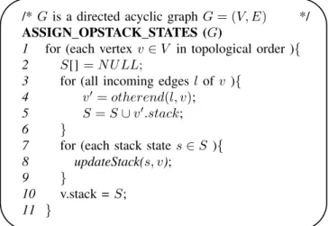
The algorithmASSIGN OPSTACK STATESin fig. 1
iden-tifies all possible control flow paths by visiting vertices of
✬
✫
✩
✪
/*Gis a directed acyclic graphG= (V, E) */
ASSIGN OPSTACK STATES (G)
1 for (each vertex v∈V in topological order ){ 2 S[]=N U LL;
3 for (all incoming edgesl of v ){
4 v′ =otherend(l, v);
5 S=S∪v′.stack;
6 }
7 for (each stack states∈S ){
8 updateStack(s, v);
9 }
10 v.stack =S;
11 }
Fig. 1. Algorithm for assigning stack states to vertices in a DAG
theDAGin topological order. This order ensures that all the predecessors of a vertexv are visited beforev itself.
The algorithm calculates a list of all possible operand stack states for the current vertexv (fig. 1: lines 2-6) by iterating all the predecessors of the vertex v and building the set of stack statesSas a disjunct union of all predecessors operand stack lists.
All stack states of the listS are updated by pop or push operations corresponding to the byte code instruction of the vertexv (fig. 1: lines 7-9).
After execution of the algorithm a list of all possible operand stack states is assigned to each vertex of theDAG.
Stack Stack states operation
-
-push a; a
push b; b
- a | b
push c; a, c | b, c
push d; a, d | b, d
- a, c | a, d | b, c | b, d ♥
v0 ✡ ✡ ✢ ❏❏
❄
♥
v1
❏❏❫ ♥
v2 ✡ ✡ ✢
♥
v3 ✡ ✡ ✢ ❏❏
❄
♥
v4
❏❏❫ ♥
v5 ✡ ✡ ✢
♥
v6
Fig. 2. CFG with operand stack states computed by the algorithm.
Theorem 3.1: (Operand Stack Algorithm) Given a di-rected acyclic graph G = (V, E), after the algorithm AS-SIGN OPSTACK STATESin fig. 1 visits a vertexv∈V, the property variable stack of v contains a list of all possible operand stack states in the vertexv.
Proof:By induction on the depth of a vertexv∈V and paths from theST ART vertex tov.
Bytecode Stack size List of variable List of variables types on the stack 0 iload_1; 1 I a
1 iload_2; 2 I,I a, b
2 if_icmple 7; 0 -
-5 iload_1; 1 I a
6 goto 4; 1 I a
9 iload_2; 1 I b
10 iconst_2; 2 I,I a, 2 | b, 2
11 invokestatic 16; 0 - -♥
v0
❄
♥
v1
❄
♥
v2
❄
♥
v5
❄ ✑ ✑
◗◗s
♥
v6 ◗◗
✑ ✑ ✰
♥
v9
❄
♥
v10
❄
♥
v11
Fig. 3. CFG, corresponding bytecode and the operand stack representation.
Induction Step: The list of all possible operand stack states
S for the vertex v with d > 0 is calculated by updating
all elements of the list S = {∀s ∈ S|update(s)} (lines
7-9). The list S is a set of all operand stack states of all immediate predecessors v0...vn of v with the depth d−1, so Sn
i=0vi.stack (lines 3-5). By induction hypothesis, each
path section from the ST ART to vi must be visited and
all operand stack states are assigned to the property variable
vi.stack.
All successorsv0...vn ofv must have a depth greater than
d, because the graph is a DAG. So the theorem holds for allv∈V with depthd >0.
Fig. 2 illustrates how the algorithm operates on the ex-ample CFG. The vertices in this exex-ample are labeled in topological order. The following control paths exist:
• p1={..., v0, v1, v3, v4, v6, ...}
• p2={..., v0, v1, v3, v5, v6, ...}
• p3={..., v0, v2, v3, v4, v6, ...}
• p4={..., v0, v2, v3, v5, v6, ...}
In path p1 the vertex v1 pushes the variable a and the vertexv4 pushes the variablec onto the stack. The operand stack states can be assigned to each vertex of path p1 as follows:p1={..., v0(−), v1(a), v3(a), v4(a, c), v6(a, c), ...}. According to these steps, the stack states in all paths can be calculated and assigned to the vertices in theDAG. But this procedure is not efficiently in terms of runtime complexity. To calculate all possible stack states in each vertex of aDAG
it is not necessary to traverse each control path separately. Instead our algorithm calculates the stack states step by step for all paths by visiting the vertices of aDAGin topological order.
Generally, the runtime complexity of a topological search
algorithm for the given directed acyclic graph G with n
vertices andm arcs can be found in O(n+m)(see [9] or [10]). The memory allocation complexity to store all possible operand stack combinations in our algorithm grows exponen-tially. As you can see from the example in fig. 2 the number
of combinations N depends on the number of sequential
branches in the DAG and equals the multiplication of the
number of branches in each branch. In this case:
N = 2×2 = 4 (1) So the complexity of the memory allocation can be calculated as O(nn
). To solve this problem a pragmatic approach
is used in our implementation. We define the maximum number of combinations which have to be calculated by the algorithm to limit the memory allocation. The number of maximum combinations is variable and can be redefined for each operand stack.
The algorithm ASSIGN OPSTACK STATES in fig. 1 can
be easily adapted to calculate the stack depth (used for size based analysis) and the list of variable types (used for type based analysis) in each node. Instead of the operand stack state combinations, a single value is stored in the property variablestackof each vertex. In this case, both the runtime
O(n +m) and the memory allocation O(n) have linear
complexity. An example of the operand stack representation is illustrated in the fig. 3.
B. Size based operand stack analysis
A size based analysis can be achieved by simply altering
the algorithmASSIGN OPSTACK STATESin fig. 1 to
calcu-late the operand stack depth value and store it in the property variable for each vertex in the corresponding CFG. By trivial comparison of the operand stack depth values assigned to the CFG’s vertices, the following types of inconsistencies can be determined:
• Stack over or underflow: The max operand stack size is calculated as the algorithm visits the vertices of the corresponding CFG in topological order. By comparing the calculated max size with the max stack size, stored in the class file, over- or underflow stack errors can be determined. The overflow verification is generally available in the JVM as specified in [2, The JavaR Virtual Machine Specification]. Our approach
also allows to determine the bytecode addresses of the instructions which cause the stack overflow.
The stack size of each end vertex (e.g. return byte in-struction) in the CFG is verified. Herewith is determined if any objects remain on the stack. By the reference to the bytecode instructions of the remained objects a warning is generated about possibly unused bytecode instructions (instructions which push these objects onto the stack).
In fig. 4 one of the three instructions, that pushes an integer value on the stack is obsolete. After the last instruction, the stack should be empty but in the example one unused integer value is left on the stack.
Bytecode Stack size
0 iload_1; 1
1 iload_2; 2
3 iconst_1; 3
4 iadd; 2
5 ireturn; 1 ♥
v0
❄
♥
v2
❄
♥
v3
❄
♥
v4
❄
♥
v5
Fig. 4. Unused objects left on stack
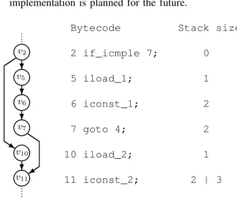
• Asymmetrical operand stack sizes: An error in one branch of the CFG could lead to asymmetrical operand stack sizes on the incoming edges of a vertex as illustrated in fig. 5. A simple backtrace algorithm to find unused instructions, is applied in our implementation. A more complex analysis algorithm and a backtrace implementation is planned for the future.
Bytecode Stack size
2 if_icmple 7; 0
5 iload_1; 1
6 iconst_1; 2
7 goto 4; 2
10 iload_2; 1
11 iconst_2; 2 | 3 ♥
v2
❄
♥
v5
❄ ✑ ✑
◗ ◗ s
♥
v6
❄
♥
v7 ◗◗
✑ ✑ ✰
♥
v10
❄
♥
v11
Fig. 5. Asymmetrical operand stack size inconsistency
The runtime complexity for this analysis is in O(n+m)
and the memory allocation complexity is inO(n), wheren
is the number of vertices andmnumber of arcs in the CFG.
C. Type based operand stack analysis
According to the JavaR Virtual Machine Specification
[2] the JVM supports the operand stack type verification in general. Gerwin Klein and Tobias Nipkow formalize and describe algorithms for an iterative data flow analysis that statically predicts the types of values on the operand stack
and in the register set [16], [14], [15] as mentioned in section II. In this section we present a graph-theoretical approach in addition to the well known verification techniques.
A type based analysis is realized by adaptation of the
algorithmASSIGN OPSTACK STATESin fig. 1 to calculate
a list of variable types on the stack and store it in the property variable for each vertex in the corresponding CFG. By comparison of the values assigned to the CFG’s vertices the following types of inconsistencies can be determined:
• Expected type: To ensure proper code execution at runtime, all operands on the stack have to be type correct in terms of what operand type the bytecode instruction expects. For example anistoreinstruction can not handle afloatoperand. Another example, as visualized in fig. 6 aniaddinstruction can not operate onintegeranddoubleoperands on the stack.
Bytecode Stack size
0 iload_1; 1
1 dload_2; 2
2 iadd; ERROR ♥
v0
❄
♥
v1
❄
♥
v2
Fig. 6. Wrong type for instruction
• Asymmetrical type lists:The types of operands on a stack can differ on the incoming edges of a vertex. The backtrace algorithm allows to reference the bytecode instructions which pushed operands with different types onto the stack.
The runtime complexity for this analysis is inO(n+m)
and the memory allocation complexity is inO(n), wheren
is the number of vertices andmnumber of arcs in the CFG.
D. Content based operand stack analysis
The algorithmASSIGN OPSTACK STATES in fig. 1
cal-culates a list of variables on the stack for each bytecode instruction and stores it in the property variable of the vertex in the corresponding CFG. In a certain vertex several variable combinations on the stack are possible.
This analysis allows to figure out unnecessary branches in the bytecode. The bytecode example in fig. 7 contains an if-branch. The bytecode instructions (offset 5 and 9) in both branches push the same variable b onto the stack. A backtrace algorithm prints the bytecode addresses of instructions which lead to the duplicated operand stack states. This kind of analysis is related to compiler optimization techniques, but in our approach the operand stack analysis is used to localize unused instructions. Our approach is partially comparable to the method of Lim and Han described in their paper [18, Analyzing Stack Flows to Compare Java Programs]. Although the goal of their paper is to identify clones of Java programs, the approach is absolutely different. The runtime complexity for this analysis is inO(n+m), wherenis the number of vertices andmnumber of arcs in the CFG. The memory allocation complexity is inO(nn
Bytecode List of variables on the stack
2 if_icmple 7;
-5 iload_2; b
6 goto 4;
9 iload_2; b
10 iconst_2; b, 2 | b, 2 ♥
v2
❄
♥
v5
❄ ✑ ✑
◗ ◗ s
♥
v6 ◗◗
✑ ✑ ✰
♥
v9
❄
♥
v10
Fig. 7. Operand Stack with the same content in two branches
E. Loop based operand stack analysis
This section extends the analysis algorithms to arbitrary control flow graphs that can contain cycles. The algorithm fig. 1 in section III-A only works for acyclic paths, which correspond to back edge free paths. The main idea of the loop based analysis is that the operand stack states before entering and after leaving a loop have to be equal. Otherwise, each iteration of the loop would push objects onto the stack or pop them from the stack and the state of the stack would be undefined.
A depth-first search algorithm identifies a set of back edges
B ⊂ E in a graph G = (V, E), that contains cycles. The
graphGis transformed into a directed acyclic graph (DAG) by removing the back edgesD= (V, E′), whereE′ =E\B. Each back edgeb∈B lies on a loop.
Theorem 3.2: (Loop Analysis Algorithm) The operand
stack of a method represented by a control flow graph G
that contains cycles is consistent if:
1) Size based analysis (section III-B) and type based analysis (section III-C) have been performed without any error on the directed acyclic graphD transformed from the graphG.
2) and for each back edgeb∈Bwith the start vertexvs∈
V and the end vertex ve∈V: the operand stack state assigned to the start vertexvs and the states assigned to the start verticesv0, ...vn of all incoming edges of the end vertexve are equal in size and type.
Proof: The point 1 of the theorem does not need to be proofed, because in case of any errors the stack is inconsistent. The point 2 can be proofed by the contradiction of the operand stack states.
♥
v0
✠ ..
.
♥
vn
❅ ❅ ■
♥
vs
❅❅❘b
♥
ve
✠ ✲
Fig. 8. Loop based analysis
Let us consider the directed acyclic graphDproduced by removing the back edges and the set of back edges B. For each b∈B holds:
• Each back edgeb∈B lies on one loop.
• There are possibly several forward paths ve → ... →
vs→ve in the loop.
Each forward path must have the same operand stack state in the last vertex, because all paths are acyclic and they pass the back edgeb. All acyclic paths have already been verified by the point 1 of the theorem.
The back edge b is a single back edge of the vertex vs, because all other edges are outside the loop and must belong to theDAG. So all states of other incoming edges have been already verified by the point 1 of the theorem.
If the state of the vertexvewould not be equal to the states of verticesv0...vn then the stack would be inconsistent.
The following algorithm for the loop based analysis is derived from the theorem 3.2. The algorithm executes the
✬
✫
✩
✪
/*D= (V, E′)is a directed acyclic graph. B is a */ /* set of back edges,B*E′. The back edge b∈B, */
/*b={vs, ve}, where vs, ve∈V. */
LOOP ANALYSIS (D, B)
1 for (each back edgeb∈B ){
2 for (all incoming edgesl of ve){
3 v=otherend(l, ve);
4 if(v.stack6=vs.stack){
5 printERROR;
6 } } }
Fig. 9. Loop based analysis algorithm
operand stack comparison for all back edgesb∈Bidentified in the previous step of the analysis. The runtime complexity for this analysis is inO(n+m)wheren is the number of vertices andmnumber of arcs in the CFG.
Bytecode Stack size
0 iload_1; 1
1 iload_2; 2
2 iconst_1; 3
3 iadd; 1
4 goto -4; 1 ♥
v0
❄
♥
v1
❄ ✑✑✸
◗◗
♥
v2
❄
♥
v3
❄
♥
v4
Fig. 10. Loop based analysis example
Fig. 10 shows an example where the loop based analysis tracks down the error in the loop in which a newinteger
stays on the stack after each loop execution.
IV. VISUALIZATION OF THEOPERANDSTACK
The simplest way to visualize the operand stack is to cal-culate the state of the operand stack in each instruction of a method and display the complete list of instructions with cor-responding states. The calculation of the operand stack states
is performed by the algorithm ASSIGN OPSTACK STATES
operand stack content more comprehensible we have defined a grammar (see appendix A) which includes variable types and names, logical combination and arithmetical operations and developed an algorithm to transform the control flow graph of a method to a tree representation.
✬
✫
✩
✪
/*Gis a control flow graph,G= (V, E). */
TRANSFORM GRAPH (G)
1 Gb=createBasicBlockGraph(G);
2 removeBackEdges(Gb);
3 T = createTree(); /*T is an empty tree. */
4 for (all start basic blocksB∈Vb)
5 CREAT E T REE(B, T);
6 };
CREATE TREE (B,T)
1 add a new tree noden forB toT;
2 for ( all vertices v∈B ){
3 addv as child ofn to the treeT;
4 }
5 for (all outgoing argsl of B ){
6 CREAT E T REE(otherend(l, B), T);
7 }
Fig. 11. Transformation algorithm for the operand stack representation
The algorithm TRANSFORM GRAPH in fig. 11 creates
a basic block graph Gb for the given control flow graph G (line 1), removes the back edges in Gb (line 2) and starts a Depth First Searchfrom each start basic block B, where
indegree(B) = 0(line 4). For each basic blockBa new tree node nis created (Routine CREATE TREE: line 1) and all vertices of a basic blockB(each vertex represents a bytecode instruction) are added as children ofBto the treeT (Routine
CREATE TREE: lines 2-4). The bytecode instruction treeT
is used to represent the operand stack structure in a view.
Fig. 12. Operand stack representation
An example representation of a Java bytecode is shown in fig. 12.
V. DYNAMICOPERANDSTACKVISUALIZATION AND VERIFICATION
The static representation of the operand stack can be extended by the dynamic visualization. The dynamic rep-resentation can only be created during the execution of the program, usually during a debugging session. If the operand stack state at the certain point of the execution has to be analyzed, the task to represent the operand stack is trivial. For this purpose the values on the stack just have to be read from the execution environment, if the runtime environment supports the access to the operand stack. Unfortunately, the JVM-implementation, based on the JVM-specification [2], does not provide any access to the operand stack via debug-ging interface [3]. Nevertheless, it is possible to visualize the operand stack values by using the local variables.
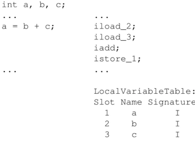
Let us consider the linea = b + c;from the following Java source code example and the corresponding bytecode:
int a, b, c;
... ... a = b + c; iload_2;
iload_3; iadd; istore_1; ... ...
LocalVariableTable: Slot Name Signature
1 a I 2 b I 3 c I
Fig. 13. Source code example and the corresponding bytecode
The iadd instruction adds two int values together.
It requires that the int values to be added be the top
two values of the operand stack, pushed there by previous instructionsiload_2andiload_3. Since the instructions
iload_2andiload_3are linked to the variablesbandc, their values can be obtained via debugging interface. Both
of the int values are popped from the operand stack by
executing theiaddinstruction and their sum is pushed back onto the operand stack. For visualization purposes the result can be calculated or represented as an arithmetic chain.
Bytecode Stack ...
iload_2; b = 3
iload_3; b = 3, c = 1 iadd; b + c = 4 istore_1;
...
Fig. 14. Dynamic operand stack visualization
a part of the operand stack history is missing. The operand stack state in this case can not be represented. The next sub-sections describe how to record and verify the operand stack history efficiently.
A. Operand Stack Visualization of Loops
We assume that the bytecode is executed step by step, and the state of the operand stack is logged for each instruction. Let be V the set of bytecode instructions of a method and
R the set of the operand stack records. In order to keep the memory allocation linear, the number of records have to be less than or equal to the number of instructions.
|R| ≤ |V| (2)
Let be V′ ⊆V the set of loop instructions. So the number of the operand stack records can be calculated as
|R|=n× |V′|, (3) wherenthe number of the loop iterations. As the number of iterations cannot be predicted, the length of the stack history may be very large.
Our proposed solution is to store the state of the stack only once per instruction to satisfy the condition of the equation 2. An additional counter stores information how often an instruction has been executed. According to the theorem 3.2
Bytecode Iterations Stack Stack size
0: iload_1 10 1 a 1: iload_2 10 2 a, b 2: if_icmpge 11 10 0 -5: iinc 1, 1 9 0 -8: goto 0 9 0 -11: return 1 0
-Fig. 15. Example of the operand stack representation with a loop.
(subsection III-E), the state of the operand stack in each iteration must be the same with the prerequisite that the bytecode is free of errors. To visualize potential errors the stored operand stack state is compared with the current state in the next iteration. If the states are not equal in terms of size and content, an error is reported. This makes it possible
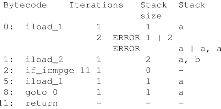
Bytecode Iterations Stack Stack size
0: iload_1 1 1 a 2 ERROR 1 | 2
ERROR a | a, a 1: iload_2 1 2 a, b 2: if_icmpge 11 1 0 -5: iload_1 1 1 a 8: goto 0 1 1 a 11: return - -
-Fig. 16. Example of the operand stack representation with a loop.
to determine which iteration of the loop has caused the error. In fig. 16 an example of an error is presented. After the first iteration the variable a, pushed by the instruction
5: iload_1, remain on the stack. The comparison of
the states during the second iteration detects a difference. Such an error can of course be found with the static loop analysis. However, if the bytecode is generated at runtime, such errors can be only found by dynamic stack analysis.
B. Breakpoint Handling
For debugging purposes, the program is not always exe-cuted step by step. The developer sets a breakpoint, at which the program execution will be stopped. If the runtime envi-ronment, such as JVM [2], [3], allows only limited access to the operand stack, it is not possible to represent the complete content of the operand stack. Our proposed solution is to combine the static representation of the operand stack with the available and accessible operands. The reconstruction algorithm is represented in fig. 17. The input of the algorithm
✬
✫
✩
✪
/*Gis a control flow graph,G= (V, E). */
DYN OPSTACK REPRESENTATION (G,vs)
1 removeBackEdges(G);
2 V′ = backwardsDF S(v); /*V′∈V */
3 G′ = createSubgraph(G, V′);
4 ASSIGN OP ST ACK ST AT ES(G′);
5 DY N OP ST ACK(G′, v);
DYN OPSTACK (G,v)
1 if ( dynamic opstack state ofv not available ){
2 return;
3 }
4 replace static by dynamic values;
5 for (all incoming argsl of v ){ 6 v′ = otherend(l, v);
7 DY N OP ST ACK(G, v′);
8 }
Fig. 17. Algorithm for the dynamic operand stack representation
DYN OPSTACK REPRESENTATIONis a control flow graph
Grepresenting a method and a vertex vs ∈V representing the instruction, where the execution of the code has been stopped.
The algorithm removes the back edges in the graphG(line 1) to create aDAG. The routine backwardsDFS (line 2) is a backward Depth First Searchwhich returns the set of all vertices V′ (bytecode instructions) reachable via backward
paths from the vertex v. In the line 3 a subgraph of G
containing the vertices fromV′is created. The algorithm
AS-SIGN OPSTACK STATES(fig. 1 from the subsection III-A) assigns the static operand stack states to all vertices from the setV′. The routine DYN OPSTACK starts the replacement of statically calculated operand stack states by the available dynamic values as described at the beginning of the section V. The routine is called recursively and it stops as soon as the dynamic value of the operand stack is not available or can not be calculated.
Let us consider the Java source code example in fig. 18. The corresponding bytecode is presented in fig. 19. The bytecode contains three operands representing the variables
a,b andc. Lets us assume that a breakpoint is set in line
int c = a < b ? a + b : b - a; return c;
Fig. 18. Source code example.
and we are able to read the current values of the operands
a,bandcvia Java debugging interface.
int c = a < b ? 0 iload_0; /* a */ a + b : 1 iload_1; /* b */
2 if_icmpge 9;
5 iload_0; /* a */ 6 iload_1; /* b */ 7 iadd;
8 goto 6;
b - a; 11 iload_1; /* b */ 12 iload_0; /* a */ 13 isub;
14 istore_2; /* c */ return c; 15 iload_2; /* c */
16 ireturn;
Fig. 19. Bytecode to source code example in fig. 18.
To visualize the operand stack the algorithm
DYN OPSTACK REPRESENTATION in fig. 17 executes
following steps. The input is a Graph G containing all
instructions of the bytecode V and the instruction vs with
the bytecode address 15 at which the program has been
stopped. The line 1 is ignored because for simplicity our
example does not contain any loops. The backwardsDFS
procedure collects backwards all from vs reachable
instructions and stores them in V′. The set V′ includes all instructions ofV accept the last one with bytecode address
16. Based onV′ a subgraphG′ is generated. The algorithm
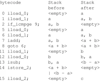
ASSIGN OPSTACK STATESfrom the subsection III-A, fig. 1, will assign statically the following operand stack states (fig. 20). The column Stack before represents the state of
Bytecode Stack Stack before after 0 iload_0; <empty> a 1 iload_1; a a, b 2 if_icmpge 9; a, b <empty> 5 iload_0; <empty> a
6 iload_1; a a, b 7 iadd; a, b <a + b> 8 goto 6; <a + b> <a + b> 11 iload_1; <empty> b
12 iload_0; b b, a 13 isub; b, a <b - a> 14 istore_2; <a + b> <empty>
| <b - a> 15 iload_2; <empty> c
Fig. 20. Static operand stack visualization of the bytecode in fig. 19.
the operand stack before the bytecode instruction has been executed and the columnStack afterthe state of the operand stack after the execution of the bytecode instruction. The recursive routine DYN OPSTACK starts from the vertex vs
representing the bytecode instruction 15 iload_2 and
visualize following values. For example the obtained values of the operands a, b and c are: a = 3, b = 2 and c = 5. The dynamic visualization of the operand stack is presented in fig. 21. The value of the operandc is obtained from the
Bytecode Stack Stack before after 0 iload_0; <empty> a=3 1 iload_1; a=3 a=3, b=2 2 if_icmpge 9; a=3, b=2 <empty> 5 iload_0; <empty> a=3 6 iload_1; a=3 a=3, b=2 7 iadd; a=3, b=2 <a + b>=5 8 goto 6; 5 5
11 iload_1; - -12 iload_0; - -13 isub; -
-14 istore_2; 5 <empty> 15 iload_2; <empty> c=5
Fig. 21. Dynamic operand stack visualization of the bytecode in fig. 19.
execution environment. So the stack of the instruction with the address 15 and 14 is visualized. To visualize the stack states in the if branches the arithmetic operation has to be interpreted and two equations have to be solved.
a+b=c b−a=c
3 + 2 = 5 true 3−2 = 1 f alse
After solving the equations we can exclude one branch and replace the mathematical operations by the calculated values as presented in fig. 21.
If not all operand stack states can be dynamically visual-ized the mix of the static and dynamically calculated states can be represented.
VI. EXPERIMENTAL RESULTS
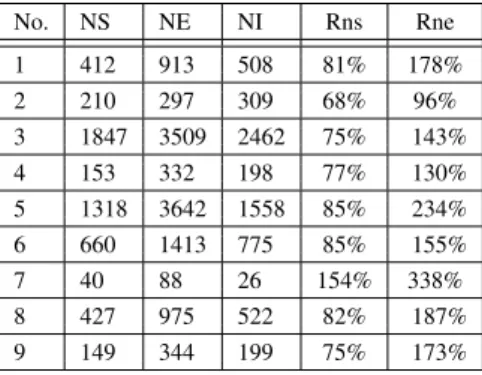
As stated in section III-A the more combinations of se-quential branches are contained in the bytecode of a method, the more memory needs to be allocated. In practice, excessive memory allocation happens very rarely. We analyzed over 500 methods from different Java classes of the Standard Java Library with the implementation based on the Dr. Garbage tools [8], [7]. The most representative methods are listed in the table I which have been selected by the following criteria:
• methods with a large number of bytecode instructions
• methods that contain a large number ofifor switch
instructions
• methods with a large stack size
• methods that hold a decent amount of stacks
The columnNSin the table I represents the number of stack objects generated for a method. Each stack object is assigned to a bytecode instruction and represents the current state of the stack in this instruction. The memory consumption would stay linear if the number of stack objectsNSis less or equal the number of bytecode instructionsNI in a method.
TABLE I
EXPERIMENTALRESULTS: MS -MAX STACK SIZE, MC -MAX NUMBER OF STACK COMBINATIONS, NS -NUMBER OF STACKS, NE -TOTAL NUMBER OF STACK ENTRIES, NI -NUMBER OF BYTECODE INSTRUCTIONS, IF/S -NUMBER OF IF/SWITCH INSTRUCTIONS
No. Library Package Class Name Method Name MS MC NS NE NI IF/S
01 classes.jar sun.awt.geom Curve compareTo() 31 1 412 913 508 25/0
02 classes.jar com.sun.imageio.metadata XmlChars isCompatibilityChar() 2 2 210 297 309 85/1
03 j3dcore.jar javax.media.j3d Font3D triangulateGlyphs() 6 2 1847 3509 2462 84/0
04 classes.jar java.util SimpleTimeZone makeRulesCompatible() 4 1 153 332 198 8/4
05 vecmath.jar javax.vecmath Matrix3d compute svd() 10 1 153 332 1558 19/0
06 j3dcore.jar javax.media.j3d Alpha value() 5 1 660 1413 775 39/0
07 classes.jar sun.tools.tree BinaryExpression costInline() 5 4 40 88 26 2/0
08 classes.jar sun.io ByteToCharUTF8 convert() 7 1 427 975 522 21/0
09 classes.jar javax.print ServiceUI printDialog() 10 1 149 344 199 19/0
The number of generated stacks could be less than the number of bytecode instructions in the method, because not all instructions operate with the stack or greater
if the stack combinations according the algorithm
AS-SIGN OPSTACK STATESin fig. 1, section III-A have to be calculated.
The columnNE in the table I represents the total number of stack entries calculated as defined in equation 5, where
BI the list of bytecode instructions.
N E= X
e∈BI
e.stack.size() (5)
To make the collected results relative and to show how the number of generated stacks and stack entries depend on the number of instructions we calculate for each method the relative value Rns as a ration of the number of stacksN S to the number of bytecode instructionsN I (equation 6)
Rns=
N S
N I100% (6)
and the relative value Rne as a ration of the number o
stack entriesN Eto the number of bytecode instructionsN I
(equation 7).
Rne=
N S
N I100% (7)
The calculated values are summarized in the table II and presented in the chart in fig. 22. The ration of the number
TABLE II
EXPERIMENTALRESULTS:RELATIVE VALUES
No. NS NE NI Rns Rne
1 412 913 508 81% 178%
2 210 297 309 68% 96%
3 1847 3509 2462 75% 143%
4 153 332 198 77% 130%
5 1318 3642 1558 85% 234%
6 660 1413 775 85% 155%
7 40 88 26 154% 338%
8 427 975 522 82% 187%
9 149 344 199 75% 173%
of generated stacks to the number of bytecode instructions
Rns is under 100% for all methods except the method
BinaryExpression.costInline(). According the table I the max number of stack combinations for this method is 4 and this
is the reason why theRns value is higher. Nevertheless the value of 154% is acceptable. The memory consumption is still linear, becauseO(2n)⇒O(n), wherenthe number of bytecode instructions.
m1 m2 m3 m4 m5 m6 m7 m8 m9 0
100 200 300
Rns Rni
Fig. 22. Ration of the number of stacksN S to the number of bytecode instructionsN I
The ration of the number of generated stack entries to the number of bytecode instructions Rne is much more higher than theRns value, because stack objects may contain more than one entry. The number of stack entriesN Edepends on the max stack size of a method. Although theRnsvalue for the methodBinaryExpression.costInline()is about 350% the memory allocation stays linear. In our implementation the stack entries are reused and only the references are stored in stack objects. In this way the number of allocated stack entries is always equal or less the number of stack objects. The fig. 23 presents an example of the stack allocation.
S1 SE1 S2 SE1,SE2 S3 SE1,SE2,SE3 S4 SE1,SE2 S5 SE1
Fig. 23. Stack allocation
the example above would get the value nine, according the equation 5.
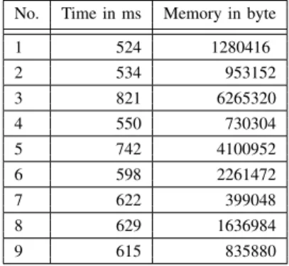
N E=S1.size+...+S5.size= 1+2+2+3+2+1 = 9 (8) The absolute runtime time and memory allocation values of the implemented algorithms are presented in table III.
TABLE III
EXPERIMENTALRESULTS:TIME AND MEMORY ANALYSIS
No. Time in ms Memory in byte
1 524 1280416
2 534 953152
3 821 6265320
4 550 730304
5 742 4100952
6 598 2261472
7 622 399048
8 629 1636984
9 615 835880
The experimental results have shown that despite a number of conditional branch operators or stack entries along with method instructions, the amount of stack combinations stay in limit. The run time and memory allocation measurements shows as well that the implemented algorithms are suitable for usage in developer environments.
VII. CONCLUSION
This paper describes new algorithms for operand stack analysis and visualization based on graph theoretical meth-ods. Although the algorithms partially execute trivial operand stack verifications, they can be obtained as a supplement to the well known algorithms. The operand stack visualization algorithms presented in this paper are the first that can represent the operand stack in such a comprehensive way.
Experimental results showed that the performance and memory consumption do never deviate from linearity, al-though the theoretical memory consumption has exponential complexity. It is obviously possible with the synthetically generated code to reach the limits, but such code constructs do not occur in practice. We are convinced that a lot of new tools can be designed and implemented based on these algorithms and results
APPENDIXA
OPERANDSTACKCONTENTGRAMMAR
<Stack> ::= <StackEntry>{"," <StackEntry>}{"|" <Stack>} <StackEntry> ::= <type> <value>
<type> ::= "B" | "C" | "D" | "F" | "I" | "J" | "S" | "Z" | "L" | <array type>
<array type> ::= "[" { "[" } <type>
<value> ::= <variable name> | <constant> | <array name> | <math operation>
<variable name> ::= <char>{<char>}
<char>::= any one of the 128 ASCII characters, but not any of special characters [, ], (, ), \, /, ;, ... or the space character
<constant> ::= 0 | 1 | 2 | 3 | 4 | 5 | 6 | 7 | 8 | 9 | <float_constant> {<constant>}
<array name> ::= <variable name> [ <numeric> | <variable name> ]
<float_constant> ::= <constant> "." <constant>
<math operation> ::="("<value> <operation> <value>")" <operation> ::= "+" | "-" | "*" | "/" | "%" | "ˆ" | "|"
| "<<" | ">>"
ACKNOWLEDGMENT
The authors would like to thank the Dr. Garbage Project Community for supporting the implementation of proposed algorithms and tools [7].
REFERENCES
[1] Sergej Alekseev, Andreas Karoly, Duc Thanh Nguyen and Sebastian Reschke, Graph Theoretical Algorithms For JVM Operand Stack Visu-alization And Bytecode Verification, Lecture Notes in Engineering and Computer Science: Proceedings of The World Congress on Engineering and Computer Science 2013, WCECS 2013, 23-25 October, 2013, San Francisco, USA, pp12-17
[2] Tim Lindholm, Frank Yellin, Gilad Bracha and Alex Buckley,
The JavaR Virtual Machine Specification, Java SE 7 ed., 2013, http://docs.oracle.com/javase/specs/jvms/se7/html/
[3] Oracle and/or its affiliates, The JavaR Platform
Debugger Architecture (JPDA), Java SE 7 ed., 2013, http://docs.oracle.com/javase/7/docs/technotes/guides/jpda/
[4] Bruce Ian Mills, Theoretical Introduction to Programming, Springer 2006, ISBN 978-1-84628-263-8
[5] Adobe Systems,PostScript language reference. 3.Edition , Addison-Wesley 1999, ISBN 0-201-37922-8
[6] Leo Brodie,Starting FORTH: an introduction to the FORTH language and operating system for beginners and professionals, Prentice-Hall 1987, ISBN 0-201-37922-8
[7] Sergej Alekseev, Peter Palaga and Sebastian Reschke,The Dr. Garbage Tools Project, 2013, http://www.drgarbage.com
[8] Sergej Alekseev, Victor Dhanraj, Sebastian Reschke, and Peter Palaga, Tools for Control Flow Analysis of Java Code, Proceedings of the 16th IASTED International Conference on Software Engineering and Applications, 2012, http://www.actapress.com/PaperInfo.aspx?paperId=454811
[9] G¨unther Stiege,Graphen und Graphalgorithmen, Shaker;Auflage: 1, 2006, ISBN 3832251138
[10] Donald E. Knuth,The Art of Computer Programming, Addison Wesley, 1997, ISBN 0201896834
[11] Xavier Leroy, Java bytecode verification: an overview, Computer Aided Verification, CAV 2001, Vol. 2102 of Lecture Notes in Computer Science, pages 265-285. Springer, 2001.
[12] Xavier Leroy,Java bytecode verification: algorithms and formaliza-tions, Journal of Automated Reasoning, Vol. 30 Issue 3-4, Pages 235 - 269, 2003, http://gallium.inria.fr/ xleroy/publi/bytecode-verification-JAR.pdf
[13] Stephen N. Freund, John C. Mitchell, A Type System for the Java Bytecode Language and Verifier, Journal of Auto-mated Reasoning, Vol. 30 Issue 3-4, Pages 271 - 321, 2003, http://theory.stanford.edu/people/jcm/papers/03-jar.pdf
[14] Gerwin Klein, Tobias Nipkow,Verified lightweight bytecode verifica-tion, Concurrency and Computation: Practice and Experience, Vol. 13, Pages 1133-1151, 2001
[15] Gerwin Klein, Tobias Nipkow, Verified bytecode verifiers, Journal Theoretical Computer Science, Vol. 298, Issue 3, Pages 583 - 626, 2003, http://tumb1.biblio.tu-muenchen.de/publ/diss/in/2003/klein.pdf [16] Gerwin Klein, Martin Wildmoser,Verified Bytecode Subroutines,
Jour-nal of Automated Reasoning, Vol. 30 Issue 3-4, Pages 363 - 398, 2003, http://www.cse.unsw.edu.au/ kleing/papers/KleinW-TPHOLS03.pdf [17] Eva Rose,Lightweight Bytecode Verification, Journal of Automated
Reasoning, Vol. 31, Issue 3-4, Pages 303-334, 2003
[18] Hyun-il Lim, Taisook Han,Analyzing Stack Flows to Compare Java Programs, EICE Transactions 95-D(2), Pages 565-576, 2012 [19] Alessandro Coglio,Simple verification technique for complex Java
bytecode subroutine, In Proc. 4th ECOOP Workshop on Formal Tech-niques for Java-like Programs, 2002
[20] Robert St¨ark, Joachim Schmid, and Egon B¨orger,Java and the Java Virtual Machine - Definition, Verification, Validation, Springer, 2001. [21] R. Stata and M. Abadi,A type system for Java bytecode subroutines, In
Proc. 25th ACM Symp. Principles of Programming Languages, Pages 149–161. ACM Press, 1998.