www.nonlin-processes-geophys.net/14/789/2007/ © Author(s) 2007. This work is licensed
under a Creative Commons License.
in Geophysics
Modeling pairwise dependencies in precipitation intensities
M. Vrac1, P. Naveau1, and P. Drobinski2
1Laboratoire des Sciences du Climat et de l’Environnement, IPSL-CNRS, Gif-sur-Yvette, France 2Service d’A´eronomie, IPSL-CNRS, Universit´e Pierre et Marie Curie, Paris, France
Received: 29 August 2007 – Revised: 19 November 2007 – Accepted: 19 November 2007 – Published: 5 December 2007
Abstract. In statistics, extreme events are classically de-fined as maxima over a block length (e.g. annual maxima of daily precipitation) or as exceedances above a given large threshold. These definitions allow the hydrologist and the flood planner to apply the univariate Extreme Value Theory (EVT) to their time series of interest. But these strategies have two main drawbacks. Firstly, working with maxima or exceedances implies that a lot of observations (those below the chosen threshold or the maximum) are completely disre-garded. Secondly, this univariate modeling does not take into account the spatial dependence. Nearby weather stations are considered independent, although their recordings can show otherwise.
To start addressing these two issues, we propose a new statistical bivariate model that takes advantages of the re-cent advances in multivariate EVT. Our model can be viewed as an extension of the non-homogeneous univariate mixture. The two strong points of this latter model are its capacity at modeling the entire range of precipitation (and not only the largest values) and the absence of an arbitrarily fixed large threshold to define exceedances. Here, we adapt this mixture and broaden it to the joint modeling of bivariate precipita-tion recordings. The performance and flexibility of this new model are illustrated on simulated and real precipitation data.
1 Introduction
There exists a wide range of distribution families to statisti-cally model rainfall intensities. For example, Katz (1977), Vrac et al. (2007), and Wilks (2006) argued that most of the precipitation variability can be approximated by Gamma dis-tributions. However, it is also well known (e.g. Katz et al., 2002) that the tail of the Gamma distribution can be too light
Correspondence to:M. Vrac ([email protected])
to capture heavy rainfall intensities. This leads to the un-derestimation of return levels and others quantities linked to high percentiles of precipitation amounts. Consequently, the societal and economical impacts associated with heavy rains (e.g., floods) can be miscalculated. To solve this issue, an increasingly popular approach in hydrology (e.g. Katz et al., 2002) is to disregard small precipitation values and to focus only on the largest rainfall amounts. The advantage of this strategy is that an elegant mathematical framework called Ex-treme Value theory(EVT) developed in 1928 by Fisher and Tippett (1928) and regularly updated during the last decades (e.g. Resnick, 2007; De Haan and Ferreira, 2006) dictates the distribution of heavy precipitation. More specifically, EVT states that rainfall exceedances, i.e. amounts of rain greater than a given thresholdu, can be approximated by a General-ized Pareto Distribution (GPD) if the threshold and the num-ber of observations are large enough.
0 10 20 30
0
10
20
30
St Alban
Perreux
0 5 10 15 20 25
0
5
10
15
20
25
Perreux
Riorges
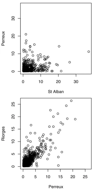
Fig. 1. The top panel shows the scatterplot between daily precip-itation data in mm/day recorded at two French stations named St Alban and Perreux which are fairly far away from each other (about 300 km). In contrast, the bottom panel displays the same type of scatterplot but between two nearby stations, Perreux and Riorges (about 10 km).
extension can be trivial for some distributions. This is not the case here because the EVT is different in the 2-D case. While univariate EVT imposes a parametric form for the margins, bivariate EVT forces the dependence structure among ex-tremes to be non-parametric and choices have to be made to deal with this problem (e.g. see Chapter 8 of Coles, 2001). In addition, modeling the transition from the bulk of the dis-tribution to the extreme values represents an additional chal-lenging task.
The paper is organized as follows. In Sect. 2 we give a brief overview of the precipitation measurements that will be used to illustrate and validate our approach. We also recall
a few basic concepts used in bivariate EVT. Section 3 is di-vided into two parts. Firstly, we treat the univariate case by recalling the basic principles of the Frigessi mixture model Frigessi et al. (2002) and by applying it to univariate precip-itation recordings. Secondly, we propose a bivariate model that combines the advantages of the Frigessi univariate mix-ture model and the principles of bivariate EVT. Section 4 fo-cuses on applications. Our approach is tested on simulated data and applied to precipitation measurements. Finally, we summarize our results and discuss some future research di-rections in Sect. 5.
2 Precipitation data
To exemplify the methodologies proposed in this paper, we will analyze rainfall measurements coming from three weather stations located near the cities of St Alban, Perreux and Riorges that belong to the French Mediterranean region. In this section we present the basics statistical properties of these observations. The daily time series cover the time pe-riod from 1 January 1994 to 31 December 2004.
coordinates, a radius and a pseudo “angle”ω(e.g. see Chap-ter 8 of Coles, 2001) defined by
ω= R2
|R|, with|R| =R1+R2. (1) The effect of transforming the vector(R1,R2)into(|R|, ω) defined by Eq. (1) will be illustrated in Sect. 4 on simulated and real precipitation data. Because the angle takes its val-ues between zero and one, one classical model is the Beta probability density function
bβ(ω)=
Ŵ(β1+β2) Ŵ(β1)Ŵ(β2)
ωβ1−1(1−ω)β2−1, (2)
withω∈[0,1]and whereŴ(.)is the Gamma function andβi
are positive reals. The Beta density offers a wide range of density shape while keeping the number of parameters under control. It also has the advantage to have well-known prop-erties.
From a theoretical point of view, it is interesting to see that the joint probability of the angle and the radius (ω,|R|) given that|R|>xfor some largexcan be written as
P(|R|> rxandω∈ [a, b])
P(|R|> x) =
P(|R|> rx)
P(|R|> x)P(ω∈ [a, b])
if 0<a<b<1 and|R|is independent ofω. In addition, if the radius is assumed to be regularly varying with index−1/ξ, i.e.,
lim
x→∞
P(|R|> rx)
P(|R|> x) =c r −1/ξ
, for some constantc >0, then it follows
lim
x→∞
P(|R|> rxandω∈ [a, b])
P(|R|> x) =cr −1/ξ
P(ω∈ [a, b]).
Hence, defining pseudo-coordinates is closely linked to the concept ofregular variationand the latter has been increas-ingly popular in multivariate EVT during the last decades, specially in time series analyses for heavy-tailed models (e.g. Resnick, 2007; De Haan and Ferreira, 2006; Beirlant et al., 2004).
3 Our statistical models
3.1 The univariate case
According to basic univariate EVT (e.g. Coles, 2001; Em-brechts et al., 1997), the probability that large rainfall amount, say the random variable R, is larger than the real r given thatR is already larger than a fixed high threshold ucan be approximated by a Generalized Pareto Distribution (GPD) tail defined as
P(R > r|R > u)=
1+ξr−u σ
−1/ξ
+
, (3)
wherea+=max(a,0)andσ >0 represents the scale param-eter. The shape parameterξ describes the GPD tail behav-ior. Ifξ is negative, the upper tail is bounded. Ifξ is zero, this corresponds to the case of an exponential distribution (all moments are finite). Ifξ is positive, the upper tail is still unbounded but higher moments eventually become infinite. These three cases are termed “bounded”, “light-tailed”, and “heavy-tailed”, respectively. The flexibility of the GPD to describe three different types of tail behavior makes it a uni-versal tool for modeling exceedances. In our case, we assume that our rainfall data are heavy-tailed, i.e.ξ is assumed to be positive. We also note that the GPD belongs to the family of regularly varying function introduced at the end of Sect. 2
A possible drawback of EVT is that the GPD only models data exceeding a given high threshold, and one can wonder how to model the remaining data (i.e. lower than the thresh-old) or equivalently how to deal with the entire range of data. To answer these questions, Frigessi et al. (2002) proposed the following mixture model
fθ(r)=cθ
h
(1−pµ,τ(r)) gγ(r)+pµ,τ(r) hσ,ξ(r)
i
, (4) wherecθis a normalizing constant,θ=(µ, τ,γ, σ, ξ ) encap-sulates the vector of unknown parameters,gγ corresponds to a light-tailed density with parametersγ, the function hσ,ξ
represents a heavy tailed Generalized Pareto (GP) density with thresholdu=0. One of the most interesting aspect of Eq. (4) is the weight functionpµ,τ(.)defined by
pµ,τ(r)=
1 2 +
1 π arctan
r−µ
τ
. (5)
Because this weight function is non-decreasing, takes val-ues in[0,1]and tends to 1 asr goes to∞, it can play the role of an unsupervised threshold selection algorithm. This transition can be interpreted as the contribution of the GPD to the overall fit. For our case study, heavy rains are repre-sented by the heavy tailed GPD densityhσ,ξ(r), while low
and medium precipitation are modeled by the light distribu-tiongγ. Concerning the weight function pµ,τ(r), our past
work (Vrac and Naveau, 2007) suggested that τ is almost equal to zero for rainfall data. This is also the case for our Mediterranean precipitation. Hence,τ is fixed to zero in the rest of this article. In other words, the weight function is set to the limit of Eq. (5) asτ tends to 0, i.e.
pµ,0(r)=
(
1 , ifµ≤r, 0 , otherwise.
This special case has the advantage of reducing the number of parameters, although, for other applications, the more gen-eral form ofpµ,τ(r)defined by Eq. (5) may be more
Histogram of Perreux
precipitation (mm/day)
Density
0 5 10 15 20
0.0
0.1
0.2
0.3
0.4
0 2 4 6 8 10 12
0
2
4
6
8
10
12
QQplot for Perreux
Modeled precipitation quantiles
Observed precipitation quantiles
Fig. 2.Top panel: Histogram of the positive precipitation measure-ments from Perreux. Dashed and solid lines correspond to a Gamma fit and a mixture (Eq. 4) fit, respectively. Bottom panel: QQplots of the positive Perreux precipitation data (in mm/day) with the two fit-ted distributions. The x-axis corresponds to the expecfit-ted quantiles and the y-axis represents the observed quantiles. The crosses and the circles correspond to the estimated Gamma and mixture quan-tiles, respectively.
While Frigessi et al. (2002) chose to parametrize the light densitygγ as a Weibull density in their fire loss application, we opt to representgγ by a Gamma density for our precipi-tation data. This choice appears to be in compliance with the past hydrological literature on precipitation modeling (e.g. Katz, 1977; Vrac et al., 2007; Wilks, 2006). The Gamma
density is defined as
gγ(r)= γγ1
2 Ŵ(γ1)r
γ1−1exp(−rγ
2), forr >0. (6) The mixture model between a light Gamma density and a heavy-tailed GPD has already been applied to downscale rainfall data over the state of Illinois (USA) (Vrac and Naveau, 2007). In this past study, weather stations were considered independent in space while the parameters of the mixture model were conditioned to large scale climatic in-formation. In this respect, the present work represents a dif-ferent direction because the pairwise spatial dependence will be directly addressed in the coming sections.
To establish the superiority of the mixture model (Eq. 4) for our data over a simple Gamma density, the histogram (top panel) and the quantile-quantile plot (QQplot) (low panel) of the positive rainfall amounts recorded at the Perreux weather station are shown in Fig. 2. In the top panel of Fig. 2, the dashed and solid lines correspond to a Gamma fit and a mixture fit, respectively. This indicates that the mixture model defined by Eq. (4) provides a reasonably good fit of the core of the rainfall distribution. Concerning the ex-tremes, the bottom panel of Fig. 2 displays a QQ plot whose x-axis corresponds to the expected quantiles and the y-axis represents the observed quantiles. The crosses and the cir-cles correspond to the estimated Gamma and mixture quan-tile fits, respectively. From these QQplots, it is clear that the Gamma density can not reproduce adequately the be-havior of extreme precipitation for the station of Perreux. Similar figures were obtained for our two other stations. A possible danger of the mixture model is the risk of over-parameterization because six parameters have to be estimated to fit Eq. (4). To check this point the Akaike Information Criterion (AIC, Akaike, 1974) and the Bayesian Information Criterion (BIC, Schwarz, 1978) have been calculated. These two classical statistical criteria for model selection are de-fined asAI C=−2L(θ )+2p andBI C=−2L(θ )+plog(n), whereL(θ )is the log-likelihood of the model to be tested,p is the number of parameters, andnis the sample size. Based on the precipitation data from the Perreux station, the AIC values for the Gamma model (Eq. 6) alone and the mixture model (Eq. 4) are 4415 and 3254 respectively, and the BIC values are 4426 and 3285 in the same order. Hence, we can conclude that the mixture model (Eq. 6) improves sufficiently the likelihood with respect to the Gamma distribution alone to be selected as the “best” model among the two models, despite its larger number of parameters.
3.2 Our bivariate extension
modeled in the Pickand’s coordinate system(|R|, ω)defined by Eq. (1). The difficulty in modeling the entire bivariate precipitation range comes from this difference between the cartesian coordinates(R1,R2)necessary to model the distri-bution core by a bivariate Gamma density and the Pickand’s coordinate system(|R|, ω) needed to take advantage of bi-variate EVT. Keeping Frigessi’s approach in mind, we as-sume that a weight function can provide an elegant transition from the core of the distribution to the upper tails. As in the univariate case, this allows us to bypass the threshold selec-tion problem which is even more difficult to apprehend in the bivariate case. To keep the number of parameters under control, we force the weight function to be univariate and to only vary in function of the radius|R|. This condition allows us to define the probability density distribution of the vector (R1,R2)as the following mixture
fθ(r1, r2)=cθ
h
(1−pµ,0(|r|)) gγ(r1, r2)+ pµ,0(|r|) hσ,ξ(|r|) bβ(ω)
i
(7) where|r|=r1+r2, ω=r2/|r|, cθ is a normalizing constant,
hσ,ξ(.)corresponds to the univariate GP density with
param-eters(σ, ξ )and thresholdu=0, the univariate functionbβ(.) represents a Beta probability density function with parame-tersβandgγ(., .)is a bivariate Gamma probability density function. There exists a wide variety of bivariate Gamma dis-tribution, see the book by Kotz et al. (2000) for a review. In this study, we opt for the Cheriyan and Ramabhadran fam-ily (see Kotz et al., 2000) because of its large correlation range and its simplicity in terms of simulation and estima-tion. Each component of a bivariate Cheriyan and Ramab-hadran vector is distributed following a Gamma distribution, and the components depend on each other by means of an auxiliary Gamma distributed variable. The joint distribution gγ(r1, r2)is defined as
Z min(r1,r2)
0
e−zzγ0−1
Ŵ(γ0) 2
Y
i=1
"
e−(ri−z)(r
i−z)γi−1
Ŵ(γi)
#
dz, (8)
whereγ=(γ0, γ1, γ2).
With our general mixture described by Eq. (7) whose el-ements are defined by the Eqs. (2), (3), (5) and (8), we can now investigate the practicability of such a model on simu-lated and real data.
4 Simulations, estimation and applications
4.1 Simulating bivariate samples from density (Eq. 7) Our simulation algorithm can be viewed as an extension of the 1-D scheme suggested by Frigessi et al. (2002). It can be summarized by the following steps.
1. DrawUuniformely on[0,1].
2. IfU <1/2, then sampler=(r1, r2)fromgγ defined by
Eq. (8); returnrwith probability 1−pµ,0(|r|)and stop; or, with probabilitypµ,0(|r|), return to 1.
3. IfU≥1/2, then sample|r|from a GP densityhσ,ξ and
ω from bβ defined by Eq. (2); return r1=|r|×ω and r2=|r|−|r|×ω with probabilitypµ,0(|r|)and stop; or, with probability 1−pµ,0(|r|), return to 1.
In step 2 of this simulation scheme, a couple (r1, r2)has to be sampled from Eq. (8). By definition of the bivariate Cheriyan and Ramabhadran Gamma distribution, one can simulate(r1, r2)by first generating three independent uni-variate standard Gamma random variables(Y0, Y1, Y2)with parameters γ0, γ1, and γ2, respectively. Then, the sums ri=y0+yi (i=1,2) give the appropriate dependence between
r1andr2(see Kotz et al., 2000).
We would like to explore two types of dependence (weak and strong) for two parts of the distribution (its core and its extremes). This provides four possible combinations. Hence, four samples of 1000 realizations are generated ac-cording to density (Eq. 7). These simulations have five com-mon parameters (γ1=γ2=0.3,µ=2,ξ=0.8 andσ=0.9) and different γ0, β1 and β2 parameters. To inject a weak de-pendence (correlation<0.1) in the bivariate Gamma part of Eq. (7), we setγ0=10−3. In contrast, a strong dependence (correlation>0.9) in the bivariate Gamma is obtained by fix-ingγ0=3. Concerning the extremes and the GPD, we also have two cases:β1=β2=0.05 andβ1=β2=5. The latter pro-vide a strong dependence in the upper tail, while the former produces a weak one. The next step is to determine if we can adequately estimate the parameters of these four combi-nations that represent a wide variety of dependencies. 4.2 The estimation procedure
Our bivariate model defined by Eq. (7) contains eight pa-rametersθ=(γ0, γ1, γ2, µ, β1, β2, ξ, δ). A direct estimation of these parameters by a maximum likelihood approach can be tricky and computationally expensive. One of the main hurdles is the estimation of the parameter µ in the weight functionpµ,0. To circumvent this difficulty, we develop an
iterative estimation algorithm in whichµ is updated at the end of each estimation cycle. To initialize our procedure, a first guest forµis needed and it is set to a rather low value. This first estimate ofµis calledµˆfirstand is set to, say, the 75th percentile of the radius|r|=r1+r2from the sample un-der study. Then, we implement the following procedure.
(a) For all pairs(r1, r2)such that the radius|r|is smaller thanµˆfirst, we estimate the parametersγof the Cheriyan and Ramabhadran’s bivariate Gamma distribution gγ, by maximizing a bivariate Gamma likelihood.
0.0 0.2 0.4 0.6 0.8 1.0
0
1
2
3
4
0.2 0.3 0.4 0.5 0.6 0.7 0.8 0.9
0.0
0
.5
1.0
1
.5
2.0
2
.5
(a) (b)
0.0 0.2 0.4 0.6 0.8 1.0
0
1
2
3
4
0.2 0.4 0.6 0.8
0.0
0
.5
1.0
1
.5
2.0
2
.5
(c) (d)
Fig. 3. Simulated data: histograms and its fitted Beta densities (solid lines) of theω=r2/(r1+r2)values conditionally on|r|>µ. Aˆ
U-shape histogram of this random variable indicates a strong inde-pendence between extreme rainfalls. On the opposite, a histogram centered around 0.5 shows a strong dependence. The left panels cor-respond to the two simulations with a weak dependence in the upper tail of the bivariate random variable defined by Eq. (7), i.e.β1and
β2were set to 0.05 in Eq. (2). The right panels represent the two simulations with strong dependence, i.e.β1andβ2were set to 5 in
Eq. (2). The difference between the upper and lower panels resides in the pairwise dependence within the Gamma part of Eq. (7), weak for panels (a) and (b) and strong for panels (c) and (d), i.e.γ0was
either set to 10−3or to 3 in Eq. (8), respectively.
(c) Based on the parameter estimates from steps (a) and (b), we estimate a new value forµ, sayµˆupdated, by fit-ting the full density (Eq. 7) to the whole sample through maximum likelihood estimation. All parameters butµ are fixed.
(d) Go back to step (a) as µˆupdated becomes µˆfirst until ˆ
µupdatedandµˆfirstare close enough.
The stopping criterion that defines the term “close enough” in step (d) translates into the condition (µˆupdated− ˆµfirst)/µˆfirst<0.02. In this procedure, the fi-nal results can depend on the initial µfirst value. To overcome this potential weakness, several initial µfirst values are tested (the 70th, 75th, 80th, 85th, 90th, and 95th percentiles of the observed radius values), providing several results (usually equivalent) and the parameters associated with the highest log-likelihood are retained.
To assess the quality of our estimation procedure, we ap-ply it to the four samples introduced at the end of Sect. 4.1. In Fig. 3, we look at the histograms of theωvalues
condition-1D Frigessi 1 1D Frigessi 2 2D Frigessi
0.4
0.5
0.6
0.7
0.8
0.9
1.0
sigma
1D Frigessi 1 1D Frigessi 2 2D Frigessi
0.6
0.7
0.8
0.9
xi
Fig. 4.Simulated data: The scale and shape parameterσ andξ(set to the values 0.9 and 0.8, respectively) have been estimated from 50 realizations of length 1000 from our mixture model with a strong dependence in its core and tail. The so-called “1D Frigessi 1” and “1D Frigessi 2” case corresponds to the boxplots obtained whenR1
andR2are wrongly assumed to be independent and a classical
uni-variate approach is applied on each rainfall compoment. The box-plot “2D Frigessi” displays the estimation result when the correct model is assumed.
! ! ! ! ! ! ! ! ! ! ! ! ! ! ! ! ! ! ! ! ! ! ! ! ! ! ! ! ! ! ! ! ! ! ! ! ! ! ! ! ! ! ! ! ! ! ! ! ! ! ! ! ! ! ! ! ! ! ! ! ! ! ! ! ! ! ! ! ! ! ! ! ! ! ! ! ! ! ! ! ! ! ! ! ! ! ! ! ! ! ! ! ! ! ! ! ! ! ! ! ! ! ! ! ! ! ! ! ! ! ! ! ! ! ! ! ! !!!!!!!!!!!!!!!!!!!!!!!!!!!!!!!!!!!!!!!!!!!!!!!!!!!!!!!!!!!!!!!!!!!!!!!!!!!!!!!!!!!!!!! !!!!! ! ! ! ! ! ! ! !
0 100 300
0 50 100 150 ! ! ! ! ! ! ! ! ! ! ! ! ! ! ! ! ! ! ! ! ! ! ! ! ! ! ! ! ! ! ! ! ! ! ! ! ! ! ! ! ! ! ! ! ! ! ! ! ! ! ! ! ! ! ! ! ! ! ! ! ! ! ! ! ! ! ! ! ! ! ! ! ! ! ! ! ! ! ! ! ! ! ! ! ! ! ! ! ! ! ! ! ! ! ! ! ! ! !!!!!!!!!!!!!!!!!!!!!!!!!!!!!!!!!!!!!!!!!!!!!!!!!!!!!!!!!!!!!!!!!!!!!!!!!!!!!!!!!!!!!!!!!!!!!!!!!!!!!!!!!!!! !!!!!!! !! ! ! ! !
0 100 200 300
0 50 100 150 (a) (b) ! ! ! ! ! ! ! ! ! ! ! ! ! ! ! ! ! ! ! ! ! ! ! ! ! ! ! ! ! ! ! ! ! ! ! ! ! ! ! ! ! ! ! ! ! ! ! ! ! ! ! ! ! ! ! ! ! ! ! ! ! ! ! ! ! ! ! ! ! ! ! ! ! ! ! ! ! ! ! ! ! ! ! ! ! ! ! ! ! ! ! ! ! ! ! ! ! ! ! ! ! ! ! ! ! ! ! ! ! ! ! ! ! ! ! ! ! ! ! ! ! ! ! ! ! ! ! ! ! ! ! ! ! ! ! ! ! ! ! ! ! ! ! ! ! ! ! ! ! ! ! ! ! ! ! ! ! ! ! ! ! ! ! ! ! ! ! ! ! ! ! ! ! ! ! ! ! ! ! ! ! ! ! ! ! ! ! ! ! ! ! ! ! ! ! ! ! ! ! ! ! ! ! ! ! ! ! ! ! ! ! ! ! ! ! ! ! ! ! ! ! ! ! ! ! ! ! ! ! ! ! ! ! ! ! ! ! ! ! ! ! ! ! ! ! ! ! ! ! ! ! ! ! ! ! ! ! ! ! ! ! ! ! ! ! ! ! ! ! ! ! ! ! ! ! ! ! ! ! ! ! ! ! ! ! ! ! ! ! ! ! ! ! ! ! ! ! ! ! ! ! ! ! ! ! ! ! ! ! ! ! ! ! ! ! ! ! ! ! ! ! ! ! ! ! ! ! ! ! ! ! ! ! ! ! ! ! ! ! ! ! ! ! ! ! ! ! ! ! ! ! ! ! ! ! ! ! ! ! ! ! ! ! ! ! ! ! ! ! ! ! ! ! ! ! ! ! ! ! ! ! ! ! ! ! ! ! ! ! ! ! ! ! ! ! ! ! ! ! ! ! ! ! ! ! ! ! ! ! ! ! ! ! ! ! ! ! ! ! ! ! ! ! ! ! ! !!!!!!!!!!!!!!!!!!!!!!!!!!!!!!!!!!!!!!!!!!!!!!!!!!!!!!!!!!!!!!!!!!!!!!!!!!!!!!!!!!!!!!!!!!!!!!!!!!!!!!!!!!!!!!!!!!!!!!!!!!!!!!!!!!!!!!!!!!!!!!!!!!!!!!!!!!!!!!!!!!!!!!!!!!!!!!!!!!!!!!!!!!!!!!!!!!!!!!!!!!!!!!!!!!!!!!!!!!!!!!!!!!!!!!!!!!!!!!!!!!!!!!!!!!!!!!!!!!!!!!!!!!!!!!!!!!!!!!!!!!!!!!!!!!!!!!!!!!!!!!!!!!!!!!!!!!!!!!!!!!!!!!!!!!!!!!!!!!!!!!!!!!!!!!!!!!!!!!!!! ! !! ! !
0 200 400 600
0 200 400 600 800 ! ! ! ! ! ! ! ! ! ! ! ! ! ! ! ! ! ! ! ! ! ! ! ! ! ! ! ! ! ! ! ! ! ! ! ! ! ! ! ! ! ! ! ! ! ! ! ! ! ! ! ! ! ! ! ! ! ! ! ! ! ! ! ! ! ! ! ! ! ! ! ! ! ! ! ! ! ! ! ! ! ! ! ! ! ! ! ! ! ! ! ! ! ! ! ! ! ! ! ! ! ! ! ! ! ! ! ! ! ! ! ! ! ! ! ! ! ! ! ! ! ! ! ! ! ! ! ! ! ! ! ! ! ! ! ! ! ! ! ! ! ! ! ! ! ! ! ! ! ! ! ! ! ! ! ! ! ! ! ! ! ! ! ! ! ! ! ! ! ! ! ! ! ! ! ! ! ! ! ! ! ! ! ! ! ! ! ! ! ! ! ! ! ! ! ! ! ! ! ! ! ! ! ! ! ! ! ! ! ! ! ! ! ! ! ! ! ! ! ! ! ! ! ! ! ! ! ! ! ! ! ! ! ! ! ! ! ! ! ! ! ! ! ! ! ! ! ! ! ! ! ! ! ! ! ! ! ! ! ! ! ! ! ! ! ! ! ! ! ! ! ! ! ! ! ! ! ! ! ! ! ! ! ! ! ! ! ! ! ! ! ! ! ! ! ! ! ! ! ! ! ! ! ! ! ! ! ! ! ! ! ! ! ! ! ! ! ! ! ! ! ! ! ! ! ! ! ! ! ! ! ! ! ! ! ! ! ! ! ! ! ! ! ! ! ! ! ! ! ! ! ! ! ! ! ! ! ! ! ! ! ! ! ! ! ! ! ! ! ! ! ! ! ! ! ! ! ! ! ! ! ! ! ! ! ! ! ! ! ! ! ! ! ! ! ! ! ! ! ! ! ! ! ! ! ! ! ! ! ! ! ! ! ! ! ! ! ! ! ! ! ! ! ! ! ! ! ! ! ! ! ! ! ! ! ! ! ! ! ! ! ! ! ! ! ! ! ! ! ! ! ! ! ! ! ! ! ! ! ! !!!!!!!!!!!!!!!!!!!!!!!!!!!!!!!!!!!!!!!!!!!!!!!!!!!!!!!!!!!!!!!!!!!!!!!!!!!!!!!!!!!!!!!!!!!!!!!!!!!!!!!!!!!!!!!!!!!!!!!!!!!!!!!!!!!!!!!!!!!!!!!!!!!!!!!!!!!!!!!!!!!!!!!!!!!!!!!!!!!!!!!!!!!!!!!!!!!!!!!!!!!!!!!!!!!!!!!!!!!!!!!!!!!!!!!!!!!!!!!!!!!!!!!!!!!!!!!!!!!!!!!!!!!!!!!!!!!!!!!!!!!!!!!!!!!!!!!!!!!!!!!!!!!!!!!!!!!!!!!!!!!!!!!!!!!!!!!!!!!!!!!!!!!!!!!!!!!!!!!!!!!!!!!!!!!!!!!!!!!!! !!!!! !!!! !! !!!! ! ! !
0 100 300
0
50
150
250
(c) (d)
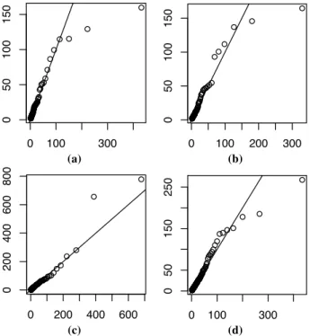
Fig. 5.Simulated data: QQplots of the radius variable|r| condition-ally on|r|>µ. The x-axis corresponds to the true quantiles while the y-axis represents the estimated quantiles. See the caption of Fig. 3 to understand the meaning of the four different panels.
Eq. (8), respectively. As expected, the dependence among low and medium values generated by the Gamma density does not play a strong role in the upper tail. This explains the small difference in the histogram shapes between the up-per and lower panels. The dissimilarity between the left and right panels is due to the strong disparity in the extreme be-havior dependencies captured by the coefficientsβ1andβ2. Figure 4 compares the estimation result forσ=0.9 andξ=0.8 from 50 realizations of length 1000 from our mixture model with a strong dependence in its core and tail. The so-called “1D Frigessi 1” and “1D Frigessi 2” case corresponds to the boxplots obtained whenR1andR2are wrongly assumed to be independent. The boxplot “2D Frigessi” displays the esti-mation result when the correct model is assumed. In this lat-ter case, the true values ofσandξare correctly estimated and the uncertainty spreads are reasonable. In contrast, wrongly assuming independence ofR1andR2clearly underestimates the true value ofσ andξ and increases the boxplots width. This shows that applying a classical univariate approach and ignoring the dependence can mislead the practitioner.
Overall, Figs. 3 and 4 indicate three things: (1) our model is able to generate different types of dependencies in the up-per tail, (2) the low and medium values do not influence the overall shape dependence in the extremes, and (3) our esti-mation procedure seems to work adequately.
Concerning the intensity of the extremes produced by our model and obtained by our estimation algorithm, we can
ob-0.0 0.2 0.4 0.6 0.8 1.0
0.0 0 .2 0.4 0 .6 0.8 1 .0 1.2 1 .4
0.0 0.2 0.4 0.6 0.8 1.0
0.0 0 .5 1.0 1 .5 2.0 2 .5 3.0 (a) (b)
Fig. 6. Observed rainfalls: Histograms of theωvalues condition-ally on|r|>µˆ for the two weather stations pairs: Panel (a) the “St-Alban-Perreux” couple and Panel (b) the “Perreux-Riorges” pair. The solid lines correspond to the fitted Beta distributions.
serve Fig. 5 that displays four QQplots from our four sam-ples. The x-axis corresponds to the true quantiles while the y-axis represents the estimated quantiles. These graphs in-dicate that very large extreme values can be adequately re-produced, e.g. see Panel (c). Still, the performance varies from samples to samples. For example, the largest value in Panel (a) is underestimated. Overall, the four fitted QQplots seem to capture most of the extreme behaviors. In order to confirm this result and to provide GPD goodness-of-fit tests, Andersen-Darling A2 and Cram´er-von Mises W2 statistics were computed (e.g. Choulakian and Stephens, 2001). Both statistics show that the GPD fits can be considered as accept-able for a confidence level of 99% (i.e. with p-values<0.01). Although this simulation study is limited to only four cases, the discrepancy among the four studied situations seems to indicate that our estimation procedure can cover a wide range of dependence cases, and therefore it can now be applied to real precipitation data.
4.3 Precipitation measurements
5 10 15 20 25
5
1
0
1
5
2
0
2
5
3
0
3
5
GPD quantiles
C=r1+r2 data quantiles
10 20 30 40 50
10
20
30
40
GPD quantiles
C=r1+r2 data quantiles
(a) (b)
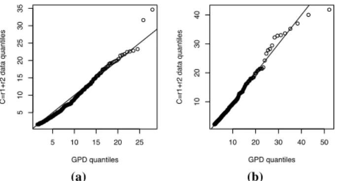
Fig. 7. Observed rainfalls: QQplots of the observed|r|quantiles conditionally on|r|>µˆ vs. estimated GPD quantiles for each pair: (a) corresponds to the couple “St-Alban-Perreux”, (b) to “Perreux-Riorges”.
dependence has already been observed in the bottom panel of Fig. 1. Panel (a) of Fig. 6 is more difficult to interpret. The histogram, as well as the Beta fit, seems to indicate a mild dependence, much weaker than in panel (b), but this is not the U-shape that characterizes the independence, e.g. the left panels of Fig. 3. Concerning large precipitation intensi-ties, the QQplots in Fig. 7 indicate a good agreement between the estimated and observed quantiles for the two pairs of stations. The GPD goodness-of-fit tests performed through Andersen-Darling A2 and Cram´er-von Mises W2 statistics (see Choulakian and Stephens, 2001), show that, as for sim-ulated data, the GPD fits are considered as acceptable for a confidence level of 99% (i.e. with p-values<0.01), confirm-ing the QQplots.
5 Conclusions and perspectives
We have presented a new statistical distribution that can model the entire range (i.e. low, medium and extreme val-ues) of bivariate precipitation measurements. This model consists in a mixture between a bivariate Gamma distribu-tion – representing the precipitadistribu-tion density core (i.e. the non extreme part) – and a product of GP and Beta densities in a Pickland’s coordinates system – characterizing heavy rainfall density. The mixture is weighted through a function varying with the extremes strength within each pairwise rainfall data. A simulation scheme and an estimation procedure have been proposed and tested. Four simulated samples have been gen-erated and studied. The dependence structure as well as the parameter values have been correctly retrieved for each sim-ulated sample. Our estimation procedure has been applied to real precipitation measurements from three weather sta-tions located in the South of France. Our statistical model-ing confirms that nearby stations provide dependent record-ings, not only for mean precipitation values but also among heavy rainfalls. This suggests that past studies that have com-pletely ignored the spatial dependence between weather
sta-tions may have led to imprecise statistical outputs, specially in terms of extreme value analysis. More research is needed to extend our pairwise rainfall model into a fully multivari-ate framework. Besides the estimation problem beyond the 2-D case, the difficulty resides in proposing a parsimonious model that can be based on multivariate EVT and also offer enough flexibility to represent the dependencies within small precipitation, heavy rainfalls and between both.
Acknowledgements. This work was supported by the european E2-C2 grant, the National Science Foundation (grant: NSF-GMC (ATM-0327936)), by The Weather and Climate Impact Assessment Science Initiative at the National Center for Atmospheric Research (NCAR) and the ANR-AssimilEx project. The authors would also like to credit the contributors of the R project.
Edited by: B. D. Malamud
Reviewed by: two anonymous referees
References
Akaike, H.: A new look at the statistical model identification, IEEE Transactions on Automatic Control, 19, 716–723, 1974. Beirlant, J., Goegebeur, Y., Segers, J., and Teugels, J.: Statistics of
Extremes: Theory and Applications, Wiley Series in Probability and Statistics, 2004.
Carreau, J. and Bengio, Y.: A hybrid Pareto model for asymmet-ric fat-tail data, Technical report 1283, Dept. IRO, Universit´e de Montr´eal, 2006.
Choulakian, V. and Stephens, M. A.: Goodness-of-fit Tests for the Generalized Pareto Distribution, Technometrics, 43, 478–484, 2001.
Coles, S. G.: An introduction to statistical modeling of extreme values, Springer Series in Statistics, 2001.
Cooley D., Nychka, D., and Naveau, P.: Bayesian Spatial Model-ing of Extreme Precipitation Return Levels, J. Am. Stat. Assoc., 102(479), 824–840, 2007.
De Haan, L. and Ferreira, A.: Extreme Value Theory: An Intro-duction, Springer Series in Operations Research and Financial Engineering, 2006.
Embrechts, P., Kl¨uppelberg, C., and Mikosch, T.: Modelling Ex-tremal Events for Insurance and Finance, Applications of Math-ematics, vol. 33, Springer-Verlag, Berlin, 1997.
Fisher, R. A. and Tippett, L. H. C.: Limiting forms of the frequency distribution of the largest or smallest member of a sample, Pro-ceedings of the Cambridge Philosophical Society, 24, 180–190, 1928.
Frigessi, A., Haug, O., and Rue, H.: A dynamic mixture model for unsupervised tail estimation without threshold selection, Ex-tremes, 5, 219–235, 2002.
Katz, R., Parlange, M., and Naveau, P.: Extremes in hydrology, Adv. Water Resour., 25, 1287–1304, 2002.
Katz, R. W.: Precipitation as a chain-dependent process, J. Appl. Meteorol., 16, 671–676, 1977.
Naveau, P., Nogaj, M., Ammann, C., Yiou, P., Cooley, D., and Jomelli, V.: Statistical methods for the analysis of climate ex-tremes, C. R. Geoscience, 337, 1013–1022, 2005.
Resnick, S.: Heavy-Tail Phenomena: Probabilistic and Statistical Modeling, Springer Series in Operations Research and Financial Engineering, 2007.
Schwarz, G.: Estimating the dimension of a model, Ann. Statist., 6, 461–464, 1978.
Vrac, M. and Naveau, P.: Stochastic downscaling of precipita-tion: From dry events to heavy rainfalls. Water Resour. Res., 43, W07402, doi:10.1029/2006WR005308, 2007.
Vrac, M., Stein, M., and Hayhoe, K.: Statistical downscaling of pre-cipitation through a nonhomogeneous stochastic weather typing approach. Climate Research, 34, 169–184, doi:10.3354/cr00696, 2007.