Luciana P. Bassi Marinho* Institute of Aeronautics and Space São José dos Campos - Brazil [email protected] Ana Cristina Avelar Institute of Aeronautics and Space São José dos Campos - Brazil [email protected] Gilberto Fisch Institute of Aeronautics and Space São José dos Campos - Brazil [email protected] Suelen T. Roballo National Institute for Space Research São José dos Campos - Brazil [email protected] Leandro Franco Souza University of Sao Paulo São Paulo - Brazil [email protected] Ralf Gielow National Institute for Space Research São José dos Campos - Brazil [email protected] Roberto da Mota Girardi Technological Institute of Aeronautics São José dos Campos - Brazil [email protected] *author for correspondence
Studies using wind tunnel to
simulate the Atmospheric
Boundary Layer at the Alcântara
Space Center
Abstract: The Alcântara Space Center (ASC) region has a peculiar topography
due to the existence of a coastal cliff, which modifies the atmospheric boundary layer characteristic in a way that can affect rocket launching operations. Wind tunnel measurements can be an important tool for the understanding of turbulence and wind flow pattern characteristics in the ASC neighborhood, along with computational fluid dynamics and observational data. The purpose of this paper is to describe wind tunnel experiments that have been carried out by researchers from the Brazilian Institutions IAE, ITA and INPE. The technologies of Hot-Wire Anemometer and Particle Image Velocimetry (PIV) have been used in these measurements, in order to obtain information about wind flow patterns as velocity fields and vorticity. The wind tunnel measurements are described and the results obtained are presented.
Key words: Alcântara Space Center (ASC), Particle image velocimetry,
Turbulence, Wind flow, Wind tunnel.
LIST OF SYMBOLS INTRODUCTION
Wind regimes and atmospheric turbulence in the boundary ALA Aerodynamics Division
layer have been object of great interest in Aerospace ASC Alcântara Space Center
Meteorology. Serious rocket launch failures, for example, ACA Atmospheric Science Division
two Titan 34Ds, an Atlas Centaur, a Delta, two Arianes and a AEB Brazilian Space Agency
Columbia, occurred between 1985 and 2003. Several of AT Anemometer Tower
these losses have been weather-related. In the case of CNPq National Council for Scientific and
Challenger, for example, the main cause was the failure of Technological Development
the Solid Rocket Booster (SRB) joint, caused in part by the IAE Institute of Aeronautics and Space
very low temperatures experienced. IBL Internal Boundary Layer
INPE National Institute for Space Research
However, it has been argued that upper-wind conditions at ITA Technological Institute of Aeronautics
launch time were a significant contributing factor, since VLS Satellite Launcher Vehicle
severe shear-induced turbulence may well have reopened a PIV Particle Image Velocimetry
transient SRB metal seal (Baker, 1986). According to MIT Mobile Integration Tower
Kingwell et al. (1991), the main meteorological factors that Reδ Reynolds Number based on the coastal cliff
affect rocket operations are lightning, since electrical height SRB - Solid Rocket Booster
surges can trigger loss of control and make rockets lose
u∞ Streamwise wind speed
control and be destroyed; temperature and humidity fields,
δ Coastalcliff height
that affect the formation of fog and ice on the vehicle;
____________________________________
Received: 13/05/09 turbulence, that can impose unacceptable stresses on key
vehicles, and wind, that can affect the electronic guidance experiments that have been carried out in cooperation system. among researchers from IAE, ITA and INPE. These experiments have been implemented using technologies such as Hot-Wire Anemometry and Particle Image Knowledge about wind flow patterns and atmospheric
Velocimetry (PIV) in a wind tunnel, in order to investigate turbulence are important to provide basic information for
the wind flow pattern and turbulence at the ASC, where Research & Development (R&D) since the rockets are
abrupt changes in surface roughness exist. Computational designed to withstand loads due to the wind, and also
Fluid Dynamics (CFD) was also used in these trajectory, control and guidance are determined by the
investigations.
profile of wind near the surface. According to Fisch (1999), up to the height of 1000 m, 88 per cent of the trajectory corrections are due to the wind, while above 5000 m, this influence is only 3 per cent. In the particular case of the Brazilian Satellite Launcher Vehicle, (VLS), which is a four-stage rocket, it suffers lateral deviation in its trajectory, later compensated by the guidance system.
Sounding rockets, as they are smaller, are more affected in their trajectory by thewind flow pattern. Therefore, their take-off velocity (ballistic wind lower than 6.0 m/s) is relatively small, and produces important changes in the launch azimuth due to the lateral wind speed component (Marques and Fisch, 2005). In addition, the rockets can be also affected by turbulence when positioned at the ramp, prior to the launch. Wind data is usually obtained from meteorological stations, and vertical profile measurement devices, such as anemometric towers or masts, give details of the wind in certain places. However, valuable
information can be obtained from wind tunnel experiments Figure 1: General view of Alcântara Space Center
about the modification of the atmospheric boundary layer caused by abrupt changes in local topography.
Recently, wind tunnels have been used in Micrometeorology Science due to their advantage of flow control. Recent studies can be found in the literature, for example, Novak et al. (2000) analyzed the turbulent structure of the atmosphere within and above canopy. Simulations of the atmospheric wind field at a complex topography were conducted in order to plan the Naro Space Center at South Korea (Kwon et al., 2003). Studies on pollutant dispersion immersed in obstacles were carried out by Mavroidis and Griffiths (2003), and simulations of the air flow for complex topography were carried out by Cao and Tamura (2006).
The Brazilian Rockets, such as the VS-40, and VSB-30 . sounding rockets, and the VLS, have been launched from .
the Alcântara Space Center (ASC), which is located on the Figure 2: Detailed view of the MIT in the ASC. coast of Maranhão State, at the latitude 2° 19' S, longitude
44° 22' W, 40m above sea-level and a distance of 30 km
from São Luiz. As can be observed in Fig. 1, there is a Alcântara Space Center characteristics coastal cliff along the shoreline in the ASC neighborhood.
Consequently, in addition to an abrupt change in roughness Because of the ASC's peculiar topographical from the smooth oceanic surface to a rugged continental characteristics, the wind, initially in balance with the terrain, a topographical variation of 40 m is added. oceanic surface, interacts with the low woodland vegetation (average height of the trees is 3m), modifying itself with the formation of an Internal Boundary Layer (IBL). A The Mobile Integration Tower (MIT) is located 150 m from
schematic representation of the IBL development as it the edge of this coastal cliff. Figure 2 shows the area of the
moves over a smooth surface (ocean) and then across a ASC, the anemometer tower (AT) and the MIT.
The terrain's influence on the flow downstream from the wind predominates approximately up to 5000 m, with wind cliff surface depends not only on its characteristics, but also speeds of 7.0 ~ 8.0 m/s at levels between 1000 and 3000 m. on the characteristics of the previous surface, upstream the In the dry season, the wind is predominantly from east, and cliff, over which the flow was in balance. So, a new reaches up to an altitude of approximately 8000 m, with equilibrium layer is formed, the vertical thickness of which wind speeds of 7.0 ~ 9.0 m/s, being particularly strong in the increases with the distance from the edge. Above this new layer up to 2000 m, with averages between 10.0 and 10.5 layer the wind profile remains in balance with the previous m/s, and manifesting a small south-easterly rotation. This surface, while within it, the wind profile is adjusted to the shift occurs due to intensification of the sea breeze, which new surface (Stull, 1988). displays its maximum impact (ocean-continent thermal contrast) during this period, particularly from September to November. Air temperature and the relative humidity do not present seasonal variations and their values are typical of the tropical atmosphere due to its geographic location (Fisch, 1999).
BACKGROUND
The Atmospheric Science Division (ACA) conducts studies concerned with the atmospheric systems that occur at the ASC. In cooperation with the Aerodynamics Division (ALA) activities have begun related to the understanding of the atmospheric turbulence at the ASC using wind tunnels in another scientific project related to the upgrading of
Figure 3: IBL development from a smooth surface to a rough
instrumentation and modernization of the aerodynamic
surface (adapted from Savelyev and Taylor, 2005).
tunnel TA-2 in order to simulate the atmospheric boundary layer. The objectives are to use TA-2 with a modern PIV system to simulate the flow at the ASC for a Reynolds The classical work of Elliot (1958) and the following
6
number around 10 . The TA-2 wind tunnel is a facility of the theoretical and experimental studies carried out by
al ALA and is Brazil's biggest aerodynamic wind tunnel. Pendergrass and Arya (1984), Sempreviva et . (1990),
Sugita and Brutsaert (1990), Källstrand and Smedman
Description of the experiments
(1997) and Jegede and Foken (1998) focused on the neutral flow problem that occurs due to the change in roughness. In
The wind tunnel experiments were carried out at the Prof. these studies, the development of the modified wind flow
Kwein Lien Feng Laboratory at the Institute of pattern, the IBL growth and the turbulent field implications
Aeronautical Technology, (ITA), using an open circuit, were investigated. Slvelvev and Taylor (2005) did a very
closed jet subsonic wind tunnel with a square test section detailed review of published formulas following on from
(465 mm x 465 mm) 1200 mm in length. The maximum Elliot's pioneering work. According to Jegede and Foken
wind speed through the test section is 33 m/s. (1998), non-neutral situations can be represented by
adjusting empirical coefficients of the neutral cases.
The atmospheric flow field was simulated by prolonging Subsequently, thermal stratification effects on wind flow
the test section, and by installing a screen and some spires as pattern and IBL growth were introduced, as shown by
al represented in Fig. 4. These spires consist of triangular steel Batchvarova and Gryning (1998), Liu et . (2000), and
al plates, which were positioned at the entrance of the Hara et . (2009). It should be mentioned that atmospheric
measurement chamber and combined with the roughness stability at the ASC can be considered to be neutral due to
(felt carpet with a thickness of 3 mm was used) to produce the high winds. Loredo-Souza (2004) took wind tunnel
the boundary layer profile similar to the atmospheric wind measurements showing that atmospheric stability can be
flow (Santa Catarina, 1999). considered neutral if the wind speed is around 10 m/s. This
is the case of the ASC (Roballo and Fisch, 2008). The
Average wind speed values and fluctuations were obtained vegetation in the ASC area is characteristic of a region of
through hot-wire anemometer measurements. A schematic “restinga”. Average height of the vegetation is around 3 m.
design of measurements using the hot-wire anemometry The climate presents a precipitation regime divided into
technique is represented in Fig. 5. A coordinate system (x,y) two periods: (i) a wet period, with heavy rains from January
was used as a reference system, where the negative x values to June, with March and April receiving the peak rainfalls,
correspond to the ocean (upwind of the cliff) and the with monthly totals above 300 mm; and (ii) a dry period,
positive x values correspond to the continent (downwind). from July to December, with precipitation lower than 15
mm per month (Fisch, 1999).
A two-dimensional PIV system was used to obtain air flow velocity fields. PIV is a very important experimental tool There are marked differences in the wind regime between
allows instantaneous and non-intrusive measurement of the images were processed using the adaptive-correlation flow velocity, ranging from micro PIV to large industrial option of the commercial software developed by Dante wind tunnel applications. As opposed to the more Dynamics (Flow Manager 4.50.17). A 32 pixels × 32 pixels commonly used single-point measurements, PIV allows the interrogation window with 50 per cent overlap and moving spatial structure of the velocity field to be visualized as well average validation was used.
as quantified. A good description of this technique is given
by Raffel et al. (2007). The basic principle of this technique To enable the boundary layer formation in the region of involves photographically recording the motion of optical access, and to allow PIV measurements, in addition microscopic particles that follow the fluid flow. to devices such as the spires and carpet, a screen was also
used, as represented schematically in Figure 4.
The experimental results were compared with numerical results obtained from the computational code named
Immersed Boundary developed by Góis (2007) and Pires (2009).
Figure 4: Apparatus used for the experiments.
(a)
Figure 6: PIV system installed in the wind tunnel test section.
(b) One of the models used to simulate the ASC and the MIT (represented by a wooden block of dimensions 10 x 10 x 50 mm) is represented in Fig. 7. In order to simulate the irregularity of the coastal cliffs, experiments were made with varying inclinations. These models were painted in flat black to avoid laser reflections.
Figure 5: Overhead view of the experimental design with the
coordinates x (longitudinal) and y (lateral).
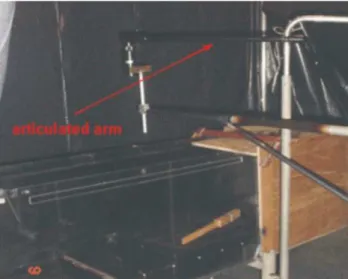
To conduct the experiments, the wind tunnel test section flow was seeded with smoke particles, approximately 5mm in diameter, using a Rosco Fog generator. A New Wave Nd-YAG 200 mJ dual pulsed Nd:Yag laser, with a repetition rate of 15 Hz, was employed to illuminate the flow field. A vertical laser sheet was created using an articulated arm, as shown in Fig. 6, and a set of lenses for laser thickness adjustment. A 60 mm diameter Nikon lens was fitted to a 12-bit high-resolution digital camera HiSense 4M (built by Hamamatsu Photonics, Inc.) with acquisition rate of 11 Hz, spatial resolution of 2048 × 2048 pixels and 7.4 m pixel
Comparison between experimental and numerical simulation results
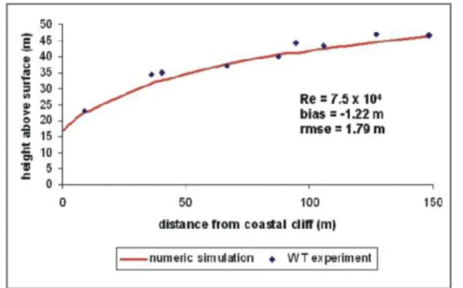
Figure 8 shows a comparison between IBL height obtained from the wind tunnel experiments, for Reynolds Number
4
based on the coastal cliff height (δ), Reδ, equal to 7.2 x 10 , and the IBL height obtained from numerical simulation. For the numerical simulation and for the wind tunnel measurements, the coastal cliff was taken to be 40m in height and perpendicular to the wind direction. In the numerical simulation, a 2D model was used, with vorticity-velocity formulation. High-order compact finite-difference schemes were adopted for the derivative approximations,
th
and a 4 order Runge-Kutta method was used to integrate time (Góis, 2007). The coastal cliff was specified through the immersed boundary method (Pires, 2009). More details about this methodology can be obtained from Pires et al. (2009). A strong correlation between the numerical and experimental results was observed, providing a validation of the numerical method adopted.
Figure 8: The IBL results from wind tunnel measurements and numerical simulation.
The streamwise wind speed (u∞) ranged from 27 to 30m/s corresponding to a Reδ, based on the height of the coastal
4 4
cliff of 40 m varying from 7.2 x10 to 8 x 10 . These were the maximum Reδ, values obtained in this wind tunnel. In the
6 7
atmosphere, the Reδ is basically of the order of 10 and 10 .
Figure 9: Average velocity profile (a) and fluctuating velocity
profiles (b) along the central lane.
RESULTS
Figure 10 presents turbulent intensity obtained with the Figure 9 presents the wind speed profiles (or velocity) and
wind speed and deviation measured at the heights the fluctuation (or deviation) of the wind along the central
corresponding to the levels of the anemometric tower (e.g. lane (keeping the position y = 0 in Fig. 5). It is possible to
6, 10, 16.3, 28.5, 43 and 70 m). It is possible to observe that observe the modification of the profiles at the cliff (position
turbulent intensity is higher close to the ground surface,
x = 0). Also, it can be noticed that the wind speed values are
specially close to the discontinuity, reaching values of 0.7 at lower after the cliff, associated with the higher values of the
level 1. There is also a significant decrease in turbulent fluctuation, mainly close to the surface. This is an indication
intensity with height and at level 6 (equivalent to 70 m of the turbulence, due to the step, up to a distance around
height) the turbulent intensity is around 0.1 for all positions 300 mm from the discontinuity (cliff). The bigger
along the central line. The distance of 300 mm is estimated fluctuation values for a non-dimensional height lower than
as the distance where the turbulence caused by the edge 0.2 represents the influence of the surface, which creates
Figure 11: Wind profile, stream lines (a) and the vorticity (b).
Figure 10: Turbulence Intensity distribution along the central lane (position y = 0).
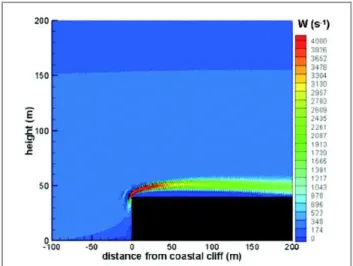
Figure 12 shows the vorticity obtained numerically. It should be noted that this simulates the real case with Reδ =
7
2.0 x 10 . It should also be noted that the higher the Re the Figure 11 shows the wind profile, the stream lines and the
lower the IBL height. (Pires, 2009) wind vorticity obtained from the wind tunnel
measurements. The geometric structure of the coastal cliff affects the height of the IBL reaching the MIT.
It is possible to observe the formation of a strong recirculation zone downwind of the coastal cliff as described before. Theoretically, the IBL height is zero at the usual change of surface roughness. However, in this present case, the coastal cliff (40 m) causes an initial height for IBL at the discontinuity (x = 0), which is in the range of 7 to 10m.
-1
The wind vorticity (Fig. 11b) ranging from -1600 to 300 s was generated for the experiments in the wind tunnel. In
-1
each case a wind vorticity equal to 300 s is generated by the flow when reaching the MIT and a negative vorticity (-
-1
1600 s ) is generated above the coastal cliff and the MIT (Pires, 2009).
Figure 12: Vorticity obtained in numerical simulation to Reδ =
7
2.0 x 10 .
CONCLUDING REMARKS
ACKNOWLEDGMENTS Estimates”, Boundary Layer Meteorology, Vol. 85, pp. 1-33
L.B.M. Pires is grateful for support received from CNPq Kingwell, J., Shimizu, J., Narita, K., Kawabata, H., and CAPES, and S.T. Roballo for her Doctoral and Master Shimizu, I., 1991, “Weather Factors Affecting Rocket of Science fellowships at INPE. G. Fisch is thankful for the Operations: A Review and Case History”, Bulletin support from CNPq (throughout Research Scholarship American Meteorological Society, Vol. 72, No. 6, pp. 778-302117/2004-0), L.F. Souza acknowledges the support of 793.
FAPESP (process 04/16064-9). The authors would like to
thank the technicians José Rogério Banhara and José Kwon, K. J., Lee J. Y., Sung, B., 2003, “PIV Measurements Ricardo Carvalho de Oliveira, both from the Aerodynamics on the Boundary Layer Flow Around Naro Space Center”, Division, ALA, for their valuable help in this research. In: 5th International Symposium on Particle Image Velocimetry, Busan, Korea. PIV'03 Paper 3121, Busan, Korea.
REFERENCES
Liu, H.; Chan, J. C. L., Cheng, A. Y. S., 2000, “Internal Baker, D., 1986, “Why Challenger Failed”, New Scientist, Boundary Layer Structure Under Sea-breeze Conditions in pp. 52-5, 11 sep. Hong Kong”, Atmospheric Environment, Vol. 35, pp.
683-692. Batchvarova, E., Gryning, S. E., 1998, “Wind Climatology,
Atmospheric Turbulence and Internal Boundary-Layer Marques, R. F. C., Fisch, G., 2005, “As Atividades de Development in Athens During the Medcaphot-Trace Meteorologia Aeroespacial no Centro Técnico Aerospacial Experiment”, Atmospheric Environment, Vol.32, No. 12, (CTA)”, Boletim da Sociedade Brasileira de Meteorologia. pp. 2055-2069. A Meteorologia e a Aeronáutica, Vol. 29, No. 3, pp. 21-25. Cao, S., Tamura, T., 2006, “Experimental Study on Mavroidis, I., Griffiths, D. J. H., 2003, “Field and Wind Roughness Effects on Turbulent Boundary Layer Flow Tunnel Investigations of Plume Dispersion Around Single Over a Two-dimensional Steep Hill”, Journal of Wind Surface Obstacles”, Atmospheric Environment, Vol. 37, Engineering and Industrial Aerodynamics. No. 1,Vol. 94, No. 21, pp. 2903-2918.
pp. 1-19.
Novak, M. D., Warland, J. S., Orchansky, A. L., Ketler, R., Elliott, W. P., 1958, “The Growth of the Atmospheric Green, S., 2000, “Wind Tunnel and Field Measurements of Internal Boundary Layer”, Transactions, American turbulent flow in forests. Part I: Uniformly Thinned Geophysical Union, Vol.39, No. 6, pp. 1048-1054. Stands”, Boundary Layer Meteorology. Vol.95, No. 3, pp.
457-495. Fisch, G., 1999, “Características do Perfil Vertical do Vento
no Centro de Lançamento de Foguetes de Alcântara
Pendergrass, W., Arya, S. P., 1984, “Dispersion in Neutral (CLA)”, Revista Brasileira de Meteorologia, Vol. 14, No. 1,
Boundary Layer Over a Step Change in Surface Roughness pp. 11-21.
I. Mean Flow and Turbulence Structure”, Atmospheric Enviroment, Vol. 18, pp. 1267-1279.
Góis, E. R. C., 2007, “Simulação Numérica do Escoamento em Torno de Um Cilindro Utilizando o Método das
Pires, L. B. M., 2009, “Estudo da Camada Limite Interna Froenteiras Imersas”, Dissertação (Mestrado em Ciência da
Desenvolvida em Falésias com Aplicação para o Centro de Computação e Matemática Computacional) - Universidade
Lançamento de Alcântara”, 150f. Tese (Doutorado em de São Paulo, São Carlos.
Meteorologia) National Institute for Space Research, São José dos Campos.
Hara, T., Ohya, Y., Uchida, T., Ohba R., 2009, “Wind-Tunnel and Numerical Simulations of the Coastal Thermal
Pires, L. B. M., Souza, L. F., Fisch, G. E., Gielow, R., 2009, Internal Boundary Layer”, Boundary-Layer Meteorology,
“Numerical Study of the Atmospheric Flow Over a Coastal Vol.130, pp. 365-381.
Cliff”, International Journal Numerical Methods in fluids (submitted in corrections).
Jegede, O. O., Foken, T., 1998, “ A Study of the Internal Boundary Layer Due to a Roughness Change in Neutral
Raffel, M., Willert, C., Wereley, S., Kompenhans J., 2007, Conditions Observed During the LINEX Field
“Particle Imaging Velocimetry; A Practical Guide”, Campaigns”, Theoretical and Applied Climatology, Vol.
Springer, Berlin Heidelberg New York. 62, pp. 31-41.
Roballo, S. T., 2007, “Estudo do Escoamento Atmosférico Källstrand, B., Smedman, A. S., 1997, “A Case Study of the
no Centro de Lançamento de Alcântara (CLA) Através de Near-neutral Coastal Internal Boundary-layer Growth:
130f. Dissertação (Mestrado em Meteorologia) National Institute for Space Research, São José dos Campos.
Roballo, S. T.;, Fisch, G., 2008, “Escoamento Atmosférico no Centro de Lançamento de Alcântara (CLA): Parte I - Aspectos Observacionais”, Revista Brasileira de Meteorologia, Vol. 23.
Santa Catarina, M. F., 1999, “Avaliação do Escoamento no Centro de Lançamento de Foguetes de Alcântara: Estudo em Túnel de Vento”, 72f. Relatório Final de Atividades de Iniciação Cientifica, Instituto Tecnológico de Aeronáutica, São José dos Campos, Brazil.
Savelyev, S. A., Taylor, P. A., 2005, “Internal Boundary Layers: I. Height Formulae for Neutral and Diabatic Flows”, Boundary Layer Meteorology, Vol. 115, pp. 1-25. Sempreviva, A. M., Larsen, S. E., Mortensen, N. G., Troen, I., 1990, “Response of Neutral Boundary Layers to Change of Roughness”, Boundary-Layer Meteorology, Vol. 50, pp. 205-225.
Stull, R., 1988, “An Introduction to Boundary Layer Meteorology”, London: Kluwer.