DOI: http://dx.doi.org/10.1590/2446-4740.03815
*e-mail: [email protected]
Received: 04 December 2015 / Accepted: 23 August 2016
Comparative study of periodicity estimation methods using ultrasonic
signals
Adriana Kauati*, Wagner Coelho de Albuquerque Pereira, Marcello Luiz Rodrigues Campos
Abstract Introduction: Various signal-processing techniques have been proposed to extract quantitative information about internal structures of tissues from the original radio frequency (RF) signals instead of an ultrasound image. The quantiiable parameter called the mean scatterer spacing (MSS) can be useful to detect changes in the quasi-periodic microstructure of tissues such as the liver or the spleen, using ultrasonic signals. Methods: We evaluate and compare the performance of three classic methods of spectral estimation to calculate the MSS without operator intervention: Tufts-Kumaresan, SAC (Spectral Autocorrelation) and MUSIC (MUltiple SIgnal Classiication). Initially the evaluations were performed with 10,000 signals simulated from a model in which the variables of interest are controlled, and then, real signals from sponge phantoms were used. Results: For the simulated signals, the performance of all three methods decreased with increasing Ad or jitter levels. For the sponges, none of the methods accurately estimated the pore size. Conclusion: For the simulated signals, Tufts-Kumaresan had the lowest performance, whereas SAC and MUSIC had similar results. For sponges, only Tufts-Kumaresan was able to detect the increase in the size of the pores of the sponge, although most often, it estimated sizes larger than expected.
Keywords: Mean spacing, Ultrasonic scatterers, Spectral estimation, Periodic media.
Introduction
Ultrasound is a well-established method of medical imaging, which uses non-ionizing radiation and has a low cost of implementation. However, the ultrasound image is usually interpreted visually and qualitatively. Conventional ultrasound images (grayscale) are formed from echoes that return from the irradiated structures. These images represent
specular relections from interfaces between different
acoustic impedance structures and backscattered echoes from the interaction between the ultrasound
and microstructures. Specular relections indicate the
contours of organs, vessels, cysts, and macroscopic structures in general, while scattering generates the gray
granulation (speckle) that ills the interiors of organs
and tissues. These images provide a visualization of anatomical structures in motion in real time, but the more subtle changes in tissue microstructure, such
as the early stages of cirrhosis or ibrosis or fetal maturation are dificult to identify visually (Shung and Thieme, 1993).
Various signal-processing techniques have been proposed to extract quantitative information of internal structures of tissues obtained from the original radio frequency (RF) signals, such as: acoustic speed (Bamber and Hill, 1981; Bouzitoune et al., 2016), backscatter
coeficient (Bamber and Hill, 1981; Bouzitoune et al.,
2016; Lu et al., 1991), spectral slope (Bouzitoune et al., 2016) and attenuation coeficient (Bamber and Hill, 1981; Bouzitoune et al., 2016; Lu et al., 1991) and the Mean Scatterer Spacing (MSS).
MSS represents the spatial organization and is therefore of particular interest for detecting changes in tissue that have quasi-periodic microstructures, such as the liver or spleen tissue (Fellingham and Sommer, 1984). To this end, various techniques of power spectrum and cepstrum (power spectrum of the logarithm of the power spectrum) several techniques have been proposed for estimating MSS such as the ones described by: Fellingham and Sommer (1984), Narayanan et al. (1997) and Wear et al. (1993). The studies of Varghese and Donohue (1993, 1994, 1995) were based on spectral autocorrelation, and Simon et al. (1997) proposed an algorithm to estimate the MSS based on the spectral redundancy generated by an RF signal quadratic transformation. All these techniques are applied to RF signals or their envelope, which contains a mixture of contributions from periodic and non-periodic scatterers.
Using human calcanei, Pereira et al. (2004) estimated MSS using Singular Spectral Analysis and concluded it may be useful for providing information associated with tissue microarchitecture. In 2006
Machado et al. (2006) studied in vitro the periodicity of human liver tissue and found that MSS alone could not characterize tissues, concluding that additional parameters are needed to improve its accuracy. Also using human tissue, Huang et al. (2008) wrote an article estimating the mean spacing within trabecular bone
using a simpliied inverse ilter-tracking algorithm
and concluded it has the potential to be a method for estimating average spacing in low signal-to-noise environments with large spacing variations.
In 2011, Chen et al. (2011) proposed a time-frequency approach to estimate the MSS. They used simulated and real backscattered echoes of liver tissues in vivo and concluded that their method is potentially superior to Simon’s (1997), avoiding false peaks in the spectrum. More recently, Pan et al. (2015) proposed a Golay code-based cepstrum estimation and the results show that the method is robust against noise.
Comparing the techniques, Kauati et al. (2012) evaluated the Burg, Wiener, and MUSIC (MUltiple
SIgnal Classiication) spectral estimation methods to
calculate the MSS (without operator intervention). Initially the evaluation was performed using 10,000 simulated signals with the aim of studying each method’s behavior using a model in which the variables of interest can be controlled. Then, the methods were applied to real signals of nylon phantoms immersed in water. The Burg method could not estimate the spacing of phantom signals, presenting results similar to the other methods only for simulated signals. The Wiener method for simulated signals was second best in terms of percentage of success. When considering the phantom signals, the MUSIC method had the best performance of all three methods.
In this work, we will compare the MUSIC method, which had the best performance in Kauati et al. (2012), with two other methods also used to estimate periodicity: Tufts-Kumaresan and SAC (Spectral Autocorrelation).
Methods
In this section, the equations and algorithms of the MUSIC, Tufts-Kumaresan and SAC methods will be presented. The study was initially performed using simulated ultrasonic (US) signals based on a linear model of US interaction with biological tissue, in order to have more control of the variables involved. Then, we used real signals from sponge phantoms immersed in water. Examples of both kinds of signals (simulated and real) will also be presented. The approaches used to evaluate the methods, the phantoms used to generate the real
signals, and the signal treatments proposed in this work will be described at the end of this section.
Supporting methods
Tufts-Kumaresan
Based on modiied covariance, Tufts and Kumaresan (1982) determined a prediction ilter of N samples in the forward and backward directions, and the prediction equations can be written in matrix form as:
1
2
3
( ) ( 1) (1) ( 1)
( 1) ( ) (2) ( 2)
( 1) ( 2) ( ) ( )
* (1) * (2) * ( ) * (1)
* (2) * (3) * ( 1) * (2)
* ( ) * ( 1) * ( ) * ( )
y L y L y y L
y L y L y y L
g g
y N y N y N L y N
y y y L y
g
y y y L y
y N L y N L y N y N L
− + + + − − − = − + − − + − (1)
where, y(n): input signal; g: ilter impulse response; L: predictor ilter order; N: number of samples. In other words,
Ag = –h (2)
where, A: matrix formed by the input signal; h: vector formed by the input signal.
Thus, g is given by
g = –A#h (3)
where, A#: pseudoinverse of A#.
The correlation matrix R can be calculated by:
R = A * A (4)
Where, * is the transpose of the complex conjugate.
The correlation vector is deined by
r = A * h (5)
and the prediction ilter g can be calculated as
g = R#r (6)
The Tufts-Kumaresan ilter is deined as
gtk = [1 g] (7)
The ilter order is crucial to the frequency estimation
performance. According to Tufts and Kumaresan (1982)
the best order is deined by the window size minus the
number of periodicities in the signal divided by two. The Tufts-Kumaresan method, with values of example parameters, is presented below. The size
a few windows of different sizes and by checking which one had the best result.
1. Given:
• window size = 200 points. • number of periodicities = 1
• order of the ilter = window size - number
of periodicities
• overlap = half of the window size
2. Thus, for each window, we calculate the matrix A and h, according to Equation 1, for the RF signal envelope.
3. The vector g will be calculated for each window as: g=( * ) (A A# −A h* )
4. At the end, we calculate the average of g with all windows
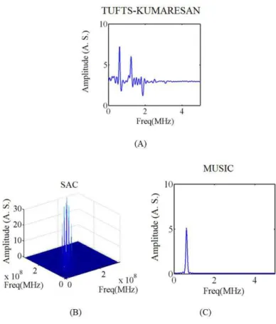
5. From the ilter gtk frequency response, we
can ind the frequency within the speciied
window that presents the largest amplitude value. This will be the requested frequency (Figure 1A).
SAC
The SAC (Spectral Autocorrelation) method performs an analysis on the spectrum calculated by:
*
1 2 1 2
( , ) ( ). ( )
S f f =Y f Y f (8)
being: ( )
Y f =Fourier transform of the envelope RF signal *
( )
Y f =Conjugate of the Fourier transform of the envelope RF signal
The relative frequency of the mean spacing of regular scatterers is determined by the off-diagonal dominant peak, which is equivalent to the PSD. The analysis outside the main diagonal was used, because according to Varghese and Donohue (1993), the expected value of diffuse component is zero in this region.
The steps for the implementation of SAC method can be summarized as follows:
1. Calculate the FFT of the envelope of the RF signal and its conjugate.
2. Calculate the product of both of them (Equation 8).
3. Normalize through the main diagonal. 4. Remove the main diagonal.
5. The frequency related to the position of maximum amplitude in the spectrum is the one related to MSS (Figure 1B).
MUSIC
The MUSIC (MUltiple SIgnal Classiication)
method (Marple, 1987) is based on obtaining the matrix eigenvalues and eigenvectors formed by covariances according to equation:
[
]
11 2 1
( ) i i N i N y y
c i y y y
y + − + = ×
(9)
where, c (i) = matrix elements; Y= original signal. From a generic estimator of frequencies:
( )
( ) 2
1 1 p H k k k M P f
e f a
= +
= α
∑ (10)
being, ak = eigenvector; eH = eigenvector hermitian
transposed; αk = weight.
The estimator of frequencies of MUSIC is based on the noise subspace eigenvectors with uniform weight, so the frequency regarding the mean spacing
of scatterers is deined by the point of maximum
amplitude in the MUSIC spectrum.
( ) ( ) ( ) 1 1 MUSIC p H H k k k M P f
e f a a e f
= + = ∑ (11)
where e f( ) is a vector formed by:
1 exp( 2 ) ( )
exp( 2 )
j fT e f
j fMT
π
=
π
(12)
where, T is half the period limited by the analysis window for M eigenvectors forming the signal space.
The steps for the MUSIC method implementation can be summarized as follows:
1. Draw the MUSIC spectrum according to Equation 11, considering the RF signal envelope.
2. The frequency related to the position of maximum amplitude in the spectrum is the one related to MSS. (Figure 1C).
Signals used in the analysis
Simulated tissue
The RF signals simulated in this study followed the model used by Maciel (2000) of backscattered echoes, considering a one-dimensional medium and linear behavior. Thus, the echo signal received as a function of time, r(t), can be written as:
( ) ( ) * ( ) ( )
r t =p t g t +n t (13)
where, p t( )= transmitted ultrasound pulse; g t( )= function of characterization of medium (Impulse Response);
( )
n t = experimental system noise; * = convolution.
The function g(t) can be modeled as the sum of echoes scattered by each mediumparticle where a group of particles has a regular spatial distribution (periodic) and the other group has an irregular distribution (aperiodic):
( ) ( ) ( )
1 1
N M
i i i i
i i
g t c t b t
= =
=∑ δ − τ +∑ δ − θ (14)
where: N = total number of regular particles; M = total
number of dispersed particles; ci = regular signal amplitude;τi = regular part delay (regarding the position); bi = dispersed signal;θi= dispersed part delay (regarding the position);δ = impulse function.
This model is compatible with biological tissues that have regular structures mixed with diffuse ones, such as liver tissue, and is similar to the ones found in the literature.
Evaluation
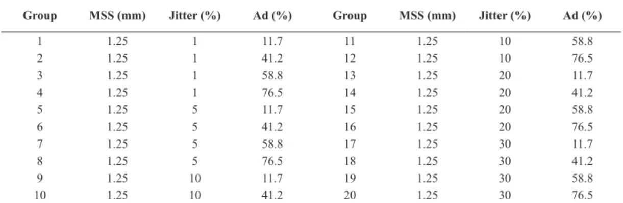
First, the methods were evaluated using 10,000 signals simulated with different levels of Ad (the ratio between the echoes’ mean amplitudes from the diffuse and regular particles) and jitter (percentile variance of mean space between the regularly spaced particles). The signals were divided into 20 groups of 500, according to the characteristics in Table 1. The sampling frequency was 25 MHz, the transducer excitation frequency was 20 MHz, and the excitation signal band was 1.5 MHz.
The signals were simulated with MSS = 1.25 mm
(compatible with the biological tissues), whose frequency related to periodicity (FreqMSS) is calculated according to the following equation:
2
c FreqMSS
MSS
=
⋅ (15)
where, FreqMSS = frequency of maximum magnitude; c = ultrasound velocity; MSS = mean scatterer spacing.
Figure 2 shows signal sections: (A) Ad = 11.7%
and jitter = 1%, (B) Ad = 11.7% and jitter = 30%, and (C) Ad = 76.5% and jitter = 1%. It can be seen that the intervals become progressively more dificult to be visually identiied.
Sponge phantom
central frequency and bandwidth of 20 MHz to acquire the backscattered RF signals. The sponges were placed with the surface parallel to the scanning plan (Figure 3). The ampliied RF signal was scanned with an 8-bit resolution oscilloscope (details on Table 2) (Pereira et al., 2002).
Figure 4 shows a section of each sponge signal with different spacing. Each of the 176 signals for each
sponge was reduced to 512 points, a size suficient to
identify frequencies of the expected order of magnitude.
Signal treatment
To evaluate the three methods, all the signals were
iltered by a Butterworth ilter of order 6, with cutoff
frequencies related to spacings of 0.02 mm (38.5 MHz) to 3.00 mm (256.67 kHz) for sponge signals, and 0.10 mm (7.70 MHz) to 5.00 mm (154.00 kHz) for the simulated signals. Cutoff frequencies were calculated for each signal part depending on the estimated US speed. For these values, the speed used was 1540 m/s (average speed for biological tissues).
Table 1. Characteristics of simulated signals.
Group MSS (mm) Jitter (%) Ad (%) Group MSS (mm) Jitter (%) Ad (%)
1 1.25 1 11.7 11 1.25 10 58.8
2 1.25 1 41.2 12 1.25 10 76.5
3 1.25 1 58.8 13 1.25 20 11.7
4 1.25 1 76.5 14 1.25 20 41.2
5 1.25 5 11.7 15 1.25 20 58.8
6 1.25 5 41.2 16 1.25 20 76.5
7 1.25 5 58.8 17 1.25 30 11.7
8 1.25 5 76.5 18 1.25 30 41.2
9 1.25 10 11.7 19 1.25 30 58.8
10 1.25 10 41.2 20 1.25 30 76.5
Figure 2. Examples of simulated signals with MSS = 1.25mm: (A) Ad = 11.7% and jitter = 1% (B) and Ad = 11.7% and jitter = 30% (C)
As the RF signal envelope has the same properties as the RF signal average spacing (Maciel, 2000), the analysis was performed only on the envelope so that it is more robust in estimating the periodic component. The signal envelope was calculated as the analytic signal obtained using an RF signal Hilbert transform, subtracting the average (to remove the DC level), and dividing by the variance for the energy normalization.
Results
For the three methods studied, an initial analysis using 10,000 simulated signals with various levels of Ad and jitter combined was performed. By using such a signal model, it was possible to control the signal characteristics independently. Sponges, which mimic the almost quasi-periodic spacing of tissues, were used to obtain signals closer to real biological tissues.
For the simulated signals, Figure 5 presents the results for the percentage of correct estimates for different levels of Ad. For each method, different curves
are presented with a tolerance range of 10% around
the value of the correct frequency in the simulated spacing – in this case, 616.00 kHz, in a medium with a US speed of 1.540 m/s. It was observed that for all methods the performance decreased with the increase of Ad or jitter levels, as expected.
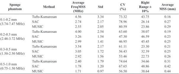
The summarized results for the four phantoms for the three methods are presented in Table 3. The mean velocity for each sponge was obtained as the estimated mean velocity. Their values were 1.494 m/s sponge
0.1-0.2 mm 1.486 m/s sponge 0.2-0.3 mm, 1.499 m/s sponge 0.3-0.5 mm and 1.494 m/s for the sponge of 0.5 to 1.0 mm (Pereira et al., 2002).
Discussion
For the simulated signals the Tufts-Kumaresan method had the lowest performance, whereas SAC and MUSIC obtained similar results. It can be noted from Figure 5 that each method maintains a reasonable precision percentage even when the average amplitude
of the aperiodic signal is about 40% of the average amplitude of the periodic signal (Ad = 41.2%) and jitter reached 10%. From this point, performance
rapidly deteriorates indicating that the frequency is no longer evident. It is important to note that for the simulated signals, the dominant feature is the use of frequencies with greater or lesser amount of associated
noise. In real cases, there are large isolated relectors
and/or highly attenuating structures that generate more complex signals.
For sponges, only the Tufts-Kumaresan method was able to identify an increase in the size of pores (frequency decreases as the size of pores increases), although it estimated higher frequencies than expected.
No outlier was excluded, although they clearly exist. If there was such an exclusion, the results would be closer to the expected values. This technique was used by some authors, such as Pereira et al. (2002).
It should be noted that the sponges do not have a preferred frequency, but a distribution of unknown frequencies. It is also observed that the sponges are composed of structures with various shapes and
thicknesses, which cause a variation in the relected
energy that make up the backscattering signal under study.
The results with simulated signals show that SAC and MUSIC are potential methods to estimate the MSS. Figure 3. RF signal acquisition set-up using a commercial transducer (model M316; 3.2-mm diameter, Panametrics, Waltham, MA) with central frequency and bandwidth of 20 MHz.
Table 2. The sponge phantom with respective sampling rate.
Sponges Sampling rate
Pores between 0.1 and 0.2 mm 100 MHz
Pores between 0.2 and 0.3 mm 100 MHz
Pores between 0.3 and 0.5 mm 250 MHz
Figure 4. Examples of signals of 4 sponge phantoms (A) spacing between 0.1 and 0.2 mm; (B) spacing between 0.2 and 0.3 mm; (C) spacing between 0.3 and 0.5 mm and (D) spacing between 0.5 and 1.0 mm.
Figure 5. Results for simulated signals for the methods: (A) Tufts-Kumaresan; (B) SAC; and (C) MUSIC for a range of tolerance of 10%
Table 3. Results for four different sponge phantoms for the three methods for a US speed in the medium of 1.494 m/s.
Sponge
phantom Method
Average FreqMSS
(MHz)
Std CV
(%)
Right Range ±
10%
Average MSS (mm)
0.1-0.2 mm (3.74-7.47 MHz)
Tufts-Kumaresan 4.56 3.34 73.32 43.75 0.16
SAC 2.74 2.17 78.96 26.14 0.27
MUSIC 2.55 2.05 80.59 23.86 0.29
0.2-0.3 mm (2.48-3.72 MHz)
Tufts-Kumaresan 4.00 2.54 63.60 38.07 0.19
SAC 3.26 1.54 47.30 46.59 0.23
MUSIC 2.99 1.41 46.95 45.45 0.25
0.3-0.5 mm (1.50-2.50 MHz)
Tufts-Kumaresan 3.54 2.17 61.11 23.30 0.21
SAC 3.05 1.72 56.43 32.39 0.25
MUSIC 2.92 1.56 53.46 22.73 0.26
0.5-1.0 mm (0.75-1.50 MHz)
Tufts-Kumaresan 2.40 1.79 74.64 34.66 0.31
SAC 1.78 1.20 67.65 48.86 0.42
MUSIC 1.71 0.97 56.50 38.64 0.44
Regarding sponge phantoms, SAC and MUSIC were able to estimate MSS values inside the periodicity range for one sponge (2nd sponge), while Tufts-Kumaresan
estimated values inside the periodicity range only once (1st sponge). However, Tufts-Kumaresan was the only
method able to estimate progressively higher MSS values; hence, it was able to sense the increase in the pore sizes of the sponges. A more detailed study is needed to investigate the sensibility of each method and their contour conditions.
References
Bamber JC, Hill CR. Acoustic properties of normal and cancerous human liver-I: dependence on pathological condition. Ultrasound in Medicine & Biology. 1981; 7(2):121-33. http:// dx.doi.org/10.1016/0301-5629(81)90001-6. PMid:7256971.
Bouzitoune R, Meziri M, Machado CB, Padilla F, Pereira WCA. Can early hepatic fibrosis stages be discriminated by combining ultrasonic parameters? Ultrasonics. 2016; 68:120-6. http://dx.doi.org/10.1016/j.ultras.2016.02.014. PMid:26945441.
Chen SP, Tsao S, Tsao J. A joint time-frequency approach to mean scatterer spacing estimation. In: Proceedings of the 4th International Conference on Biomedical Engineering and Informatics; 2011 Oct 15-17; Shanghai. USA: IEEE; 2011. 602-6. http://dx.doi.org/10.1109/BMEI.2011.6098431.
Fellingham L, Sommer F. Ultrasonic characterization of tissue structure in the in vivo human liver and spleen. IEEE Transactions on Sonics and Ultrasonics. 1984; SU-31(4):418-28. http://dx.doi.org/10.1109/T-SU.1984.31522.
Huang K, Ta D, Wang W, Le LH. Simplified inverse filter tracking algorithm for estimating the mean trabecular bone spacing. IEEE Transactions on Ultrasonics, Ferroelectrics, and Frequency Control. 2008; 55(7):1453-64. http://dx.doi. org/10.1109/TUFFC.2008.820. PMid:18986934.
Kauati A, Pereira WCA, Campos MLRC. Detecção automática do espaçamento médio de meios periódicos por sinais ultrassônicos retroespalhados. Revista Brasileira de
Engenharia Biomédica. 2012; 28(3):261-71. http://dx.doi. org/10.4322/rbeb.2012.033.
Lu ZF, Zagzebski JA, Lee TF. Ultrasound backscatter and attenuation in human liver with diffuse disease. Ultrasound in Medicine & Biology. 1991; 25:1047-57.
Machado CB, Pereira WCA, Meziri M, Laugier P. Characterization of in vitro healthy and pathological human liver tissue periodicity using backscattered ultrasound signals. Ultrasound in Medicine & Biology. 2006; 32(5):64957. http://dx.doi.org/10.1016/j. ultrasmedbio.2006.01.009. PMid:18285062.
Maciel CD. Análise de espectro singular aplicada a sinais ultra-sônicos [dissertation]. Rio de Janeiro: Universidade Federal do Rio Janeiro; 2000.
Marple SL. Digital spectral analysis: with applications. New Jersey: Prentice-Hall; 1987.
Narayanan VM, Molthen RC, Shankar PM, Vergara LJ, Reid M. Studies on ultrasonic scattering from quasi-periodic structures. IEEE Transactions on Ultrasonics, Ferroelectrics, and Frequency Control. 1997; 44(1):114-24. http://dx.doi. org/10.1109/58.585205. PMid:18244109.
Pan W, Shen Y, Liu T, Wang Y. Golay improvement of the robustness of mean scatterer spacing measurement with ultrasonic backscattering. Bio-Medical Materials and Engineering. 2015; 26(s1 Suppl 1):455-65. http://dx.doi. org/10.3233/BME-151335. PMid:26406037.
Pereira WCA, Abdelwahab A, Bridal SL, Laugier P. Singular spectrum analysis applied to 20MHz backscattered ultrasound signals from periodic and quasi-periodic phantoms. Acoustical Imaging. 2002; 26:239-46. http://dx.doi.org/10.1007/978-1-4419-8606-1_31.
Pereira WCA, Bridal SL, Coron A, Laugier P. Singular spectrum analysis applied to backscattered ultrasound signals from in vitro human cancellous bone specimens. IEEE Transactions on Ultrasonics, Ferroelectrics, and Frequency Control 2004; 51(3):302-12. http://dx.doi.org/10.1109/ TUFFC.2004.1320786. PMid:15128217.
Simon C, Shen J, Seip R, Ebbini ES. A Robust and computationally efficient algorithm for mean scatterer spacing estimation. IEEE Transactions on Ultrasonics, Ferroelectrics, and Frequency Control. 1997; 44(4):882-94. http://dx.doi.org/10.1109/58.655203.
Tufts DW, Kumaresan R. Estimation of frequencies of multiple sinusoids: making linear prediction perform like maximum likelihood. Proceedings of the IEEE. 1982; 70(9):975-89. http://dx.doi.org/10.1109/PROC.1982.12428.
Varghese T, Donohue KD. Characterization of tissue microstructure scatterer distribution with spectral correlation. Ultrasonic Imaging. 1993; 15(3):238-54. http://dx.doi. org/10.1177/016173469301500304. PMid:8879094.
Varghese T, Donohue KD. Estimating mean scatterer spacing with the frequency-smoothed Spectral autocorrelation function. IEEE Transactions on Ultrasonics, Ferroelectrics, and Frequency Control. 1995; 42(3):451-63. http://dx.doi. org/10.1109/58.384455.
Varghese T, Donohue KD. Mean scatterer spacing estimate with spectral correlation. The Journal of the Acoustical Society of America. 1994; 96(6):3504-15. http://dx.doi. org/10.1121/1.410611. PMid:7814765.
Wear KA, Wagner RF, Insana MF, Hall TJ. Application of autoregressive spectral analysis to cepstral estimation of mean scatterer spacing. IEEE Transactions on Ultrasonics, Ferroelectrics, and Frequency Control. 1993; 40(1):50-8. http://dx.doi.org/10.1109/58.184998. PMid:18263156.
Authors
Adriana Kauati1*, Wagner Coelho de Albuquerque Pereira2, Marcello Luiz Rodrigues Campos3
1 Laboratory of Instrumentation and Biomedical Engineering, Centro de Engenharias e Ciências Exatas – CECE,
Universidade Estadual do Oeste do Paraná – UNIOESTE, Avenida Tarquinio Joslin dos Santos, 1300, Polo Universitário, CEP 85870-650, Foz do Iguaçu, PR, Brazil.
2 Biomedical Engineering Program, Instituto Alberto Luiz Coimbra de Pós-graduação e Pesquisa em Engenharia –
COPPE, Universidade Federal do Rio de Janeiro – UFRJ, Rio de Janeiro, RJ, Brazil.
3 Electrical Engineering Program, Instituto Alberto Luiz Coimbra de Pós-graduação e Pesquisa em Engenharia – COPPE,