ISSN 0104-6632 Printed in Brazil
Brazilian Journal
of Chemical
Engineering
Vol. 20, No. 04, pp. 391 - 401, October - December 2003
THE THREE-DIMENSIONAL NUMERICAL
AERODYNAMICS OF A MOVABLE
BLOCK BURNER
T.J.Fudihara
1, L.Goldstein Jr.
1*and M.Mori
21
Thermal and Fluids Engineering Department, School of Mechanical Engineering, State University of Campinas, P.O. Box 6122, 13.083-970, Campinas - SP, Brazil.
E-mail: [email protected]
2
Chemical Processes Department, School of Chemical Engineering, State University of Campinas, P.O. Box 6066, 13.081-970, Campinas - SP, Brazil.
E-mail: [email protected]
(Received: November 25, 2002 ; Accepted: June 3, 2003)
Abstract. Computational fluid-dynamics techniques were employed to study the aerodynamics of a movable block swirl burner, developed by the International Flame Research Foundation, IFRF, which is characterized by the ability to adjust continuously and dynamically the intensity of the swirl by means of the simultaneous rotation of eight movable blocks, inserted between eight fixed blocks. Five three-dimensional grids were
constructed for the burner, corresponding to five positions of the movable blocks. Both the k-ε and RNG k-ε
isotropic turbulence models were applied. Only the latter described the existence of a central reverse flow along the annular duct. The employment of first-order and second-order interpolation schemes provided distinct results. The later provided results closer to the experimental tests. The swirl number decayed in the annular duct. The predicted swirl numbers for this movable block swirl burner were lower than the corresponding IFRF’s experimental data, as was also observed by other researchers. This gave rise to the suspicion of some possible measurement error in the IFRF’s experiments. On the other hand, the lack of agreement between the experimental data and the predictions regarding swirling flows could be attributed to
the possible inadequate performance of the k-ε model, as a consequence of its isotropic approximation. Still
another possible explanation could be a phenomenon called bifurcation, in which one given swirl number can be associated with two distinct conditions of steady state flow. In addition, this complex flows requires a scrupulous development of the grids for the boundary condition and the employment of adequate interpolation schemes.
Keywords: burner, swirling flows, turbulence models, CFD, finite volume.
INTRODUCTION
Burners are the main operational devices in furnaces. They control the various physical and chemical processes that develop in a combustion chamber, such as the mixing of the reagents and the generation of combustion products or free radicals, the latter of which are actively involved in the formation of soot due to their high level of reactivity. In addition, they define the distribution of residence
times of chemical compounds and the extension of the circulation regions that affect flame stability. They also act as liquid fuel atomisers, determining the characteristics of the drops. This variety of functions results from their control over the flux and the trajectory of the reactants, which emerge in the combustion chamber as a high velocity jet.
classified as those that channel the flow or those that employ rotating mechanical devices. In the first method, which is more common in practice, are found those burners that use channels tangential to the inlet duct, or use restrictions like, for example, a set of blades inside the flow path, which orient and generate the swirl. In the other class, the rotating devices transfer movement to the flows upon contact by a vane or even a rotating duct, which rotates on its axis, with the stream flowing inside it.
Beér and Chigier (1974) proposed an approximate analytical correlation to calculate the swirl number of the burners that use flow channelling, by guidance blades or movable blocks, to generate swirl. These correlations were derived from geometrical relations and were submitted to several simplifications relative to the nature of the flow.
In a numerical and experimental study of another IFRF rotating flow burner, a guide blades in cascade-type burner, Widmann et al. (2000) obtained by simulation a swirl number which was about half of that obtained from the Beér and Chigier’s approximate analytical correlation for this burner, which they corroborated with their own experiments. They concluded that the simplifications embedded in the correlation were inadequate. In addition, the
authors compared the k-ε and the RNG k-ε
turbulence models, where the latter achieved better agreement with the experimental data. They foresaw a reverse flow in the core of the burner exit using the RNG k-ε model. The renormalization group theory (RNG) was primarily developed for the quantum field theory, and latter applied in the derivation of the RNG k-ε turbulence model (Yakhot & Orszag, 1986, and Yakhot & Smith, 1992). Constants of the ε equation were obtained by the renormalization group method, in contrast to the empirical constants of the standard k-ε model. Morvan et al. (1998) listed a
series of advances achieved by the RNG k-ε
turbulence model, as in the description of flows with both high and low Reynolds numbers, and in swirling or circulation flows. On the other hand, Launder and Spalding (1974) suggested that the poor performance of the k-ε model was a consequence of its isotropic approximation, who had observed that the k-ε model did not represent adequately the swirling flows, and pointed out the superiority of the nonisotropic models, such as the Reynolds-stress model, which would be noticeable in spite of its complexity and computational cost.
Generally, a simplified boundary condition is assumed for the combustion chamber as a substitute
for the burners, for it has the advantage of allowing that a more refined grid be used. This idealization could well, as was suggested by Dong and Lilley (1994) and Xia et al. (1997), be the reason of the distortions found in the results, rather than the utilization of an isotropic turbulence model, especially with swirling flows. On the other hand, in a numerical simulation corroborated by experiments, Guo et al. (2001) obtained good approximations using the k-ε model in a swirling flow. The authors observed a complex and transient behaviour in spiral, despite the fact that the boundary configuration was only a duct where the velocity components were fixed.
Jiang and Shen (1994) attributed the failure of the predictions regarding swirling flows much more to a phenomenon called bifurcation than to the k-ε turbulence model. In the bifurcation phenomenon one given swirl number can be associated with two distinct conditions of steady state flow. This phenomenon of non-unique steady-state behaviour occurs as a consequence of two paths through which the desired swirl number can be obtained, that is by the gradual increase in the intensity of the swirl, the lower branch, or, alternatively, by the gradual reduction in the intensity of the swirl from a higher condition, the upper branch. They observed the existence of a bifurcation in the curve of the ratio of the maximum flow rate in the external reverse zone (ERZ) by that in the internal reverse zone (IRZ) as a function of the swirl number, such that, the predicted swirl number can differ significantly from the experimental swirl number depending on the path.
All authors seem to agree that a first-order numerical interpolation scheme is insufficient.
The objective of this work was to analyze these various related questions, by comparing the results of a three-dimensional numerical simulation to the available experimental data of a movable block swirl burner.
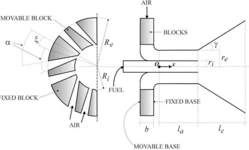
THE MOVABLE BLOCK BURNER
In this burner, eight fixed blocks and eight movable blocks are placed alternately at the entrance section between the internal and external radii (Ri
and Re, respectively), as shown in Figure 1. The
angle between the surface of a block and an imaginary plane that passes through the axis of the burner and intersects the surface at Ri, defines the
so that the variations in time can be perceived, results in the basic equations that describe the process. The time averages are implicit in all primitive variables in the equations that follow. block has an oblique surface and another of α equals
to zero, so that the combustion air enters both radially and tangentially through the openings between the blocks. The aperture angle, ξ, of an oblique opening is determined by the angle between two imaginary planes that cross the axis and intersect the two edges of the breach at Ri, where ξm is the
maximum aperture angle possible. The blocks are uniformly distributed so that all the oblique openings as well as all the normal openings have the same aperture angle. Due to the simultaneous movement of the movable blocks, alternating with the fixed blocks, when the oblique passages are opened, the non-oblique passages are closed and vice versa, increasing or reducing the intensity of the swirl of the air flow. After a 90° curve, the air converges into the annular duct. It was assumed that the cylindrical internal duct, used to injection of fuel, was closed at its external extremity in order to reproduce the experiments presented by Beér and Chigier (1974).
Continuity Equation
.( ) 0
t
∂ρ+ ∇ ρ =
∂ v (1)
Momentum Equation
.( ) P
t
.( ) B
∂ρ + ∇ ρ = −∇ + ∂
′ ′ +∇ υ − ρ +
v
vv v v
(2)
where:
T
2
( ( ) 3
υ= ϕ− µ ∇⋅ δ + µ ∇ + ∇v v v ) (3)
MATHEMATICAL MODELLING The Reynolds stress, ′ ′ v v
ρ , that appeared during the averaging was not null and must be modelled. The eddy viscosity hypothesis has been used to derive various turbulence models, including the k-ε and RNG k-ε models. In the Reynolds-stress model, on the other hand, the eddy viscosity hypothesis is not used and its components must be solved individually. More details about these models can be found in Garde (1994) and Lixing (1993).
The turbulence phenomena are inherent to the processes involved in this study. Their modelling is inserted in the transport equations by the Reynolds decomposition and averaging method. Applying a time averaging procedure to the continuity and momentum equations at a time interval which is high enough for the averaged values of the instantaneous fluctuation to be considered null, but small enough
Eddy Viscosity Hypothesis where: According to this hypothesis, the Reynolds stress
is modelled by: S
(
ef2
k
3
)
Π = Π − ∇ ⋅ µ ∇ ⋅v v +ρ (11)
( )
(
T)
S ef
Π = µ ∇ ⋅ ∇v v + ∇v (12)
( )
(
)
T T T 2 2 k . 3 3 ′ ′−ρ = − ρ δ − µ ∇ δ +
+µ ∇ + ∇
v v v
v v
(4)
and ν is the equivalent Prandtl number.
Substituting it into Equation 2, results:
RNG k-ε TURBULENCE MODEL
(
)
( )
(
T)
ef B P t +
∂ρ + ∇⋅ ρ = −∇ +′
∂
+∇⋅ µ ∇ + ∇
v
vv
v v
(5) in the same way as in the former model (Equation 8). In this model, the turbulent viscosity is calculated
The fields of the k and ε variables were obtained from the following equations of Yakhot & Orszag (1986) and Yakhot & Smith (1992):
where P’ is defined as:
(
)
TkRNG k k k t µ
∂ρ +∇⋅ ρ −∇⋅ µ+∂ ν ∇ =
= Π − ρε
v (13) ef 2 2 k 3 3
P P ρ + µ − ϕ ∇ ⋅
′ = + v (6)
and the effective viscosity as:
and T
ef
µ = µ + µ (7)
(
)
(
)
T
RNG
2
1RNG k 2RNG k
.
C C C
t
ε Π η µ
+∇⋅ ρ ε −∇ µ +ν ∇ε =
ε ε
= − − ρ
∂ρε
∂ v (14)
The turbulent viscosity, µT, is calculated
following the initial proposal of Kolmogorov and Prandtl as:
2 T
k Cµ
µ = ρ
ε (8) where:
0 3 RNG 1 C 1 η
η η −
η
=
+ β η (15)
where k is the kinetic turbulent energy, ε is its dissipation rate, and Cµis a constant.
k-ε TURBULENCE MODEL
0,5 S
T
k
Π η = µ ε
(16)
Of the various two-equation models of turbulence developed during the past decades, the k-ε model has been the most frequently used. In order to obtain µT,
additional equations for k and ε should be solved: βand C1kε, C2kε, C3kε, C1RNG, C2RNG, νk,νε, νkRNG, νεRNG,
RNG and η0 are the model constants.
(
k)
T kk t κ ∇ µ
∂ρ +∇⋅ ρ −∇⋅ µ+∂ v ν = Π −ρε (9)
SWIRL NUMBER, S
and The intensity of the swirl of the flow in the burner
can be associated with a dimensionless parameter, the swirl number, defined as:
( )
(
)
T 1k 2k k.
t
C
C
εεΠ ε
µ
∂ρε ∇⋅ ρ ε −∇ µ+
∂
ν
∇ε =
ε
=
−
ρε
+
v
(10)
w u e
G S
G r
where is the axial flux of the angular momentum, is the axial flux of the axial momentum and r
w G
u
G e is
the nozzle radius of the burner.
The axial flux of the angular and the axial momenta can be obtained by integration of the functions that describe the angular velocity, w, the axial velocity, u, and the static pressure, P, by:
r w
0
G
= π
2
∫
(wr)
ρ
u
r dr
(18)and (19)
r u
0
G
= π
2
∫
u
ρ
ur dr
+ π
2
∫
dr
r 0
Pr
Due to the fact that obtaining the static pressure is not an easy task, its omission from the axial flux in the axial momentum equation results in an approximate value of the swirl number, defined as S’. This simplification was explored by Widmann et
al. (2000), who claimed that when the pressure term in the axial flux of the axial momentum equation was preserved, a much lower swirl number resulted.
Beér and Chigier (1974) proposed an approximate analytical equation for the swirl number, from the hypothesis of uniform distribution of the axial velocity, and the assumption that the reduction of the angular momentum in the burner duct beyond the swirler was negligible:
2
' e i
e r r
S 1
2b r
= σ − (20)
where σ is the ratio of the mean tangential velocity by the radial velocity at the burner exit, which was obtained analytically for the movable block burner. Recently Beér (2002) informed the need to correct a printing error in the equation for σ whose denominator should be squared, so that:
( )
( )
m 2m
m
cos 1 tan tan 2
2 sen z
1 1 cos 1 tan tan 2
ξ ξ
α + α ξ
π
σ = α
ξ ξ ξ
− − α + α
ξ
(21)
NUMERICAL METHODS
The transport equations were solved by the finite volume method in a generalized co-ordinate system with collocated variables in a structured grid, using the CFX, version 4, computational software. The pressure velocity coupling was solved by the SIMPLEC algorithm. All simulations were carried out by the second-order higher-order upwind differencing interpolation scheme according to the Guidelines of the CFX-4 (2001), using the previous results of the first-order upwind differencing scheme as a start-up, due to its better convergence performance. The steady-state solution was reached using the false time-step method. The flow was
assumed to be isothermal and incompressible. More details about these methods and techniques can be found in Patankar (1980) and Maliska (1995).
In the construction of the numerical grid, which can be observed in Figure 2, it was not necessary to represent the movable or the fixed blocks, but only the breaches between them, through which the air flowed. Five grids for the aperture fractions, ξ/ξm, of 0, 0.25, 0.5, 0.75 and 1 were
developed, and their external surfaces are shown in Figure 3. Nearly 52800 control volumes were employed for aperture fractions of 0 and 1, and 90700 control volumes for the others. Burner dimensions, for which variables were shown in Figure 1, are presented in Table 1.
Table 1: Geometric parameters of the burner.
Variables
ri (m) 30. 10-3
re (m) 95. 10-3
Ri (m) 165. 10-3
Re (m) 264. 10-3
b (m) 65. 10-3
la (m) 160. 10-3
lc (m) 190. 10-3
α (degree) 50
γ (degree) 35
ξm (degree) 12
Figure 2: Numerical grid for the aperture fraction of 0.5.
ξ
/
ξ
m= 0
ξ
/
ξ
m= 0.25
ξ
/
ξ
m= 0.5
ξ
/
ξ
m= 0.75
ξ
/
ξ
m= 1
Operational and Numerical Boundary Conditions
The same relative uniform pressure was fixed at all inlets, and kin was estimated from
2 in
0.002v and εin
from k1,5in 0.3d (Khalil et al., 1975), where vin is the inlet
velocity and d is the inlet hydraulic diameter. The analyses were grouped according to two mass flow rates fixed at the outlet: 1300 kg/h and 2000 kg/h, defined as the mass flow rate boundary condition. The velocity field in the cells close to the stagnant condition on the wall was obtained using the wall-function method, assuming the stress strain as constant in the layer from the wall to the centre of those cells, where the velocity have a logarithmic profile (Launder and Spalding, 1974).
RESULTS AND DISCUSSION
The predicted values of S’ at the exit of the annular cylindrical duct, at the junction with the expansion, are shown in Figure 4 for the two mass flow rates used with the higher-order upwind differencing scheme. They didn’t show dependence on the mass flow rate and were only a function of the opening fraction of the oblique inlet, ξ/ξm; this
agrees with the experimental data presented by Beér and Chigier (1974) for the movable block burner.
For the higher values of S’, when ξ/ξm was 0.75
or 1, the higher-order upwind scheme showed more stable convergence and better corroboration with the experimental data than those obtained with the upwind scheme. When the swirl was weaker, as when ξ/ξm was 0 or 0.25, the numerical instability
was greater than that observed with the upwind scheme, perhaps reflecting the physical phenomenon itself. No preferential flow direction was observed;
the flow behaved in an unstable manner, and did not have a defined path. This was observed when the simulation was performed with a transient regime instead of the false time-step method, even with the upwind scheme which has the characteristic of attenuating the oscillations. The phenomenon seemed to be intensified by the expansion at the exit of the annular duct. The situation when S’ is zero for an ξ/ξm of zero, as is shown in Figure 5, can occur
only at sporadic and undetermined moments.
The swirl numbers S’ calculated from the approximate analytical correlation for σ appeared well adjusted to the available IFRF experimental data, but the predicted swirl numbers remained well below the approximate analytical curve, as can be seen in Figure 5. As observed previously, one should be careful with the printing error found recently in Beér and Chigier’s correlation for σ. Most authors attributed the deviations mainly to the use of isotropic turbulence models. However, another possible explanation could be the intrusive presence of a probe, which probably was used in the acquisition of the experimental data, or the existence of the bifurcation phenomenon associated with swirling flows, as was previously noted.
According to Shtern and Hussain (1996), there would exist four kinds of jump transitions between steady solutions, resulting in non-unique steady flow regimes for the same control parameters. Jiang and Shen (1994) claimed that it was necessary that the numerical simulations followed a path identical to that in the experiment for a correct corroboration. In the simulations presented it is probable that the lower branch was used; there is no information about that in the experiments report. The presumed effect of multi-stability on the intensity of the swirl, for the same control parameter, is not, however, as yet, well known, and is the object of other studies in progress.
0,0 0,2 0,4 0,6 0,8 1,0
0,0 0,5 1,0 1,5 2,0 2,5 3,0
1300 kg air/h 2000 kg air/h
S'
ξ / ξm
Figure 4: Comparison of the predicted swirl numbers with two mass flow rates for the five aperture
fractions using the RNG k-ε model.
0,0 0,2 0,4 0,6 0,8 1,0
0,0 0,5 1,0 1,5 2,0 2,5 3,0
Upwind
Higher-Order Upwind
Approximate Analytical Curve IFRF Experimental Values
S'
ξ / ξm
Figure 5: Predicted swirl numbers with two interpolation scheme using the RNG k-ε model, and with the Beér
0,00 0,25 0,50 0,75 1,00 0,6
0,8 1,0 1,2 1,4 1,6 1,8 2,0 2,2
ξ/ξm=0,5 ξ/ξm=1,0
S'
x / la
Figure 6: Predicted swirl number decays along the annular region using the
RNG k-ε model.
0,03 0,04 0,05 0,06 0,07 0,08 0,09 0
5 10 15 20 25 30
k-ε RNG k-ε
R
esu
ltan
t V
el
o
cit
y
(
m
/s
)
Radius at x = la (m)
Figure 7: Comparison of the predicted profiles of the mean velocity of the resultant by the k-ε and
the RNG k-ε models.
All the subsequent analysis which follows was conducted with the 1300 kg/h airflow and the higher-order upwind interpolation scheme. Figure 6 shows the simulated S’ values along the annular duct for ξ/ξm
values of 0.5 and 1.0. For a ξ/ξm of 0.5, after the 90°
curve, S’ was approximately 1.0, reducing to 0.66 at the end of the annular duct. For a ξ/ξm of 1.0, the decay
was more severe, going from 2.18 to 1.31. Beér and Chigier’s approximate analytical correlation didn’t foresee this reduction of the swirl number in the annular duct, resulting, in this case, in a difference of up to 65%. Identical decay of the swirl number along the axial direction was observed in the experiments of Edwards et al. (1993), Li and Tomita (1994) and Parchen and Steenbergen (1998) for other rotating flows.
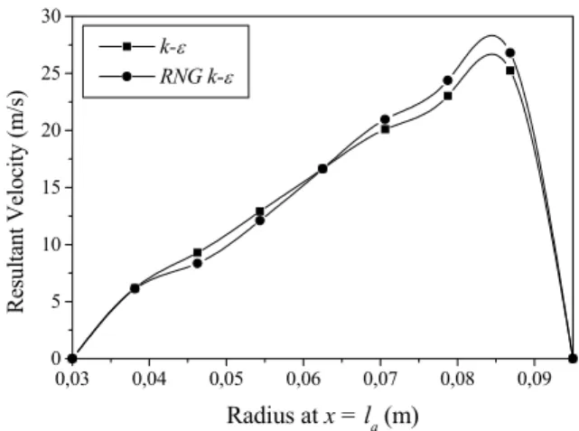
Figure 7 shows a comparison of the mean resultant velocity profiles for a ξ/ξm of 0.5, using the
k-ε and RNG k-ε turbulence models. The differences between both profiles obtained from these models are not easily observed in this figure, but can be seen
when the components of the velocity are compared, as shown in Figure 8, for the k-ε turbulence model, and in Figure 9, for the RNG k-ε turbulence model.
A reverse flow was observed in the expansion, and it was an extension of the internal circulation zone (IRZ) as showed in Figure 10 for the axial velocity. The reverse flow was much more pronounced in the RNG k-ε model, which penetrated almost the entire extension of the annular duct, reaching an axial velocity of - 4 m/s at the annular duct exit and a peak of approximately 22 m/s, in comparison with 19 m/s for the k-ε model. The reverse flow in the annular region was practically imperceptible with the standard k-ε model, and, despite the observations of Jiang and Shen (1994) for rotating flow in a tube expansion, each turbulence model showed distinct results. However, the effects of using the results obtained for the upwind scheme as a necessary initial condition to obtain convergence in the higher-order upwind scheme requires a more extensive investigation.
0,03 0,04 0,05 0,06 0,07 0,08 0,09 -5
0 5 10 15 20 25
radial tangential axial
C
o
m
p
o
n
ent
V
elo
city
(
m
/s
)
Radius at x = la (m)
Figure 8: Predicted profiles of the mean velocity of the components using the k-ε model.
0,03 0,04 0,05 0,06 0,07 0,08 0,09 -5
0 5 10 15 20 25
radial tangential axial
C
om
po
nent
V
el
ocity
(
m
/s)
Radius at x = la (m)
Figure 11 shows the profile of the turbulent kinetic energy, k, and Figure 12, the profile of the dissipation rate of k, ε, at the exit of the annular cylindrical duct, obtained with the k-ε and the RNG k-ε turbulence models. As was observed with the profiles of the mean resultant velocity, the profiles of k were practically identical for the two turbulence models. However, the peak value of ε achieved with the RNG k-ε model was almost 70% greater than that achieved with the k-ε model, at approximately 0.03 m from the external wall, showing the influence of the ε on the definition of the velocity components.
The simulation of the burner provides the information that is necessary for the transient and steady flow regime simulation of a furnace combustion chamber, which can not be accomplished by the usual procedure of using a set of uniform profiles as inlet boundary condition, to represent the burner operation.
One should observe that Beér and Chigier (1974) neglected the pressure term in Equation 19 when definingS′, so that the values of turned out to be much higher than those obtained for S, as was also noted by Widmann et al. (2000).
S′
Figure 10: Maps of the predicted mean axial velocity, vx.
0,03 0,04 0,05 0,06 0,07 0,08 0,09 0
10 20 30 40 50 60 70 80
k-ε
RNG k-ε
k
Radius at x = la (m)
Figure 11: Comparison of the predicted profiles of the turbulent kinetic energy, k, by the k-ε
and RNG k-ε models.
0,03 0,04 0,05 0,06 0,07 0,08 0,09 0
2000 4000 6000 8000 10000 12000 14000 16000
k-ε
RNG k-ε
ε
Radius at x = la (m)
Figure 12: Comparison of the predicted profiles of the dissipation rate of k, ε, by the k-ε
CONCLUSION
A three-dimensional computational simulation was used to study the main characteristics of the flow through a movable block swirl burner developed by the International Flame Research Foundation, IFRF (Beér and Chigier, 1974).
The k-ε and RNG k-ε isotropic turbulence models were applied. Both models predicted a reverse flow in the burner expansion core region, but only the RNG k-ε model predicted a reverse flow extending back into the annular duct of the burner.
The predicted swirl numbers were lower than the available experimental data from the IFRF burner, and lower than an approximate analytical correlation provided for this burner by Beér and Chigier (1974). In a numerical simulation study of a different IFRF type of rotating flow burner, a guide blades in cascade-type burner, Widmann et al. (2000) had already obtained a swirl number S’, corroborated by their own experiments, which was about half of that obtained from Beér and Chigier’s proposed approximate correlation for this burner.
Conversely, the lack of agreement between the experimental data and the predictions regarding swirling flows could be attributed, as mentioned by Jiang and Shen (1994), to the phenomenon of bifurcation, in which one given swirl number can be associated with two distinct conditions of steady state flow. This phenomenon of non-unique steady-state behavior occurs as a consequence of the existence of two paths through which the desired swirl number can be obtained, that is by the gradual increase in the intensity of the swirl, the lower branch, or, alternatively, by the gradual reduction in the intensity of the swirl from a higher condition, the upper branch, such that the predicted swirl number can differ significantly from the experimental swirl number depending on the path.
Another possible explanation is the suggestion of inadequate performance of the k-ε model when applied to a swirling flow, as a consequence of its isotropic nature. This assumption generally came from studies where a simplified boundary condition was assumed for the combustion chamber as a substitute for the burners. But, as was suggested by Dong and Lilley (1994) and Xia et al. (1997), hasty idealizations applied to the boundary conditions could distort the results, especially with swirling flows.
The use of a second-order numerical interpolation scheme produced higher swirl numbers, which were closer to the experimental data than the first-order interpolation scheme. The swirl number decayed
along the axial position, what was not predicted by Beér and Chigier’s approximate analytical correlation.
Publications addressing three-dimensional modeling and simulation of a detailed burner, as the present work, are still scarce. Knowledge of the fluid dynamics of the swirl burners, even in the absence of combustion, is far from absolute.
ACKNOWLEDGEMENTS
The authors are grateful to FAPESP, Fundação de Amparo à Pesquisa do Estado de São Paulo (grant number 00/14390-5), for the financial support that made this work possible.
NOMECLATURE
g gravity vector, m/s2
k turbulent kinetic energy, m2/s2
r nozzle radius, m
t time, s
u axial velocity component, m/s w tangential velocity component, m/s v velocity vector, m/s
z number of fixed or movable blocks
B body force, N/m3
Gu axial flux of the linear momentum
Gw axial flux of the angular momentum
P pressure, N/m2
R radius where the blocks are fitted, m
S swirl number
Constants
Cµ 0.09
C1k-ε 1.44
C2k-ε 1.92
C1RNG 1.42
C2RNG 1.68
β RNG 0.015
η0 4.38
νk 1.00
νε 1.3 νkRNG 0.7179
νεRNG 0.7179
Greek Letters
α inclination angle of the block surface
δ unit tensor
ε dissipation rate of k, m2/s3
ϕ bulk viscosity, kg/m.s
µ molecular viscosity, kg/m.s
ρ density, kg/m3
ξ aperture angle of the oblique inlet
REFERENCES
Beér, J. M., Personal Communication (2002).
Beér, J. M. and Chigier, N. A., Combustion Aerodynamics, Applied Science Publishers Ltd., 264p (1974).
Dong, M. and Lilley, D. G., Inlet Velocity Profile Effects on Turbulent Swirling Flow Predictions, Journal of Propulsion and Power, 10(2), pp 155-160 (1994).
Edwards, R. J.; Jambunathan, K.; Button, B. L. and Rhine, J. M., Comparison of Two Swirl Measurement Techniques, Experimental Thermal and Fluid Science, 6(1), pp. 5-14 (1993).
Garde, R. J., Turbulent Flow, John Wiley & Sons Inc, New Delhi, India, 287p (1994).
Guidelines of CFX-4, Version 4.4, AEA Technology, United Kingdom (2001).
Guo, B.; Langrish, T. A. G. and Fletcher, D. F., Simulation of Turbulent Swirl Flow in an Axisymmetric Sudden Expansion, AIAA Journal, 39(1), pp. 96-102 (2001).
Jiang, T. L. and Shen, C.-H., Numerical Predictions of the Bifurcation of Confined Swirling Flows, International Journal for Numerical Methods in Fluids, 19, pp. 961-979 (1994).
Khalil, E. E.; Spalding, D. B. and Whitelaw, J. H., The Calculation of Local Flow Properties in Two-Dimensional Furnaces, International Journal of Heat and Mass Transfer, 18, pp. 775-791 (1975). Launder, B. E. and Spalding, D. B., The Numerical
Computation of Turbulent Flows, Computer Methods in Applied Mechanics and Engineering, 3,
pp. 269-289 (1974).
Lixing, Z., Theory and Numerical Modelling of Turbulent Gas-Particle Flows and Combustion, Science Press, 231p (1993).
Li, H. and Tomita, Y., Characteristics of Swirling Flow in a Circular Pipe, Journal of Fluids Engineering, 116(2), pp. 370-373 (1994).
Maliska, C. R., Transferência de Calor e Mecânica dos Fluidos Computacional, LTC-Livros Técnicos e Científicos Editora S.A Publishing Corporation, 424p (1995).
Morvan, D.; Porterie, B.; Larini, M. and Loraud, J. C., Numerical Simulation of Turbulent Diffusion Flame in Cross Flow, Combustion Science and Technology, 140, pp. 93-122 (1998).
Parchen, R. R. and Steenbergen, W., Experimental and Numerical Study of Turbulent Swirling Pipe Flows, Journal of Fluids Engineering, 120(1), pp. 54-61 (1998).
Patankar, S. V., Numerical Heat Transfer and Fluid Flow, Hemisphere Publishing Corporation, 424p (1980).
Shtern, V. and Hussain, F., Hysteresis in Swirling Jets, Journal of Fluid Mechanics 309, pp. 1-44 (1996).
Xia, J. L.; Smith, B.L.; Benim, A. C.; Schmidli, J. and Yadigaroglu, G., Effect of inlet and outlet boundary conditions on swirling flows, Computers and Fluids 26(8), pp. 811-823 (1997).
Widmann, J. F.; Charagundla, S. R. and Presser, C., Aerodynamic Study of a Vane-Cascade Swirl Generator, Chemical Engineering Science, 55, pp. 5311-5320 (2000).
Yakhot, V. and Orszag, S. A., Renormalization Group Analysis of Turbulence, Journal of Scientific Computing, 1, pp. 3-51 (1986).
Yakhot, V. and Smith, L. M., The Renormalization
Group, the ε-Expansion and Derivation of