Ronilson Rocha
[email protected] Federal University of Ouro Preto EM/DECAT 35400-000 Ouro Preto, MG, BrazilGilmar Alves Coutinho
[email protected] Federal University of Ouro Preto EM/DECAT 35400-000 Ouro Preto, MG, BrazilAlexandre José Ferreira
[email protected] Federal University of Ouro Preto EM/DECAT 35400-000 Ouro Preto, MG, BrazilFlávio Allison Torga
[email protected] Federal University of Ouro Preto EM/DECAT 35400-000 Ouro Preto, MG, BrazilMultivariable H
2
and H
∞
Control for a
Wind Energy Conversion System – A
Comparison
The Wind Energy Conversion System (WECS) is a nonlinear system, highly dependent on a stochastic variable characterized by sudden variations, and subjected to cyclical disturbances caused by operational phenomena. Thus, the quality of a WECS controller is measured by its capacity to deal with unmodeled dynamics, stochastic signals, and periodic, as well as non-periodic disturbances. Since the WECS' objectives can be easily specified in terms of maximum allowable gain in the disturbance-to-output transfer functions, H2 and H∞ methodologies can be good options for designing a WECS stabilizing controller, combining specifications such as: disturbance attenuation, asymptotic tracking, bandwidth limitation, robust stability, and trade-off between performance and control effort. Designs for WECS multivariable feedback controllers based on H2 and H∞ methodologies are presented in this paper. The performances of both controllers are computationally simulated, analyzed and compared in order to identify the advantages and drawbacks of each controller design.
Keywords: Wind Energy Conversion System, Control Theory, H2 and H∞ control
Introduction
1The reproduction of the current energy scenery is impracticable due to problems to overlap the negative effects associated to progressive use of the conventional resources, such as the inevitable exhaustion of the fossil fuels and the environmental problems. Considering the growing energy demand, the importance of renewable and pollution-free technologies must increase in the future energy strategies. This fact has attracted great interest in the development of Wind Energy Conversion Systems (WECS).
The basic configuration of a WECS is a wind turbine (WT) coupled to an electric generator, either directly or by a gear-box. In spite of its simplicity, WECS represents an interesting control problem. Due to difficulty in physical phenomena characterizing by means of experimental investigation, WECS modeling becomes a complex problem. The aerodynamic characteristics of a WT are nonlinear and highly dependent on wind speed, which is characterized by sudden variations and behaves simultaneously as energy supply and disturbance signal. A ripple torque is introduced into WECS by operational phenomena such as tower shadow, wind shear, yaw misalignment and shaft tilt (Freris, 1990). The speed and/or power control of a WECS can be achieve by adjusting the generator torque (Novak et al., 1995) or varying the pitch angle of the blades in some WT configurations (Wasynczuk et al., 1981). Thus, a WECS is a nonlinear multivariable system, in which the control system has to deal with several uncertainties, parameter variations, nonlinearities, noise, unmodeled dynamics, periodic and non-periodic disturbances.
In this context, the quality of a WECS control system is measured by its stochastic properties and its capacity to establish a trade-off between detrimental dynamic load reduction and energy conversion maximization, shaping the system dynamics in order to satisfy performance and stability specifications (Leithead et al., 1991). Another important control objective is to reduce the influence of wind fluctuation and ripple torque at any rotation speed,
Paper accepted October, 2010. Technical Editor: Glauco Caurin.
because these cause large power fluctuations and unavoidable vibrations with detrimental effects to WECS (Dessaint et al., 1986). The classic methods do not offer a completely satisfactory solution to WECS control design, resulting in controllers that do not offer the necessary robustness for both stability and performance (Dessaint et al., 1986; Lefebvre and Dubé, 1988; Leithead et al., 1991). Considering that the WECS control objectives can be easily specified in terms of maximum allowable gain in the
disturbance-to-output transfer functions, H2 and H∞ methodologies can be good
options for designing a WECS stabilizing controller, since both approaches combine specifications, such as: disturbance attenuation, asymptotic tracking, bandwidth limitation, robust stability and
trade-off between performance and control effort. The H2 methodology is
particularly appropriate in situations where disturbance rejection and
noise suppression are important, while H∞ is usually preferred when
the robustness to plant uncertainties is the dominant issue (Maciejowski, 1989; Skogestad and Postlethwaite, 2001).
The designs of multivariable feedback controllers based on H2
and H∞ methodologies are presented in this paper. The structure
shown in Fig. 1 was used for the rotation control for an upwind variable-pitch horizontal axis WT (HAWT) coupled to an induction generator, which is connected to the electric network via power electronic converters. The performances of both controllers are computationally simulated, analyzed and compared so as to identify advantages and drawbacks of each design.
WECS Model
A nonlinear model of a WECS with suitable complexity was developed for computational simulations. Five distinct WECS subsystems are considered in this modeling: wind, aerodynamics, drive train, pitch actuator and generator.
Wind
The WECS operation is highly dependent on wind speed, a stochastic variable characterized by sudden variations which simultaneously behaves as the energy supply and disturbance signal. Although the wind is a multidimensional stochastic process that depends on time and spatial coordinates, a two-dimensional model is generally enough to evaluate the dynamics of WECS (Wasynczuk et al., 1981). Due to a phenomenon known as “wind shear”', wind
speed depends on height. Its value Vi at the representative point 3/4
of the cord of i-th blade at instant t is given by (Golding, 1977;
Wasynczuk et al., 1981; Freris, 1990):
( )
aH i
H R V
V
⎥⎦ ⎤ ⎢⎣
⎡ +
= sinθ
4 3
1 (1)
where a is a coefficient that depends on local topography, θi is the
spatial angle of the i-th blade, R is the WT radius, and H is the
height of the tower that supports the WT. The wind speed VH at
height H can be described by four components (Rohatgi and Pereira,
1996; Leith and Leithead, 1997):
V V V V
VH = + G+ R+Δ (2)
where V is the effective average wind speed at height H. The
discrete longitudinal wind gust VG at instant t can be described as
(Hwang and Gilbert, 1978; Anderson and Bose, 1983; Raina and Malik, 1985):
⎥ ⎦ ⎤ ⎢
⎣ ⎡
⎟⎟ ⎠ ⎞ ⎜⎜
⎝ ⎛
Δ − −
⎥ ⎦ ⎤ ⎢
⎣ ⎡
⎟ ⎠ ⎞ ⎜
⎝ ⎛− Δ −
⎟⎟ ⎠ ⎞ ⎜⎜ ⎝ ⎛ =
G G G
o G
T T t H
T V
h H V
V 1 cos 2π
48 . 1 exp 1 ln 2
3 2
1
(3)
where TG is the instant when the gust begins, ΔTG is the gust
duration, and ho is a parameter known as roughness height.
Another kind of sudden wind speed variation considered in this
modeling is the ramp component VR, which is given by (Anderson
and Bose, 1983):
⎟⎟
⎠
⎞
⎜⎜
⎝
⎛
Δ
−
=
R R RMAX R
T
T
t
V
V
(4)where VRMAX is the peak of the ramp, TR is the instant when the ramp
begins and ∆TR is the ramp duration. For small ∆TR, the ramp
component can be used as an approach to the wind step. The wind
speed stochastic component is the wind fluctuation ΔV, which can
be estimated as (Wasynczuk et al., 1981):
( )
[
]
(
)
∑
=+ Δ
=
Δ N
i
i i i
v t
S V
1
2 1
cos
2 ψ ω ψ φ
(5)
where ψi= (i-1/2)Δψ, φi is an independent random variable with
uniform density in the interval of 0 to 2π, and Sv(ψi) is a power
spectral density given by:
( )
3 4 2 2
2
1 2
⎥ ⎥ ⎦ ⎤ ⎢
⎢ ⎣ ⎡
⎟⎟ ⎠ ⎞ ⎜⎜ ⎝ ⎛ + =
μπ ψ π
ψ ψ
i i N i
v
F F K S
(6)
where KN is the superficial drag coefficient, F is the turbulence
scale, and μ is the mean wind speed at the reference height. For
good results, it is suggested that N = 50 and Δψ be between 0.5 and
2.0 rad/s (Anderson and Bose, 1983).
WT Aerodynamics
The aerodynamics of a WT is normally described by dimensionless coefficients, which define the WT ability to convert
kinetic energy of moving air into mechanical power Cpor torque
Cq (Novak et al., 1995; Medeiros et al., 1996). Both coefficients
Cp and Cq depend on the constructive aspects of the WT blades
and they are nonlinear functions of pitch angle β, yaw angle θ and
a parameter known as tip-speed ratio λ, which is defined for the i
-th blade of WT as:
i i i
V Rω λ =
(7)
where ωi is the rotation of the WT i-th blade. Admitting that the WT
is always aligned with the wind direction (θ=0o), the aerodynamic
torque Qai of the WT's i-th blade is given by (Wasynczuk et al.,
1981; Freris, 1990; Novak et al., 1995):
(
)
2 3(
)
2 3, 2
1 ,
2 1
i i q i
i i p
ai V RC V
C R
Q ρπ λ β
λ β λ
ρπ =
= (8)
where ρ = air density.
Pitch Actuator
Some WTs have an electro-hydraulic device to adjust the pitch
angle β of its blades, which can be modeled as (Johnson and
Smith, 1976):
c
dt d dt
d
β
ξτ
β
β
β
τ
2 +2 + =2
2 (9)
where βc is the command signal, τ is the time constant of the pitch
actuator and ξ is the damping factor.
Drive Train
The drive train of a WECS can be modeled as a set of masses connected by flexible shafts according to the block diagram shown in Fig. 2 (Novak et al., 1995; Hori et al., 1999). Admitting an ideal
gear-box, the mechanical coupling system of a WT with n blades
can be described by the classical rotational dynamics:
• i-th blade:
(
i t)
mihih ai i i i
i D Q D Q
J
ω
& +ω
= −ω
−ω
− (10)• hub:
(
)
[
]
hg(
t g)
mhgn
i
mih t i ih h
h h
h D D Q D Q
J + =
∑
− − − − −=
ω ω ω
ω ω
ω
1
• generator:
(
t g)
mhg g hgg g g
g D D Q Q
J ω& + ω = ω −ω + − (12)
• shaft torques:
(
i t)
ih mih K
Q& = ω −ω (13)
(
t g)
hg
mhg K
Q& = ω −ω (14)
where ωt= hub rotation, ωg= generator rotation, Ji= i-th blade
inertia, Jh= hub inertia, Jg= generator inertia (including gear-box
inertia), Di= i-th blade damping, Dh= hub damping, Dg= generator
damping, Dih = i-th blade-hub connection damping, Dhg = shaft
damping, Kih = i-th blade-hub connection stiffness, Khg = shaft
stiffness, Qmih= i-th blade torque, Qmhg = shaft torque and Qg =
generator torque.
Figure 2. WECS model for simulation.
Generator Torque
The electric generator converts the rotational mechanical energy of the WT into electric energy for costumers. For variable speed WECSs, the electric generator must be connected to the grid using power electronic converters. In this case, the generator torque is independent of the WECS dynamics (Novak et al., 1995) and can be considered as a system input in the WECS model. Since the dynamics of electric systems are extremely fast if compared to drive train dynamics, a quasi-static model is assumed for the electric generator.
Controller Design for WECS
Nominal Linear Model
In order to design H2 or H∞ controllers, it is necessary to obtain a
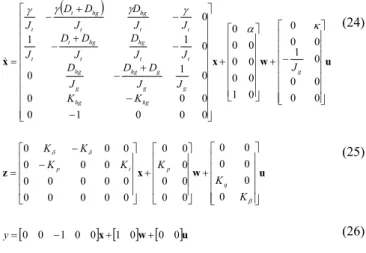
nominal linear model for the WECS. In the nonlinear Cpxλ and Cqxλ
characteristics of a WT for β= 0o, which is shown in Fig. 3, it is
possible to identify two distinct regions in the WT operation. The stall region (A) is characterized by a positive slope, resulting in an unstable operation with sudden and significant drops in the aerodynamic torque. The stable operational region (B) is characterized by a negative slope, corresponding to normal WT operation, where the
aerodynamic torque Qa can be linearized as (Novak et al., 1995;
Rocha et al., 2001; Rocha and Martins Filho, 2003):
β
κ
ω
γ
α
& & && = + +
t
a V
Q (15)
where α is a scaling factor for torque disturbance due to wind
variations V&, γ denotes feedback speed coefficient from the drive
train, and κ represents the pitch control gain. In steady state, V& is
the wind fluctuation ΔV, which can be assumed for design purposes
as a white noise with zero mean (Wasynczuk et al., 1981). Since it is
desirable to operate at maximum Cp, the aerodynamic torque
linearization can be performed in the corresponding λopt, which is
always situated in the normal operation region. Considering
nom V as
the nominal wind speed on the WECS location, the coefficients α, γ,
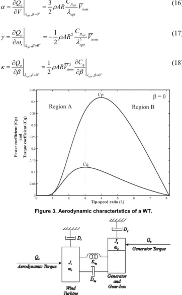
and κ can be easily computed from WT data as:
nom opt p
a ARC V
V
Q opt
o
opt λ
ρ α
β
λ 2
3
0 ,
= ∂
∂ =
=
(16)
nom opt p
t
a AR C V
Q opt
o opt
2 2
0
, 2
1
λ ρ ω
γ
β λ
− = ∂
∂ =
=
(17)
o opt o
opt
q nom
a ARV C
Q
0 , 2
0
, 2
1
=
= ∂
∂ =
∂ ∂ =
β λ β
λ β
ρ β
κ (18)
Figure 3. Aerodynamic characteristics of a WT.
Figure 4. WECS model for control design.
(
t g)
hg mhg a t t tt D Q Q D
J
ω
& +ω
= − −ω
−ω
(19)(
t g)
mhg g hgg g g
g D D Q Q
J
ω
& +ω
=ω
−ω
+ − (20)(
t g)
hg
mhg K
Q& =
ω
−ω
(21)where Jt is the total WT inertia, and Dt= total WT damping.
The linearized equations 15, 19, 20 and 21 constitute the nominal linear state model of a pitch regulated WT. One of the
control inputs is the generator torque Qg, which represents the
electric load mechanically connected to generator. It is adjustable and virtually independent from WECS dynamics (Novak et al.,
1995). The second control input is the pitch angle β, which greatly
impacts the control system due to its active influence on the WT's aerodynamic efficiency. In this context, WECS configures a multivariable system.
Since the dynamics of the pitch actuator is very fast if compared to WT dynamics, it can be considered as an unmodeled uncertainty to avoid an unnecessary increase in the state variables of the nominal model, resulting in a simplest controller with the smallest order. The structural dynamics of the blades and tower are also considered as unmodeled uncertainties in this approach.
Control Objectives
Aiming to explicit the trade-off between the control requirements, the nominal model has to be manipulated using
weighting functions to obtain a generalized system G(s) shown in
Fig. 5, given by:
⎪ ⎩ ⎪ ⎨ ⎧ + + = + + = + + = = u D w D x C y u D w D x C z u B w B Ax x G 22 21 2 12 11 1 2 1 & )
(s (22)
where x = state vector, u = control signals, w = exogenous inputs, z =
control objectives outputs and y = measured outputs. The exogenous
inputs w are signals determined by external processes or environments
that influence the dynamics of the system, such as reference signals, commands, disturbances and noises.
G(s) K(s) w u z y
Figure 5. Generalized system.
The main control requirement of WECS is to reduce detrimental dynamic loads on the shaft, which is obtained by minimization of the shaft torque variations over all bandwidth. In this context, the
first control objective output z1 is obtained by weighting the
difference Δω = ωt - ωg with a fixed gain Kδ. Another important
control requirement for fixed and variable speed WECS is the WT rotation control, which can be defined as the reduction of the
rotation error et= ωsp - ωt. Thus, the second control objective output
z2 is generated by weighting et with a PI function:
s K K s e s z s K i p t
e = = +
) (
) ( )
( 2 (23)
which implies in the augmentation of the original nominal model with an integrator. The control design has to minimize the effects of wind fluctuation and ripple torque over the energy delivered to
electric load, generating the third control objective output z3, which
is obtained by weighting the generator torque Qg with a fixed gain
Kq. Finally, it is necessary to limit the bandwidth of pitch control
input β by weighting it with a fixed gain Kβ. The exogenous inputs
w on WECS are the rotation reference ωsp and wind fluctuation V&.
Due to practical constraints relative to the assembly, cost and
maintenance of the sensors, the generator rotation ωg is considered
the only measured output y. Considering u = [Qgβ]´, w = [ωspV&]´
and x = [QaωtωgQmhg
∫
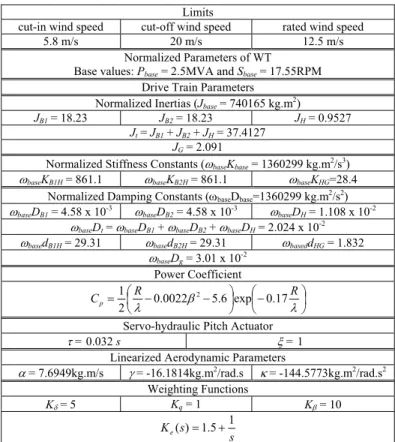
etdt]´, the nominal WECS model augmentedwith weighting functions is given by:
(
)
u w x x ⎥ ⎥ ⎥ ⎥ ⎥ ⎥ ⎥ ⎦ ⎤ ⎢ ⎢ ⎢ ⎢ ⎢ ⎢ ⎢ ⎣ ⎡ − + ⎥ ⎥ ⎥ ⎥ ⎥ ⎥ ⎦ ⎤ ⎢ ⎢ ⎢ ⎢ ⎢ ⎢ ⎣ ⎡ + ⎥ ⎥ ⎥ ⎥ ⎥ ⎥ ⎥ ⎥ ⎥ ⎥ ⎦ ⎤ ⎢ ⎢ ⎢ ⎢ ⎢ ⎢ ⎢ ⎢ ⎢ ⎢ ⎣ ⎡ − − + − − + − − + − = 0 0 0 0 0 1 0 0 0 0 1 0 0 0 0 0 0 0 0 0 0 1 0 0 0 0 0 1 0 0 1 1 0 g hg hg g g g hg g hg t t hg t hg t t t t hg t hg t t J K K J J D D J D J J D J D D J J J D J D DJ α κ
γ γ γ γ & (24) u w x z ⎥ ⎥ ⎥ ⎥ ⎥ ⎦ ⎤ ⎢ ⎢ ⎢ ⎢ ⎢ ⎣ ⎡ + ⎥ ⎥ ⎥ ⎥ ⎦ ⎤ ⎢ ⎢ ⎢ ⎢ ⎣ ⎡ + ⎥ ⎥ ⎥ ⎥ ⎦ ⎤ ⎢ ⎢ ⎢ ⎢ ⎣ ⎡ − − = β δ δ K K K K K K K q p i p 0 0 0 0 0 0 0 0 0 0 0 0 0 0 0 0 0 0 0 0 0 0 0 0 0 0 0 0
0 (25)
[0 0 −1 0 0] [x+1 0] [w+0 0]u
=
y (26)
H2 Methodology
The H2 controller design can be formalized as an optimization
problem, where the goal is to find a controller K2 that internally
stabilizes the system G(s), so that H2 norm:
( ) (
)
[
]
∫
−+∞∞ −= jω H jω dω zw
zw
zw H H
H
2 1 2
(27)
is minimized, where Hzw denotes the transfer function matrix from
exogenous inputs w to objective outputs z. This H2 optimization
problem is equivalent to the conventional LQG problem (Skogestad and Postlethwaite, 2001) involving a cost function:
[
]
dtJ ⎥ ⎦ ⎤ ⎢ ⎣ ⎡ ⎥ ⎦ ⎤ ⎢ ⎣ ⎡ ′ ′ ′ ′ ′ ′ =
∫
∞ u x D D C D D C C C u x 0 12 12 1 12 12 1 11 (28)
with correlated white noises ξ (states) and η (measurements) entering
in the system via w channel associated with the correlation function:
(
τ)
δ τ η τ η τ ξ τ η τ η τ ξ τ ξ τ ξ − ′ ⎥ ⎦ ⎤ ⎢ ⎣ ⎡ ′ ′ ′ ′ = ⎭ ⎬ ⎫ ⎩ ⎨ ⎧ ⎥ ⎦ ⎤ ⎢ ⎣ ⎡ ′ ′ ′ ′ t E 12 12 1 12 12 1 1 1 ) ( ) ( ) ( ) ( ) ( ) ( ) ( ) ( D D B D D B B
B (29)
This problem can be solved by the resolution of the following two Riccatti equations
0 1 1 2 2 2 2 2
2A′+AY −YC′C Y +BB′ =
Y (30)
0 1 1 2 2 2 2 2
2+ − ′ + ′=
′X X A X BB X CC
A (31)
resulting in an H2 optimal controller K2(s) given by:
( )
(
)
⎩ ⎨ ⎧ ′ − = ′ + ′ − ′ − = = x X B u C Y x C C Y X B B A x K ˆ ˆ ˆ 2 2 2 2 2 2 2 2 2 2 2 y sH∞ Methodology
Feedback control design can be also formalized in terms of H∞
norm optimization. The sub-optimal H∞ control problem is to find all
admissible compensators K∞(s) which internally stabilize the
generalized system G(s) and minimize the norm (Doyle et al., 1989):
[ ]
zwzw H
H σ
ω
sup
=
∞ (33)
such that ||Hzw||∞<ε. Considering D11 = 0 and D22 = 0, the solution of
this problem can be given by:
( )
(
)
⎩ ⎨ ⎧
′ − =
+ −
′ − = =
∞
∞ ∞
∞ ∞
∞
x X B u
L x C L X B B A x K
ˆ ˆ ˆ
2 2 2
2 y
s
& (34)
where
∞ − ∞=A+ BB′X
A 1 1
2
ε (35)
(
)
21 2
C Y X Y I
L = − ∞ ′
− ∞ ∞ −
∞ ε (36)
and X∞ and Y∞ are the solutions for two Riccatti equations:
0
1
1 =
′ + ′ − +
′X∞ X∞A X∞B∞B∞X∞ CC
A (37)
0 1
1 ′=
+ ′ − ′
+ ∞ ∞ ∞ ∞ ∞
∞A AY YC C Y BB
Y (38)
where
2 2 1 1 2
B B B B B
B∞ ′∞=ε− ′− ′ (39)
2 2 1 1 2
C C B C C
C∞ ′∞=ε− ′− ′ (40)
The existence of a solution for H∞ control problem is assured by
the following conditions: X∞ ≥ 0, Y∞ ≥ 0 and the eigenvalues
ρ(X∞Y∞) ≤ε2. The best solution for sub-optimal/optimal H∞ controller
can be computed using the loop-shifting two-Riccatti formulae (Chang and Safonov, 1996).
Simulation Results
Plant Description
The WECS considered in this paper consists of an upwind Horizontal Axis WT coupled to a 2.5MW four-pole electric generator by a gear-box (ratio 1:102.5) as shown in Fig. 6 (Wasynczuk et al., 1981). This WT has two blades (NACA230XX series airfoil), each one with a length of 45.72 m, where the outer 30% corresponds to the variable-pitch section controlled by a servo-hydraulic actuator. The generator and other support equipment are enclosed in a nacelle, which is mounted atop a tower with 60.96 m where wind measurements are performed. A yaw control allows the correct alignment of the WT rotor with the wind direction. The complex nonlinear and stochastic mathematical model presented in the section “WECS Model” is used to simulate this WECS, while the nominal model described in the subsection “Nominal Linear Model” is used to design the controllers. The scheme for dynamic simulation for this closed-loop WECS is described in Fig. 7. The main data of this WECS are presented in table 1, including an approach for the power coefficient obtained from the blade
geometry. To compute the parameters of the nominal model, the effective average wind speed is considered as 7m/s.
Figure 7. Block diagram of the dynamic simulation of the WECS control.
Table 1. WECS data.
Limits
cut-in wind speed cut-off wind speed rated wind speed
5.8 m/s 20 m/s 12.5 m/s
Normalized Parameters of WT Base values: Pbase= 2.5MVA and Sbase= 17.55RPM
Drive Train Parameters Normalized Inertias (Jbase= 740165 kg.m2)
JB1= 18.23 JB2= 18.23 JH= 0.9527
Jt= JB1+ JB2+ JH= 37.4127
JG= 2.091
Normalized Stiffness Constants (ωbaseKbase= 1360299 kg.m2/s3)
ωbaseKB1H= 861.1 ωbaseKB2H= 861.1 ωbaseKHG=28.4
Normalized Damping Constants (ωbaseDbase=1360299 kg.m2/s2)
ωbaseDB1= 4.58 x 10⁻³ ωbaseDB2= 4.58 x 10⁻³ ωbaseDH= 1.108 x 10⁻²
ωbaseDt= ωbaseDB1+ωbaseDB2+ ωbaseDH= 2.024 x 10⁻²
ωbasedB1H= 29.31 ωbasedB2H= 29.31 ωbaseddHG= 1.832
ωbaseDg = 3.01 x 10⁻²
Power Coefficient
⎟ ⎠ ⎞ ⎜ ⎝ ⎛− ⎟ ⎠ ⎞ ⎜
⎝
⎛ − −
=
λ β
λ
R R
Cp 0.0022 5.6 exp 0.17 2
1 2
Servo-hydraulic Pitch Actuator
τ = 0.032 s ξ = 1 Linearized Aerodynamic Parameters
α = 7.6949kg.m/s γ= -16.1814kg.m2/rad.s κ = -144.5773kg.m2/rad.s2
Weighting Functions
Kδ = 5 Kq = 1 Kβ= 10
s s Ke( )=1.5+1
The frequency response of the open-loop WECS is shown in Fig. 8. Although high frequency wind fluctuations are well rejected, WECS is very affected by low frequency wind disturbances. It is
noted that the control input β is more effective on WT regulation
than Qg, although it reduces energy conversion efficiency. Torsional
modes can be excited by sudden wind variations and/or operational disturbances since this WECS presents a resonance peak on:
s rad J
J K
g t hg
res 1.9752 /
1 1
= ⎟ ⎟ ⎠ ⎞ ⎜
⎜ ⎝ ⎛
+ =
ω (41)
H2 Controller Performance
Considering the WECS presented in the subsection “Plant
Description”, the use of the H2 design procedure results in the
following controller:
⎥ ⎥ ⎥ ⎥
⎦ ⎤
⎢ ⎢ ⎢ ⎢
⎣ ⎡ =
6 -2
3 4 5
2 3 4
6 -2
3 4 5
2 3 4
2
7.547x10 + 7.454s + 13.27s + 11.09s + 4.504s + s
0.07599 -0.5969s -1.269s -0.6949s -0.2345s
-10 7.547x + 7.454s + 13.27s + 11.09s + 4.504s + s
0.7238 -2.761s -3.923s -0.6462s -0.07592s
)
(s
K
The frequency response of the closed-loop WECS with an H2
controller is shown in Fig. 9. High frequency wind fluctuations are submitted to strong attenuation. For frequencies below 0.7 rad/s, the
sensitivity function (et/ωsp) decays rapidly when the frequency tends
to zero, as shown in its Bode plots, satisfying the requirements related to disturbance rejections. Bode plots of the complementary
sensitivity function (ωg/ ωsp) show that the H2 controller attenuates
measurements noise above 0.7 rad/s, assuring good robustness against uncertainties above this frequency. In regards to the rotation
difference Δω, the excitation of torsional modes is difficult due to an
adequate attenuation of reference variations and/or operational disturbances. Although power fluctuations on the electric load are attenuated, the system's response to variations of the electric torque
Qg will be slow.
The simulation results presented in Fig. 10 show the dynamic behavior of the fixed-speed closed-loop WECS when submitted to a wind gust with duration of 90 s. After this event, both control inputs
are simultaneously used in the rotation regulation, and ωt returns to
its reference value ωsp after approximately 5 minutes. Considering a
variable speed operation, the rotation reference must be adjusted to:
V R
opt sp
λ
ω = (42)
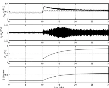
The simulation results presented in Fig. 11 verify the effect of a wind step variation of 7.5 m/s to 9.5 m/s in the dynamic behavior of
the variable-speed closed-loop WECS. In this case, ωt follows speed
reference ωsp, reaching zero error after 10 minutes. Aiming to adjust
ωt, the generator torque Qg is practically duplicated, increasing the
energy delivered to the electric load. Considering that β has a
detrimental effect on energy conversion efficiency, the relatively small contribution of this control input on rotation regulation is positive for variable speed WECS. The system's operation does not excite any torsional modes and the noises introduced by wind
fluctuation are filtered by the H2 controller.
10−2 100 102 −300
−200 −100 0 100
Magnitude
a) From V to ω
t
10−2 100 102 −200
−100 0 100 200
Phase
frequency
10−2 100 102 −300
−200 −100 0 100
b) From Qg to ω
t
10−2 100 102 −200
−100 0 100 200
frequency
10−2 100 102 −300
−200 −100 0 100
c) From β to ω
t
10−2 100 102 −200
−100 0 100 200
10−2 100 102 −250 −200 −150 −100 −50 0 50 Magnitude
d) From V to ∆ω
10−2 100 102 −400 −300 −200 −100 0 100 Phase frequency
10−2 100 102 −250 −200 −150 −100 −50 0 50
e) From Q
g to ∆ω
10−2 100 102 −400 −300 −200 −100 0 100 frequency
10−2 100 102 −250 −200 −150 −100 −50 0 50
f) From β to ∆ω
10−2 100 102 −400 −300 −200 −100 0 100 frequency
Figure 8. Bode plots of linearized open-loop WECS model.
10−2 100 102 −250 −200 −150 −100 −50 0 50 Magnitude
a) From ω
st to ∆ω
10−2 100 102 −500 −400 −300 −200 −100 0 100 200 Phase frequency
10−2 100 102 −250 −200 −150 −100 −50 0 50
b) From ω
st to et
10−2 100 102 −500 −400 −300 −200 −100 0 100 200 frequency
10−2 100 102 −250 −200 −150 −100 −50 0 50
c) From ω
st to Qg
10−2 100 102 −500 −400 −300 −200 −100 0 100 200 frequency
10−2 100 102 −250 −200 −150 −100 −50 0 50
d) From ω
st to ωg
10−2 100 102 −500 −400 −300 −200 −100 0 100 200 frequency
10−2 100 102 −300 −250 −200 −150 −100 −50 0 Magnitude
d) From V to ∆ω
10−2 100 102 −500 −400 −300 −200 −100 0 100 200 Phase frequency
10−2 100 102 −300 −250 −200 −150 −100 −50 0
e) From V to e
t
10−2 100 102 −500 −400 −300 −200 −100 0 100 200 frequency
10−2 100 102 −300 −250 −200 −150 −100 −50 0
f) From V to Q
g
10−2 100 102 −500 −400 −300 −200 −100 0 100 200 frequency
10−2 100 102 −300 −250 −200 −150 −100 −50 0
d) From ω
st to ωg
10−2 100 102 −500 −400 −300 −200 −100 0 100 200 frequency
Figure 9. Bode plots of H2 closed-loop WECS.
0 5 10 15 20 25 30
6 8 10
V (m/s)
time (min)
0 5 10 15 20 25 30
0 0.2 0.4 ωsp , ωt (PU)
0 5 10 15 20 25 30
−0.01 0 0.01 ωt − ωg (PU)
0 5 10 15 20 25 30
2.5 3 3.5
Qg
(PU)
0 5 10 15 20 25 30
0.25 0.3 0.35 β (degree) time (min)
Figure 10. H2 closed-loop WECS at fixed-speed operation: wind gust.
0 5 10 15 20 25 30
0 0.2 0.4 ωsp , ωt (PU)
0 5 10 15 20 25 30
−0.02 0 0.02 ωt − ωg (PU)
0 5 10 15 20 25 30
2 4 6
Qg
(PU)
0 5 10 15 20 25 30
0.5
β
(degree)
time (min)
Figure 11. H2 closed-loop WECS at variable-speed operation: wind step.
H∞ Controller Performance
Considering the WECS presented in the subsection “Plant
Description”, the optimal H∞ controller is obtained with ε= 0.0674:
⎥ ⎥ ⎥ ⎥ ⎦ ⎤ ⎢ ⎢ ⎢ ⎢ ⎣ ⎡ = ∞ 5 -2 3 4 5 2 3 4 5 -2 3 4 5 2 3 4 10 5.18x + 51.75s + 92.42s + 52.89s + 16.25s + s 0.22 -2.58s -6.059s -3.18s -1.138s -10 5.18x + 51.75s + 92.42s + 52.89s + s 16.25 + s 0.3474 -2.685s -s 8.93 -s 2.253 -2.297s ) (s K
The frequency response of closed-loop WECS with the H∞
controller is shown in Fig. 12. Notice that high frequency wind fluctuations are strongly attenuated. The sensitivity function decays rapidly for frequencies below 0.7 rad/s and the complementary sensitivity function is attenuated above 0.7 rad/s, assuring the requirements related to disturbance rejections and robustness against
uncertainties. The H∞ controller provides adequate attenuation of the
reference variations or operational disturbances and, if compared to
the H2 controller, it provides a greatest attenuation for power
fluctuations in the grid, resulting in an extremely slow response for
variations on electric torque Qg.
In relation to a fixed-speed operation, the dynamic behavior of
duration of 180 s is shown in Fig. 13. If compared with the H2
controller, this controller presents better robustness, without unstable behavior when submitted to greatest disturbances. The control system is able to reject the effects of this wind disturbance
using simultaneously β and Qg. The turbine speed ωt returns to its
reference value ωsp approximately at the end of the wind gust. The
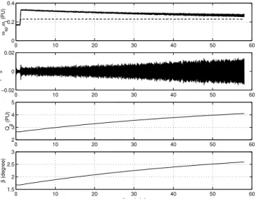
simulation results for variable speed closed-loop WECS when submitted to wind step variation from 7.5 m/s to 9.5m/s are shown
in Fig. 14. Notice that the β performance on the rotation adjustment
is improved. Although ωt will eventually reach the reference ωsp,
this adjustment is extremely slow.
Conclusions
H2 or H∞ optimal feedback control problem involves finding a
controller K for a generalized system G(s), using optimization
techniques for the respective norms. Although both approaches
present several similarities, the H∞ methodology results in a more
conservative controller than the H2 methodology, since the
disturbance signal dependency is considered in the H∞ controller
design. Thus, the H∞ controller presents a better robustness than a
similar H2 controller, but its dynamic response is extremely slow.
Although the H∞ solution can be relatively flexible, admitting
sub-optimal controllers, the tendency is to use the H∞ controller in
applications involving regulation problems, such as fixed-speed closed-loop WECS, where the output has to stay at determined value despite the presence of great disturbances. In counterpart, the fast
response of the H2 controller is more adequate for applications
involving tracking problems, such as variable-speed closed-loop WECS, since it is necessary to follow a reference imposed by the wind speed to obtain maximum energy conversion. In this context, an interesting option for WECS controller designs can be the
multi-objective H2/H∞ optimal control approach, where several channels
associated with different norms are established, aiming to simultaneously attend several performance criteria.
10−2 100 102 −250
−200 −150 −100 −50 0
Magnitude
a) From ω
st to ∆ω
10−2 100 102 −800
−600 −400 −200 0 200
Phase
frequency
10−2 100 102 −250
−200 −150 −100 −50 0
b) From ω
st to et
10−2 100 102 −800
−600 −400 −200 0 200
frequency
10−2 100 102 −250
−200 −150 −100 −50 0
c) From ω
st to Qg
10−2 100 102 −800
−600 −400 −200 0 200
frequency
10−2 100 102 −250
−200 −150 −100 −50 0
d) From ω
st to ωg
10−2 100 102 −800
−600 −400 −200 0 200
frequency
10−2 100 102 −400
−300 −200 −100 0
Magnitude
d) From V to ∆ω
10−2 100 102 −600
−400 −200 0 200
Phase
frequency
10−2 100 102 −400
−300 −200 −100 0
e) From V to e
t
10−2 100 102 −600
−400 −200 0 200
frequency
10−2 100 102 −400
−300 −200 −100 0
f) From V to Q
g
10−2 100 102 −600
−400 −200 0 200
frequency
10−2 100 102 −400
−300 −200 −100 0
d) From ω
st to ωg
10−2 100 102 −600
−400 −200 0 200
frequency
Figure 12. Bode plots of H∞ closed-loop WECS.
0 5 10 15 20 25 30
6 8 10
V (m/s)
0 5 10 15 20 25 30
0 0.2 0.4
ωsp
,
ωt
(PU)
0 5 10 15 20 25 30
−0.01 0 0.01
ωt
−
ωg
(PU)
0 5 10 15 20 25 30
2.4 2.6 2.8
Qg
(PU)
0 5 10 15 20 25 30
1.5 1.6 1.7
β
(degree)
time (min)
Figure 13. H∞ closed-loop WECS at fixed-speed operation: wind gust.
0 10 20 30 40 50 60
0 0.2 0.4
ωsp
,
ωt
(PU)
0 10 20 30 40 50 60
−0.02 0 0.02
ωt
−
ωg
(PU)
0 10 20 30 40 50 60
2 3 4 5
Qg
(PU)
0 10 20 30 40 50 60
1.5 2 2.5 3
β
(degree)
time (min)
References
Anderson, P.M. and Bose, A., 1983, “Stability simulation of wind turbine systems”, IEEE Trans. on Power Apparatus and Systems, Vol. 102, No. 12, pp. 3791-3795.
Chang, R.Y., and Safonov M.G., 1996, “Robust control toolbox for use with matlab”, Mathworks Inc., USA.
Dessaint, L., Nakra, H., and Mukhedkar, D., 1986, “Propagation and elimination of torque ripple in a wind energy conversion system”, IEEE Trans. on Energy Conversion, Vol. 1, No. 2, pp. 104-112.
Doyle, J.C., Glover, K., Khargonekar, P.P., and Francis, B.A., 1989, “State-space solutions to standart H2 and H∞ control problems”, IEEE Trans. on Automatic Control, Vol. 34, No. 8, pp. 831-846.
Freris, LL., 1990, “Wind Energy Conversion Systems”, Prentice Hall Inc., United King.
Golding, E.W., 1977, “The Generation of Electricity by Wind Power”, E. & F. N. Spon LTD, United King.
Hori, Y., Sawada, H., and Chun, Y., 1999, “Slow resonance ratio control for vibration suppression and disturbance rejection in torsional system”,
IEEE Trans. on Industrial Electronics, Vol. 46, No. 1, pp. 162-168. Hwang, H.H., and Gilbert, L.J., 1978, “Synchronization of wind turbine generators against an infinite bus under gusting wind conditions”, IEEE Trans. on Power Apparatus and Systems, Vol. 97, No. 2, pp. 536-544.
Johnson, C.C. and, Smith R.T., 1976, “Dynamics of wind generators on eletric utility networks”, IEEE Trans. on Aerospace and Eletronics Systems, Vol. 12, No. 4, pp. 483-493.
Lefevbre, S. and, Dubé, B., 1988, “Control system analysis and design for an aerogenerator with eigenvalue methods”, IEEE Trans. on Power Systems, Vol. 3, No. 4, pp. 1600-1608.
Leith, D.J., and Leithead, W., 1997, “Implementation of wind turbine controllers”, International Journal of Control, Vol. 66, No. 3, pp. 349-380.
Leithead, W.E., de la Salle, S., and Reardon, D., 1991, “Role and objectives of control for wind turbines”, IEE proceedings-C, Vol. 138, No. 2, pp. 135-148.
Maciejowski, J.M., 1989, “Multivariable Feedback Design”, Addison-Wesley Publishing Company Inc., England.
Medeiros, A., Simões, F.J., Lima, A.M.N., and Jacobina, C.B., 1996, “Modelagem aerodinâmica de turbinas eólicas de passo variável”, Proceeding od VI ENCIT / VI LATCYM, ABCM. Florianópolis, Brazil, pp. 25-30.
Novak, P., Ekelund, T., Jovik, I., and Schmidtbauer, B., 1995, “Modeling and control of variable speed wind-turbine drive-system dynamics”, IEEE Control Systems, Vol. 15, No. 4, pp. 28-38.
Raina, G., and Malik, O.P., 1985, “Variable speed wind energy conversion using synchronous machine”, IEEE Trans. on Aerospace and Electronic Systems, Vol. 21, No. 1, pp. 100-104.
Rocha, R., and Martins Filho, L.S., 2003, “A multivariable H∞
control for wind energy conversion system”, Proceedins of IEEE Conference on Control Applications, Istambul, Turkey.
Rocha, R., Resende, P., Silvino, J.L., and Bortolus, M.V., 2001, “Control of stall regulated wind turbine through H∞ loop shaping
methods”, Proceedings of IEEE Conference on Control Applications, Mexico City, Mexico.
Rohatgi, J., and Pereira, A., 1996, “Modeling wind turbulence for the design of large wind turbines – a preliminary analysis”, Proceedings of IV CEM-NNE, pp. 735-739.
Skogestad, A., and Postlethwaite, I., 2001, “Multivariable Feedback Control – Analysis and Design”, John Wiley and Sons.