COMPARISON OF THE LQG AND H-INFINITY TECHNIQUES TO DESIGN
EXPERIMENTALLY A FLEXIBLE SATELLITE ATTITUDE CONTROL SYSTEM
J. V. C. de Castro
University of Minas Gerais, Mechanical Engineering Department Rua Espírito Santos, 35, Belo Horizonte, MG, Brasil.
email: [email protected]
L. C. G. de Souza
National Institute for Space Research, Space Mechanics and Control Division Av. dos Astronautas, 1758, S J dos Campos, SP, Brasil
email: [email protected] or [email protected]
Abstract: Attitude Control System (ACS) for flexible space satellites demands great reliability, autonomy and robustness. These flexible structures face low stiffness due to minimal mass weight requirements. Satellite ACS design usually based on computer simulations without experimental verification can face instability and/or inefficient controller performance due to model uncertainties. In this paper one investigates the robustness and performance of the time domain approach LQG (Lineal Quadratic Gaussian) and the frequency domain H– Infinity approach. The satellite ACS design is performed initially in a computer simulation environment, following experimentally verification of the same control algorithm, using Quanser rotary flexible link module. This investigation has shown that the controller performance based on simulation model can be degraded when applied in an experimental set up. So this prototype verification is fundamental before satellite onboard computer algorithms implementation.
1 Introduction
also, the CIPID controller performance was compared to a simple proportional controller. In Souza (1996) it was showed that the influence of the non-linearities introduced by the panel’s flexibility and the system parameters variation can degrade the control system performance, indicating the necessity of new robust control technique. In this paper one investigates and compare experimentally the robustness and performance of two different multivariable methodologies in designing the ACS for a rigid-flexible satellite, using Quanser rotary flexible link module. The first one is the traditional time domain approach LQG (Lineal Quadratic Gaussian) and the second one is the frequency domain H–Infinity approach Skogestad and Postlethwaite (2005). This preliminary investigation has shown that the controller performance based on the simulation model can be degraded when applied in an experimental setup Conti and Souza (2008). Besides, these results have shown that the H-infinity controller has the disadvantages of having superior order than the plant, although it can be robust against uncertainties like the nonlinearties of the model Gonzales and Souza (2009), since it takes into account all sources of uncertainties in the controller design.
2 Rigid flexible satellite model
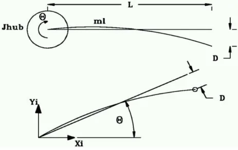
The satellite model consists of a central rigid part clamped to a thin flexible link and the output is an analog signal proportional to the deflection of the link. The experimental set up used is the Quanser rotary servo plant resulting in a horizontally rotating flexible link to perform rigid flexible control. This system is similar in nature to the control problems encountered in large light space structures where the weight constraints result in flexible structures that must be controlled using feedback techniques. A DC motor rotates the flexible link from one end in the horizontal plane. The motor of the link is instrumented with a strain gage that can detect the deflection of the tip. Fig. 1 shows the flexible link at a given rotation angle resulting in the arm end-point displacement D with the flexible link deflection = D/L. Table 1 shows the list of parameters and variables used in the derivation of the state-space equations of the system.
Figure 1. Flexible Link with the rigid rotation and flexible deflection
Table1. Parameters and variables used in the derivation of the system equations of motions
Symbol Description
Length of flexible Link Mass of flexible Link
Strain Gage Calibration factor Servo load gear angle (radians) Arm Deflection (radians) Link End-point Deflection
Link Damped Natural Frequency Link Moment of inertia
3 Equations of motions
Considering a simple mass spring model for the flexible link, the rotary spring equations of motion is given by
J
LINK
K
STIFF
(1)where Kstiff is the link stiffness that is related to flexible link deflection and the link’s damped natural frequency by
c2
(2)Combining equations (1) and (1), one obtains
K
STIFF cJ
LINK2
(3)The system equations of motion are obtained using Lagrange formulation Souza (1996), from the Kinetic and Potential energies of the system. As a result, the Lagrangian function given by
2 2 2 2 22
LINK STIFF
eq J K
J V T
L
(4)
Applying the Lagrange formulation for the generalized coordinates and one obtains the two equations of motions
J
eq
J
ARM
T
OUTPUT
B
eq
(5)
J
ARM
K
STIFF
0
(6)where the output torque on the load from the motor is given by
m m g m g T g m OUTPUT
R
K
K
V
K
K
T
)
(
(7)Combining equations (5), (6) and (7), one obtains the complete system state-space equations of motion given by
m m eq g T g m m eq g T g m m eq m eq g m T g m ARM eq ARM eq STIFF m eq m eq g m T g m eq STIFFV
R
J
K
K
R
J
K
K
R
J
R
B
K
K
K
J
J
J
J
K
R
J
R
B
K
K
K
J
K
0
0
0
0
0
0
1
0
0
0
0
1
0
0
2 2
(8)Where m and g are the motor and gearbox efficiencies, KT and Kg are transmission and motor rate. Rm is the armature resistance,Vm the armature input voltage, Km the back-emf constant and Jeq theequivalent moment of inertia at the load. Details of this derivation can be found in Quanser Manual Quanser homepage.
4 The LQG method
Considers the state estimation problem of a stochastic system given by
where w (t) and v (t) are Gaussian noises with mean zero and having covariance’s
E
w
(
t
)
w
'
(
t
)
W
0
,E
v(t)v'(t)
V 0,E
w
(
t
)
v
'
(
t
)
0
(10)The input u(t) represents the control vector, y(t) the vector of measured outputs, w (t) and v (t) are the system and measures noise, respectively.
The solution of the LQG problem consists in obtained a feedback control law that minimizes the cost
0
dt
))
t
(
Ru
)
t
(
'
u
)
t
(
Qx
)
t
(
'
x
(
E
lim
J
(11)By the separation principle, the solution of the LQG problem reduces to two sub-problem Souza (1996). The first one is the LQR problem which aims at to design an optimal control law u, such that, minimizes the deterministic cost given by
0
dt )) t ( Ru ) t ( ' u ) t ( Qx ) t ( ' x (
J (12)
where the matrices Q and R are semi-positive and positive defined, respectively. The system is represented by
x
(
t
)
Ax
(
t
)
Bu
(
t
)
(13)and the control law is defined by
u
K
r(
t
)
x
(
t
)
(14)with the gain K(t) is given by
Kr R1B'P(t) (15)
and P(t) is the solution of Riccati equation
P
A
'
P
PA
Q
PBR
1B
'
P
(16)In the stationary case, the Riccati equation is equal to zero. The LQR approach assumes that the system dynamic is perfect, there are no disturbances, and all states are available to feedback, a hypothesis that does not occur in the majority of the application.
The second one is the Kalman Filter problem given by a state estimator of the form
x
ˆ
(
t
)
(
A
K
fC
)
x
ˆ
(
t
)
Bu
(
t
)
K
fy
(17)with the control law u = -Kr
x
ˆ
based on the estate estimated vectorsx
ˆ
, and the Kalman filter gain is given by
K
F
P
KC
TV
1 (18)where PK satisfies another algebraic Riccati equation
0APKPKA'GWG'PKC'V1CPK (19)
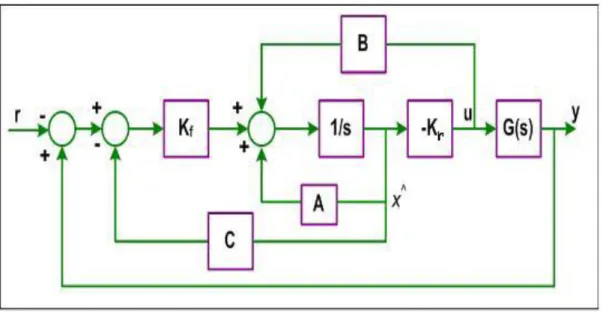
Figure 2. Series connection of the LQG Controller Structure
5 The H-infinity method
The H∞ control theory Skogestad and Postlethwaite (2005) combines concepts of the time and frequency domain in order to give a unified solution. Its advantage is the ability to include in the solution of optimization problem requirements of performance as bandwidth, time of response and minimization of the cost function. Fig. 3, shows a general configuration of the H∞ method, where the signal w represents the entries outside the system, z is the signal error, composed of all those signals needed to characterize the behavior of the closed loop system, u is the sign of control, and e is the sign of difference between the exit y and entries w. The problem of control is to determine a gain K that stabilize the plant G and minimize the transfer functions between w and z.
Figure 3. General Configuration of H∞ method
The H∞ controller is base on the state space system
Du
Cx
y
Bu
Ax
x
(20)
which in more details is given by
) (
) (
) (
.
) (
) (
) (
22 21 2
12 11 1
2 1 .
t u
t w
t x
D D C
D D C
B B A
t y
t z
t x
Figure 4 shows that the plant is formed with the weight W1, W2 and W3. In the design controller good performance and robustness are function of the weight, so as, z1 = W1e; z2 = W2y and z3 = W3u.
Figure 4. Augmented plant with the weight used in the H∞ controller design
In the H-infinity controller design the central tuning parameter is the mixed sensibility function given by
1 1 1
3 2 1
1 1
)
(
)
(
)
(
GK
I
GK
T
GK
I
K
R
GK
I
S
T
W
R
W
S
W
N
yu (22)where S is the sensibility function, T complementary sensibility function and R is the energy function. The mixed sensibility function has the property of penalizing at the same time S, R and T, which are treated as project requirements. From Fig. 5 one observes that transfer function from w to z1 is the sensitivity function W1S, associated to the performance of tracking putting a lower limit on the bandwidth of the closed loop system. The transfer function from w to z2 is the function W2 R, associated to the control energy and the transfer function from w to z3 is the function W3T, which minimize low gains at high frequencies.
6 Simulation and experimental results
Figure 5. Complete Quanser flexible link set up used to run real time algorithms
The Hoo controller poor performance can be associated to the no modelled dynamics of the plant, since this source of uncertainty was not considered in the computer controller design. In the experimental apparatus there is a lot of this kind of uncertainty, due to the wire connections. This behaves also shows that the Hoo controller is more sensitive than LQR and LQG controllers. However, as for energy limit, fig. 7 shows that the Hoo controller has superior experimental performance than the LQR and LQG controller, since the LQR and LQG peaks are greater than the Hoo controller. Finally, it is important to say that the three controllers are function of they tuning weight matrices, which once better designed will improve these controller performances.
Figure 7. Controllers’ performance in terns of energy limits
The performance difference between the computer controller design and experimentally implementation was also associated to the integration time. Because, in computer simulation design the integration algorithms were better and more precise, with the possibility of using variable time steps, while in the experimental implementation the time steps were restrict to the sample time of 1 Khz for construction reasons. Another problem that could affect the controller performance was that the Hoo controller gain (KHoo) was a transfer function of high order, consequently, demanding more process time than the LQR and LQG controller, since the gains of both were constant matrix.
7 Summary and conclusions
8 References
B., A., Albassam, Fast maneuver control design for flexible structures using concentrated masses.
Journal of Sound and Vibration,
273, (2004), 755-775.
C., D., Hall, P., Tsiotras, H., Shen., Tracking Rigid Body Motion Using Thrusters and Momentum Wheels, Journal of the Astronautical Sciences, 2002.
D., Dichmann, J., Sedlak, Test of a Flexible Spacecraft Dynamics Simulator. Published by AAS in Advances in
the Astronautical Sciences, 100, I, (1998), 501-526. Paper AAS 98-340.E., G., Barbosa, L., C., S., Góes, Flexible structure control and validation using Flexgage Quanser
system. In ABCM. 19th International Congress of Mechanical Engineering.
Brasília, DF, Brasil,
2007.
G., T., Conti, L., C., G., Souza, Satellite attitude control system simulator. Journal of Sound and
vibration. 15, 3-4, (2008), 395-402.
G., T., F, Conti, Satellite Attitude Control System Simulator. Proceedings of the National Institute for Space Research Seminar – SICINPE, August, Brasil, 2006.
J., L.,
Schwartz, M., A., Peck, C., D., Hall, Historical review of air-bearing spacecraft simulators.
Journal of Guidance, Control and Dynamics
,
26, 4, (2003),513-522.
J., Prado, G., Bisiacchi, L., Reyes, E., Vicente, F., Contreres, M., Mesinas, A., Juares, Three-axis
air-bearing based platform for small satellite attitude determination and control simulation. Journal of
Applied Research and Technology, 3, 3, (2005), 222-237.
L., C., G., Souza, Dynamics and Robust Control for Uncertain Flexible Space System, PhD Thesis, Cranfield Institute of Technology, CoA, Cranfield, England, 1992.
L., C., G., Souza, Robust controllers design for flexible space system using a combination of
LQG/LTR and PRLQG methods. In: Dynamics and Control of Structure in Space III. U.K.: C. L.
Kirk and D. J. Inman, (1996), 151-166.
M., H., Kaplam, Modern Spacecraft Dynamics and Control, John Wiley & Sons New Your, 1976.
M., M., Berry, B., J., Naasz, H., Y., Kim, C., D., Hall, Integrated Orbit and Attitude Control for a Nano Satellite with Power Constrains. AAS/AIAA Space Flight Mechanical Conference. P. Rico, February, 9-12, 2003. O., Holub, Development for VLT Telescope Controller Design
.
PhD thesis, Katedra Rídicí Techniky,
2005.
P., Tsiotras et al, A Spacecraft Simulator for Research and Education. Paper of Georgia Institute of Technology, EUA, 2007.
Quanser homepage. At: <http://www.quanser.com/>.
R., G., Gonzales, L., C., G., Souza, Application of the SDRE method to design a control system
simulator. Advances in Astronautical Sciences. 134, (2009), 2251-2258.
R., H., Cannon, D., E., Rosenthal, Experiments in control of flexible structures with noncolocated sensors and actuators. Journal of Guidance. AIAA, 7 ,5 , (1984), 546-553.