J. Braz. Comp. Soc. vol.14 número4

NP-complete. There are many approaches for the CLSP with a single item, with multiple items and with only one or multiple production centers. Usually these problems are tackled heuristically [24, 12, 5], though exact solution methods exist to solve them [4], [19] and [2].

The multi-plant capacitated lot sizing problem (MPCLSP) with multiple items and periods is composed of multiple production centers that produce all the same items as well as enabling transfers amongst the plants. Sambasivan and Schimidt [17] solved this problem with a heuristic based on transfers of production lots between the periods and the plants, while even better results were ob-tained by Sambasivan and Yahya [18] using a Lagrangian relaxation. Nevertheless, Nascimento et al. [14] intro-duced a GRASP (Greedy Randomized Adaptive Search Procedures) heuristic as well as a path relinking intensifica-tion procedure that outperformed the heuristic proposed in [18].

There have been few studies on MPCLSP and no ap-proach with setup carry-over was presented until now. The problem with setup carry-over considers two additional possibilities: to conserve the setup for one item along two consecutive periods, i.e., the setup carry-over occurs when the last item of a certain period is the first item to be pro-duced in the next period; to allow using the idle capacity in one period in order to make the setup of the first item to be produced in the next period. Besides reducing setup cost, this strategy provides additional capacity with the lack of setup time between consecutive periods. As can be observed, it is necessary to judge which items are the first

Abstract

This paper addresses the capacitated lot sizing problem (CLSP) with a single stage composed of multiple plants, items and periods with setup carry-over among the periods. The CLSP is well studied and many heuristics have been proposed to solve it. Nevertheless, few researches explored the multi-plant capacitated lot sizing problem (MPCLSP), which means that few solution methods were proposed to solve it. Furthermore, to our knowledge, no study of the MPCLSP with setup carry-over was found in the literature. This paper presents a mathematical model and a GRASP (Greedy Randomized Adaptive Search Procedure) with path relinking to the MPCLSP with setup carry-over. This solution method is an extension and adaptation of a previously adopted methodology without the setup carry-over. Computational tests showed that the improvement of the setup carry-over is significant in terms of the solution value with a low increase in computational time.

Keywords: GRASP, path relinking, lot sizing, multiplant, carry-over.

1. I

The capacitated lot sizing problem (CLSP) is a tacti-cal production problem which consists in deciding when and how many items to produce minimizing the produc-tion costs assuring the demand constraints. According to Maes et al. [13] the decision problem to determine if there is a feasible solution to the CLSP with setup time is

Multi-Plant Capacitated Lot Sizing

Problem With Setup Carry-Over

Mariá C. V. Nascimento and Franklina M. B. Toledo

Instituto de Ciências Matemáticas e de Computação, Universidade de São Paulo – USP,

Av. Trabalhador São-carlense, 400, Centro Phone: +55 (16) 3373-8632, Fax: +55 (16) 3373-9700

C.P. 668, CEP 13560-970, São Carlos - SP, Brazil {mariah | fran}@icmc.usp.br

and the last to be produced along the periods. In addition to this, it is important to know what is the setup state of the machine at the end of a period, i.e., what item is that the machine is ready to produce. The setup carry-over has had widespread success in the single-plant lot sizing prob-lem as can be seen in [10, 20, 9, 16, 21, 3].

This paper presents a mathematical model and a GRASP heuristic embedded with a path relinking strat-egy to approximately solve the MPCLSP with multiple items and multiple periods. The solution method is an extension of previous research of Nascimento et al. [14] on the same problem without the setup carry-over. To treat the setup carry-over we modified the local search of the GRASP heuristic adding some moves in its neighbor-hood. The moves used were based on a modified version of the approach of Gopalakrishnan et al. [9] to consider the various plants. In order to test and evaluate the ef-ficiency of the proposed heuristic with setup carry-over considering a single plant, we compared it with the single-plant tabu search heuristic proposed by Gopalakrishnan et al. [9]. For such, we applied our heuristic to the single-plant instances from [24], i.e., the same set of instances used by Gopalakrishnan et al. [9] in their tests. We also compared the solutions of the heuristic without setup carry-over with the solutions of the Lagrangian heuristic proposed by Trigeiro et al. [24]. Regarding the multi-plant experiment, tests were performed using the data set pro-posed in [14], that is based on the instances from [23] for the CLSP with parallel machines. Computational tests indicate that the setup carry-over showed good perform-ance for both the single-plant and the multi-plant prob-lems with a slight increase of computational time in the latter case. Moreover, in both cases the strategy achieved better solutions for all instances.

The remainder of this paper is organized as follows. Section 2 provides a mathematical model for the MPCLSP with setup carry-over. Section 3 presents the solution ap-proach while Section 4 shows the computational tests and its results. Finally, Section 5 concludes the paper with some remarks and future research directions.

2. M

F

Follows the proposed representation of the MPCLSP in a mathematical model relating the carry-over con-straints. This formulation was inspired by the multiplant model presented in [17] without setup carry-over and by the capacitated lot sizing model presented in [16] for problems with setup carry-over.

, [

( )]

i NI j MI t TI ijt ijt ijt ijt

k MI k j

ijt ijt ijkt ijkt

min c x s y

h I r w

Subject to: 1

,

,

=

ijt ijt ijkt

k MI k j

iljt ijt ijt

l MI l j

I x w

w I d i, j, t (1)

=

( T )( )

ijt ijl ijt ijt

j MI l t

x d y u i, j, t (2)

( _{ijt ijt ijt ijt}) _jt

i NI

b x f y C _{j, t (3)}

1 ijt i NI

u _{j, t (4)}

, 1 , 1

ijt ij t ij t

u y u i, j, t (5)

, 1 , 1

1

ijt ij t kj t

u

y

y

0= 0

ij

I i, j (7)

1= 0

ij

u i, j (8)

, 0

ijt ijt

x I i, j, t (9)

0 ijkt

w i, j, k, t (10)

, {0,1} ijt ijt

y u i, j, t (11)

Indexes

T is the number of periods in the planning horizon; N is the number of items in the planning horizon; M is the number of plants in the planning horizon; TI is the set composed of the elements 1,...,T ; NIis the set composed of the elements 1,...,N; MI is the set composed of the elements 1,...,M;

Data

d_ijt is the demand of item i at plant j in period t;

C_jtis the available capacity of production at plant j in period t; b_ijt is the time to produce a unit of item i at plant j in period t; f_ijt is the setup time to produce item i at plant j in period t; c_ijt is the unit production cost of item i at plant j in period t; s_ijt is the setup cost of item i at plant j in period t;

h_ijt is the unit inventory cost of item i at plant j in period t; r_ijkt is the unit minimum transfer cost of item i from plant j to k in period t;

Variables

x_ijt is the quantity of item i produced at plant j in period t; I_ijt is the quantity of item i stored at plant j at the end of period t; w_ijkt is the quantity of item i transferred from plant j to plant k in period t;

y_ijt is a binary variable that assumes value 1 if there is setup of item i at plant j in period t, and 0, otherwise;

The objective function aims to minimize the produc-tion, setup, inventory and transfer costs, subject to the problem constraints. Constraints (1) ensure that the

de-mand dd_ijtt is satisfied by production at plant jj in period

t or by inventory from the previous period in the same

t

demanded plant or by production transfers from another

plants. Constraints (2) ensure that if x_ijtt is positive, one

of y_ijt andu_ijtt variables assumes the value 1, i.e., there is

no setup to the production in period tt only if the setup

carry-over from the previous period occurs. Furthermore, constraints (3) restrict the capacity of each plant and each period, while the constraints (4) limit to one the number of setup carry-over for each period and plant. Constraints

(5) forceu_ijt= 0 if both there was not setup of item ii in

periodtt – 1 at plant jj y ((

ij,t-1 = 0) and the setup of item iwas

not carry-over in this plant from period tt – 2 (u_ij,t-1= 0).

Constraints (6) allow a setup carry-over of itemii in period

t at plant

t j, i.e,u_ijtt = 1, only if there was setup of such item in

the previous period ((y_ij,t-1 =1) or the plant did not produce

any item different than ii in the previous period and the

setup carry-over came from periodtt – 2 (((y_kj,t-1= 0 kand

u_ij,t-1 = 1).

Constraints (7) and (8) assume, respectively, null ini-tial inventory and no iniini-tial setup carry-over to period 1,

while the constraints (9) and (10) ensure that x_ijt,II_ijt and

w_ijktt variables of the problem are all positives. Finally, the

constraints (11) assume that y

ijt anduijt and zijt are

bina-ries.

3. S

M

In this paper, we propose a GRASP heuristic designed to deal with the requirements and constraints of the mathematical model of Section 2. GRASP is a semi-greedy metaheuristic proposed in [7] and [15]. It is a two phase metaheuristic in which the first one consists of the semi-greedy constructive phase and the second one is the local search. For each solution built in the constructive phase, is applied the local search. In the proposed GRASP, a path relinking intensification strategy was incorporated. Many researchers have exploited GRASP and its hybridization with path relinking ([11]).

Path relinking is a metaheuristic proposed in [8] which looks for a better solution in the path between two solutions, the initial solution and guide solution. The goal is better explores the search space. The basic idea behind our solution method is to find the initial solutions as in [14], and then to apply the local search in each one of them. If the resulting solution is not feasible, then a fea-sibility phase is applied to it. In case that the resulting so-lution of this feasibility phase is feasible, it will pass by

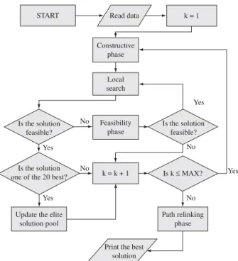
the local search procedure in order to improve its quality. During the GRASP, a pool with the best solutions is kept. After GRASP to be finished, the path relinking phase is performed. The GRASP with path relinking proposed in this paper consists of the flow chart presented in Figure 1. Let MAX be the number of the initial solutions generated by GRASP constructive phase.

The description of the proposed solution method does not use the carry-over variables of Section 2.

3.1. I

S

We obtain an initial solution for the problem by re-laxing the capacity constraints (3) and setup carry-over constraints (4)-(6). It is easy to see that the relaxed

pro-blem can be decomposed inton independent

uncapacita-ted lot sizing with multi-plant subproblems one for each

item i. If we sum up the demands of all plants for each

period (d’_it= ÓM

j=1 ddijt), this problem can be viewed as its

uncapacitated lot sizing problem with parallel machines, jj j

which consists of minimizing a concave function over a convex set (see [22]). It is well known that the minimum occurs in a extreme point that, in the case of a polyhedral

set, has at most the number of constraints (TTT) nonzero

variables. If d’d_itt > 0, then eitherII_ijt > 0 orx_ijt > 0 for some

j 1, ...,MMM}. Thus, every extreme point must satisfy the j j

following property:

I_ij,t-1

I x_ijt = 0 jj = 1...M tMM,t = 1...TTT. (12)

START k = 1

Constructive phase

Local search

k = k + 1 Feasibility

phase Read data

Is the solution feasible? Is the solution

feasible?

Is the solution

one of the 20 best? Is k฀ ฀MAX?

Update the elite solution pool

Path relinking phase

Print the best solution

Yes

Yes Yes

Yes

No

No

No

No

This property is a generalization of the single machine system studied by Wagner and Whitin [26] (see also [1], [6] and [25]). This subproblem can be solved by the dy-namic programming algorithm proposed in [22] using the following recursive equation:

0 < 1

{ } for = 1, , ,

min =

for = 0

ik ijkt

k t j M it

t T

t

0 (13)

where

' , 1 , 1

= 1 1

'

= 1 = 1 =

t

ijkt ij k ij k ir

r k

t t

ijl ir

l k r l

s c d

h d (14)

To solve these subproblems, as in [14], we used a semi-greedy adopted version of the dynamic programming forward recursion (13) as described in Procedure 1. The initial solution is obtained by applying Procedure 1 for all items using a parameter ฀ [0, 1] adopting the same idea to find initial solutions of the original GRASP.

For the resulting initial solution we set the setup carry-over parameters as described in Procedure 2. These parameter settings are different from Gopalakrishnan et al. [9]. We also tested their initial parameter settings, however the proposed strategy performed better. In Procedure 2,a_jt and b_jt denote, respectively, the first and last items pro-duced in period t at plant j. Let e_jt be the state of the ma-chine in the end of period t at plant j.

Most of the initial solutions are infeasible because of the unrestricted capacity of the procedure. To evalu-ate the solution in this case, the total overtime is multi-plied by a penalty which is added to the solution value. The local search performs a search for a feasible and good solution in the neighborhood of the solution found.

3.2. L

S

P

After the seed solution has been constructed, it is improved with the local search. In this paper, the local search has a different structure from the one presented in [14] because here the carry-over moves were added to its neighborhood. In the following, we describe all the moves which compose the neighborhood of the local search procedure. These moves are based on the study of Gopalakrishnan et al. [9] extended here to multiple plants.

Procedure 1 Initial Solution (i฀ ) 1: Calculate d’_it, for t = 1...T ; _i0 = 0

2: fort =1,...,Tdo

3: _Calculate

ijkt for t =1...T , k = 0...t – 1 and j = 1...M; 4: Let S be composed by the elements s with the values

g(s) ฀{

ik + ijkt}, where k = 0...t – 1 and j =1...M;

5: gmin min {g(s)};

s S

6: gmax max {g(s)};

s S

7: Build the RCL (restricted candidate list) using the elements of S such that

g(s) [gmin,gmin+ (gmax–gmin)] with s S;

8: Choose randomly one element s RCL and

let

it g(s); 9: end for

10: Set the transfer variables;

Procedure 2 Initial Carry-over parameters(Sol)

1: Initiate the carry-over parameters a,b and e with zero;

2: forj = 1...M and t = 1...T – 1 do

3: _{S {i|i NI and y}

ijt = yij,t+ 1 = 1};

4: ifS Øthen

5: _b

jt,ejt,aj,t+1 min{i|i S}; 6: end if

7: end for

8: for t = 1...Tdo

9: _ifb

jt = 0 then

10: _b

jt,ejt min {i|yijt = 1 and ajt i}; 1 ฀i฀ ฀N

11: end if

12: _ifa

jt = 0 then

13: _a

jt min {i|yijt = 1 and bjt i}; 1 ฀i฀ ฀N

14: end if

15: _ifb

jt = 0 and ajt 0 then

16: _b

jt,ejt ajt; 17: end if

18: _ifa

jt = 0 and bjt 0 then

19: _a

jt bjt; 20: end if

21: _ifa

jt = 0 and bjt = 0 and t > 0 then

22: _a

jt,bjt,ejt bjt –1;

23: end if

x 0297KLVPRYHWUDQVIHUVDFHUWDLQTXDQWLW\ of production of an item to the same plant in another period or to another plant. Depending on the origination and destination periods, just a determined amount of production can be transferred. Suppose that you want to transfer a certain quantity of item i from plant j in the periodt to the plant k in the period r. Then if r t, i.e., you want to anticipate the production of item i, it is possible to transfer at maximum x_ijt. If t<r, i.e., you desire to postpone the pro-duction of item i, then the maximum quantity is allowed to transfer is min I_iju, i.e., the minimum

t u r–1

inventory between periods t and r 1. For this move, we also tested two others quantities to transfer. The quantity that would finish with the overtime of period t at plant j if this quantity is lower than the maximum possible, and the maxi-mum quantity that would not cause overtime in periodr at plant k also if this quantity is lower than the maximum quantity allowed. Therefore, 029FDQHQGRUGHFUHDVHWKHRYHUWLPH x 029 7KLV PRYH RFFXUV ZKHQ WKH ODVW LWHP

to be produced in a certain period t is different from the first one to be produced in the period t+1, with 1 t T –1. It consists in swapping the last item produced in period t with other item ito be produced in the same period which is also to be produced in period t +1. Furthermore, if such item i exists, then the first item in period t+ 1 also must be changed to i

x 0297KLVPRYHLVMXVWWKHVHWXSDQWLFLSDWLRQ

of the first item to be produced in period t + 1 to the end of period t, with 1 t T –1. By this move, we try to provide more capacity in period t+1 as we use idle capacity in period t. The saving comes from the overtime reducing.

x

0297KLVPRYHLVWKHRSSRVLWHRIWKHSUHYL-RXV RQH VLQFH LW FDQFHOV ZKDW 029 GRHV ,W postpones the setup of the first item to be pro-duced in period t +1 to the beginning of period t +1 when this setup is programmed to be set at the end of the period t, with 1 t T –1. Procedure 3 shows the local search procedure. It uses five parameters in order to evaluate the moves of its neighborhood and it has one output parameter. The five parameters are: the item which will be evaluated for transfer (i); the plant (j) and the period (t) of transfer origination; the plant (k) and the period (r) of transfer destination. The output of this procedure is the resulting solution value.

After the solution becomes feasible, it is not allowed moves which make the solution infeasible. If local search procedure does not find a feasible solution, we apply the feasibility phase proposed in [23] into the current solution.

3.3. P

R

P

The path relinking has emerged as a powerful method for improving both robustness and stability of the GRASP. This strategy may offer great flexibility and variety, afford-ing higher quality solutions. At same time as producafford-ing the solutions of GRASP, we select the best solutions and proceed the path relinking with these solutions. At each step of the path relinking procedure, it looks for solutions between two solutions. The local search is also applied in this phase at each step of the path. The pseudo code of the path relinking phase is given in Procedure 4. Let Sol₀ and Sol_f be, respectively the initial, and guide solutions and best_sol be the value of the current best solution.

In our heuristic, every elite solution is considered to be the guide and the initial solutions, i.e., every combination

Procedure 3 Local Search (Solution)

1: it 0;

2: whileit MAX_ITERATIONS do

3: ([HFXWHWKHPRYHDPRQJ029029029DQG

029LQSolution that enables the best so lution consi-dering all combinations of (i, j, k, t, r) with i NI,j, k MI and t, r T I;

4: if there is no move that save the Solution value

then

5: return theSolution value; 6: end if

7: it it+ 1;

end while

return theSolution value;

Procedure 4 Path relinking (Sol₀,Sol_f ) 1: _{best_sol min{Sol}

0 value, Solf value} 2: S = {1..N}

3: whileS ฀Ø฀do

4: Change in the Sol₀ the item i S configuration

by the item i Sol_f configuration that results in the best solution value.

5: S=S {i};

6: _{new_sol Local search(Sol} 0);

7: if new_sol value is better than best_sol then

8: Keep new_sol and let best_sol new_sol

value; 9: end if

10: end while

X set has 180 instances with 10 items, 180 instances with 20 items and 180 instances with 30 items. In this set, every instance has 20 periods. The number of initial solutions of the heuristic we considered for the instances of E, W, F and G sets was 1000. Regarding the X set, the number of initial solutions was 50. These values were adopted to let the heuristic find the solution in a reasonable time. of initial and guide solutions in the elite solution pool is

taken into account.

4. C

T

The heuristic was coded in C and all tests were per-formed on a AMD Athlon 64 3000+ processor with 1 GB RAM under the Microsoft Windows XP Professional v. 2002 operating system. For the purpose of comparison, we used the data set of [23] modified to multiple plants as in [14]. Furthermore, the data set of Trigeiro et al. [24] was used for a more comprehensive investigation of the heuristic’s behavior under single-plant problems. In or-der to evaluate the described heuristic, we compare the GRASP with path relinking (GPR) with GRASP with SDWKUHOLQNLQJZLWKVHWXSFDUU\RYHU*35&2

The gap between the original heuristics without the setup carry-over and the heuristics considering the setup carry-over is given by the following equation:

*100%

h hco

h

z z

gap

z (15)

where:

z_h is the solution of the heuristic without setup carry-over; z_hco is the solution of the heuristic with setup carry-over.

In order to compose the pool of solutions for the path relinking phase, we kept the 20 best solutions of GRASP. Regarding the local search, the number of iterations con-sidered until we get a feasible solution is 1000 and a maxi-mum of 200 iterations for the local search around the fea-sible solution. Adopting = 0.1, the method performed better, since the random parameter further diversification of solutions. The penalty value adopted was 50. These values of parameter settings were adjusted after some tests. Moreover, we have run the heuristic 10 times due to its random parameter. As result, the results were stable and every run was very close to the average, what shows the stability and robustness of the heuristic. Therefore, we have just reported the average of the results these runs.

4.1. S

-P

CLSP E

To better evaluate the proposed heuristic, we tested it with instances presented in [24] composed by just one plant. These instances includes the E, W, F, G and X sets which contain respectively, 58, 12, 70, 71 and 540 instances. In the E and F sets, all instances contain 6 periods and 15 items. The W set has 6 instances with 4 items and 15 pe-riods, and 6 instances with 8 items and 15 periods. The G set includes 46 instances with 6 periods and 15 items, 5 instances with 24 periods and 15 items, 5 instances with 6 periods and 30 items, 5 instances with 12 periods and 30 items and 5 instances with 24 periods and 30 items. The

Table 1. Comparision of three heuristics without setup carry-over. This table shows the average gaps of E, W, F, G and X set of instances with Trigeiro’s heuristic (TRI), GPR and the tabu search heuristic proposed in [9] (TABU) relating to the lower bound of the Lagrangian relaxation of Trigeiro et al. [24]. AG represents the average gap.

Dataset EW FG X

AG (%) AG (%) AG (%)

GPR 2.79 3.03 4.0

TRI 3.87 3.97 2.13

TABU - 3.20 4.0

At first, we present in Table 1 the average gap between the lower bound of Lagrangian relaxation of [24] and the solutions of GPR for each instance without the setup carry-over to estimate the effectiveness of setup carrycarry-over. So, we showed the average gaps relating to these same lower bounds of the Trigeiro’s heuristic (TRI) and the tabu search heuris-tic (TABU) proposed in [9]. The presented results of TABU were obtained in [9]. As result, GPR obtained the lowest average gap in the E and W (EW) and F and G (FG) in-stances. Regarding EW average gap, GPR presented 2.79% whereas TRI resulted in 3.87%. In [9] was not reported the values of these groups of instances, because the authors used them to adjust their heuristic parameters. Considering FG group, GPR presented an average gap of 3.03% while TRI and TABU achieved an average gap of, respectively, 3.97% and 3.20%. Concerning the group X of instances, TRI achieved the best average gap with 2.13% against 4.0% from GPR and TABU. The average time of GPR to perform the heuristic was 15 seconds for EW, 71 seconds for FG and 85 seconds for X. TRI took on average less than 1 second to find their solutions. TABU average times were around 20 seconds for FG and 81 seconds for X. It is worthy to mention that TABU did not find feasible solutions for four instances from group X, while GPR and TRI found feasible solution for every instances.

The set of instances are identified by the initial letters of the category of instances they represent according to their capacity which is normal (N) or tight (T), their setup cost which is divided in low (L) and high (H) and their setup time which embraces low (L) and high (H) (e.g., the class of instances THH has tight capacity, high setup cost and high setup time).

Firstly, we test GPR in order to measure the effective-ness of the solution without setup carry-over relating to its linearly relaxed model solution. This relaxation takes into account the variables y

ijt considering them in the range

[0, 1]. The results are presented in Table 4. Table 3 presents the results of the setup carry-over

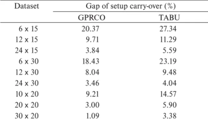
H[SHULPHQWV RI *35&2 DQG 7$%8 7KHVH UHVXOWV VKRZ that the single-plant instances with 15 periods and 6 items obtained a greater effectiveness measure gap with around 20% on average, and this gap falls as well, as the number of items get higher. This fact happens for the gap between *35&2DQG75,DQGIRUWKHRQHEHWZHHQ7$%8DQG75, These values reveal the good performance of the setup car-ry-over with these instances and, in a more general aspect, for the single-plant CLSP. Furthermore, Table 3 shows that for every set of instances, the tabu search proposed LQ>@SHUIRUPHGEHWWHUWKDQ*35&27KHUHIRUHZHFDQ FRQFOXGHE\WKHUHVXOWVWKDW*35&2SHUIRUPHGZHOOIRU single-plant instances, with near results from TABU.

Table 2 7KH DYHUDJH JDSV EHWZHHQ *35&2 DQG 75, VROXWLRQV DQG EHWZHHQ *35&2 DQG *35 VROXWLRQV 7KLV WDEOH SUHVHQWV WKH DYHUDJH JDSVEHWZHHQ*35&2DQG75,$*DQGEHWZHHQ*35&2DQG*35

(AG2) considering the E, W, F, G and X set of instances. Furthermore,

WKLVWDEOHVXPPDULHVWKHDYHUDJHWLPHVRI*35&2$7

Dataset AG1 (%) AG2 (%) AT (sec)

฀ ฀ ฀ ฀

W ฀ ฀ ฀

F ฀ ฀ ฀

G ฀ ฀ ฀

X ฀ ฀ ฀

Table 3&RPSDULVRQWDEOH7KLVWDEOHVVKRZVDYHUDJHJDSVRI*35&2

and the tabu search heuristic proposed in [9]. These gaps are between the carry-over heuristics and the benchmark TRI heuristic. The tabu search average gaps are given in [9]. The dataset is represented by the number of items x number of periods, e.g., 6 x15 represents all instances with 6 items and 15 periods.

Dataset Gap of setup carry-over (%)

*35&2 TABU

6x 15 20.37 27.34

12 x 15 9.71 11.29

24 x 15 3.84 5.59

6x 30 18.43 23.19

12 x 30 8.04 9.48

24 x 30 3.46 4.04

10 x 20 9.21 14.57

20 x 20 3.00 5.90

30x 20 1.09 3.38

4.2. M

-P

CLSP E

At this stage, we tested the heuristic with multi-plant in-stances reported in [14] which consist of 8 sets composed by 120 instances each one resulting in 960 instances. Each set includes 5 instances for every combination of 3, 4, 5, and 6 periods with 3 and 4 plants and with 5, 10 and 15 items. More details about these instances can be found in [14]. The number of initial solutions set for these instances is 1000.

Table 4. Gaps between GPR and linear relaxed solution. The first column of this table presents the set of instances. The second to last columns present, respectively, the average gap between GPR and the linear re-laxed solution and the average time of the heuristic.

Dataset Average Gap (%) Mean Time (sec)

THH 28.04 21.26

THL 28.98 19.97

NHH 24.91 15.62

NHL 25.75 17.33

TLH 8.66 31.76

TLL 8.78 32.38

NLH 8.18 25.76

NLL 8.25 27.95

As expected, the results show that the average gaps for in-stances with high setup time are greater than average gaps for instances with low setup time. This fact also happens for prob-OHPV ZLWK SDUDOOHO PDFKLQHV VHH >@ *35 DQG *35&2 found a feasible solution for every solution for this dataset.

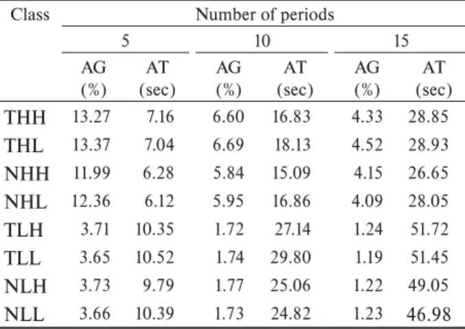
Table 5 shows that in the first four classes of instances whose setup costs are high, the gain in gap comes around 7.8% on average. Moreover, the instances with 5 periods achieved the largest gaps considering all sets of instances. This fact demonstrates that the setup carry-over is more effective with few periods obtaining a significant enhance-ment mainly for the classes with high setup costs. The classes with low setup cost and 5 periods presented a av-erage gap of 3.7%. In all cases, the computational time ZDVVOLJKWO\VXSHULRUZKHQFRPSDULQJ*35&2ZLWK*35 Then the carry-over showed a good performance for the MPCLSP even though for the low setup cost instances the improvement was not substantial.

5. C

In this paper we presented a novel mathematical formu-lation to the MPCLSP with setup carry-over. Furthermore, it addressed an extension of previous research of GRASP with path relinking to solve this problem. The setup carry-over can avoid an extra capacity use through setup saving when the first item to be produced in a given period is the same last produced item in the previous period. Moreover, if a period has extra capacity use, we can transfer the setup of the first item to be produced in this period to the end of the previous period, enabling the saving of this extra ca-pacity. The setup carry-over strategy has been investigated by many researchers and has achieved good results for the single-plant CLSP, even if until now no study for the multi-plant CLSP was developed. Furthermore, the GRASP is potentially useful and one of the most appropriate tech-niques for providing solutions to these models.

To check the robustness of the setup carry-over to the multi-plant CLSP, we have tested different types of CLSP concerning the single and the multi-plant prob-lems. From the results obtained for the MPCLSP with setup carryover, it is observed that the classes with low setup cost have, in general, performed less efficiently than the instances with high setup cost, whose saving was substantial mainly for few period instances. In con-trast, the classes with a single-plant had performed better than the multiplant instances.

Because of the promising results, the approach pre-sented might have potential applications to a variety of lot sizing problems. Further research on the use of setup carry-over should be principally directed toward the CLSP with parallel machines which has similar properties to the MPCLSP.

A

The authors gratefully acknowledge the funding from FAPESP. Furthermore, the authors thank the anonymous referees for valuable suggestions.

R

[1] A. Aggarwal, J. K. Park. Improved algorithms for economic lot size problems. Operations Research. 41: 549-571, 1993.

[2] V. A. Armentano, P. M. França, F. M. B. de Toledo. A network flow model for the capacitated lot-sizing problem.Omega. 27: 275-284, 1999.

[3] D. Briskorn. A note on capacitated lot sizing with setup carry over. IIE Transactions. 38: 1045-1047, 2006.

[4] M. Diaby, H. C. Bahl, M. H. Karwan, S. Zionts. Capacitated lot-sizing and scheduling by lagrangean Table 6 shows that for the high setup cost set of

instances, the average gap is around 28% whereas, for the low setup cost set of instances, the average gap SUHVHQWHG DURXQG 2Q RQH KDQG WHVWV LQ &3/(; with some non relaxed instances with high setup costs showed a very low gap, with around 2%, what shows that WKLVORZHUERXQGLVSRRUIRUWKHVHVHWVRILQVWDQFHV2Q the other hand, most of these instances did not find a solution in reasonable time making dificult the compari-son with the optimal non relaxad instances. Therefore, these results validate the heuristic with setup carry-over for the multi-plant instances demonstrating a very good performance.

Table 5 *DSV EHWZHHQ *35 DQG *35&2 FRQVLGHULQJ WKH QXPEHU RI

periods and different classes of instances. The first column of this table presents the set of instances. The second to last columns present,

respec-WLYHO\WKHIHDVLELOLW\LQGH[WKHDYHUDJHJDSVEHWZHHQ*35DQG*35&2 DQGWKHDYHUDJHWLPHVRI*35&2IRUVHWVZLWKUHVSHFWLYHO\DQG

15 periods.

Class Number of periods

5 10 15

AG (%)

AT (sec)

AG (%)

AT (sec)

AG (%)

AT (sec)

THH 13.27 7.16 6.60 16.83 4.33 28.85

THL 13.37 7.04 6.69 18.13 4.52 28.93

NHH 11.99 6.28 5.84 15.09 4.15 26.65

NHL 12.36 6.12 5.95 16.86 4.09 28.05

TLH 3.71 10.35 1.72 27.14 1.24 51.72

TLL 3.65 10.52 1.74 29.80 1.19 51.45

NLH 3.73 9.79 1.77 25.06 1.22 49.05

NLL 3.66 10.39 1.73 24.82 1.23 46.98

Table 6*DSVEHWZHHQ*35&2DQGRSWLPDOUHOD[HGVROXWLRQFRQVLGHULQJ

the number of periods and different classes of instances. The first col-umn of this table shows the set of instances. The second to last colcol-umns

SUHVHQW UHVSHFWLYHO\ WKH DYHUDJH JDSV EHWZHHQ *35&2 DQG RSWLPDO UHOD[HGVROXWLRQVDQGWKHDYHUDJHWLPHVRI*35&2IRUVHWVZLWKUHVSHF -tively, 5, 10 and 15 periods.

Class Number of periods

5 10 15

AG (%) AG (%) AG (%)

THH 28.19 30.06 31.20

THL 29.87 30.68 31.82

NHH 26.51 28.26 29.10

NHL 26.36 28.91 29.83

TLL 6.96 7.92 8.01

TLL 7.14 8.04 8.10

NLH 6.17 7.46 7.66

[16] P. Porkka, A. P. J. Vepsäläinen, M. Kuula. Multiperiod production planning carrying over set-up time.

International Journal of Production Research. 41(6): 1133-1148, 2003.

[17] M. Sambasivan, C. P. Schimidt. A heuristic procedure for solving multi-plant, multi-item, multi-period capacitated lot-sizing problems. Asia Pacific Journal of Operational Research. 19: 87-105, 2002.

[18] M. Sambasivan, S. Yahya. A Lagrangean-based heuristic for multi-plant, multi-item, multi-period capacitated lot-sizing problems with inter-plant transfers. Computers and Operations Research. 32: 537-555, 2005.

[19] K. X. S. Souza, V. A. Armentano. Multi-item capacitated lot-sizing by a cross decomposition based algorithm. Annals of Operations Research. 50: 557-574, 1994.

[20] C. R. Sox, Y. B. Gao. The capacitated lot sizing problem with setup carry-over. IEE Transactions. 31: 173-181, 1999.

[21] C. Suerie, H. Stadtler. The capacitated lot-sizing problem with linked lot sizes. Management Science. 49: 1039-1054, 2003.

[22] C. S. Sung. A single-product parallel-facilities production-planning model. International Journal of Systems Science. 17: 983-989, 1986.

[23] F. M. B. Toledo, V. A. Armentano. A lagrangean-based heuristic for the capacitated lot-sizing problem in parallel machines. European Journal of Operational Research. 175: 1070-1083, 2006.

[24] W. W. Trigeiro, L. J. Thomas, J. O. McClain. Capacitated lot sizing with setup times. Management Science. 35: 353-366, 1989.

[25] A. Wagelmans, S. Van Hoesel, A. Kolen. Economic lot sizing: an o(nlogn) algorithm that runs in linear time in the wagner-whitin case. Operations Research. 40: 145-156, 1992.

[26] H. M. Wagner, T. M. Whitin. Dynamic version of the economic lot size mode. Management Science. 5: 89-96, 1958.

relaxation. European Journal of Operational Research. 59: 444-458, 1992.

[5] M. Diaby, H. C. Bahl, M. H. Karwan, S. Zionts. A lagrangean relaxation approach for very-large-scale capacitated lot-sizing. Management Science. 59: 1329-1340, 1992.

[6] A. Federgruen, M. Tzur. A simple forward algorithm to solve general dynamic lot sizing models with n periods in o(nlogn) or o(n) time. Management Science. 37: 909-925, 1991.

[7] T. A. Feo, M. G. C. Resende. A probabilistic heuristic for a computationally difficult set covering problem.

Operations Research Letters. 8: 67-71, 1989.

[8] F. Glover. A template for scatter search and path relinking. In Proceedings of AE ‘97: Selected Papers from the Third European Conference on Artificial Evolution, London, UK, pages 3-54, 1998.

[9] M. Gopalakrishnan, K. Ding, J. M. Bourjolly, S. Mohan. A tabu-search heuristic for the capacitated lot-sizing problem with set-up carryover. Management Science. 47: 851-863, 2001.

[10] M. Gopalakrishnan, D. M. Miller, C. P. Schmidt. A framework for modelling setup carryover in the capacitated lot sizing problem. International Journal of Production Research. 33(7): 1973-1988, 1995.

[11] M. Laguna, R. Martí. Grasp and path relinking for 2-layer straight line crossing minimization. Informs Journal on Computing. 11(1): 44-52, 1999.

[12] S. Lozano, J. Larraneta, L. Onieva. Primal-dual approach to the single level capacitated lot-sizing problem.European Journal of Operational Research. 51: 354-366, 1991.

[13] J. Maes, J. O. McClain, L. N. Van Wassenhove. Multilevel capacitated lotsizing complexity and lp-based heuristics. European Journal of Operational Research. 53: 131-148, 1991.

[14] M. C. V. Nascimento, M. C. G. Resende, F. M. B. Toledo. GRASP with path-relinking for the multi-plant capacitated lot sizing problem. European

Journal of Operational Research, accepted for publication, 2008.