Natural Color Scenes Using
Hierarchical Region-Growing and a
Color-Gradient Network
Aldo von Wangenheim
1, Rafael F. Bertoldi
1, Daniel D. Abdala
2,
Michael M. Richter
3, Lutz Priese
4, Frank Schmitt
41Lab for Image Processing and Computer Graphics – LAPIX
Department of Computer Sciences – INE, Universidade Federal de Santa Catarina – UFSC Phone: +55 (48) 3721-9516 (LAPIX), +55 (48) 3721-9117 (Telemedicine)
CEP 88049-200 Florianopolis - SC, Brazil FAX: +55 (48) 3331-9516-R16 {awangenh | fogo}@inf.ufsc.br
2University of Münster, Department of Computer Science Einsteinstrasse 62, D-48149 Münster, Germany Phone: +49 (251) 833-3759, Fax: +49 (251) 833-3755
3Department of Computer Science, University of Calgary Phone: +1 (403) 220-6783, Fax: +1 (403) 284-4707
Calgary, Canada [email protected]
4Institut für Computervisualistik, Universität Koblenz-Landau Phone: +49 (261) 287-2792, Fax: +49 (261)287-100-2792
Postfach 201 602, 56016 Koblenz, Germany {priese | fschmitt}@uni-koblenz.de
Received 29 August 2008; accepted 15 November 2008
Abstract
We present evaluation results with focus on combined image and efficiency performance of the Gradient Network Method to segment color images, especially images showing outdoor scenes. A brief review of the techniques, Gradient Network Method and Color Structure Code, is also presented. Different region-growing segmentation results are compared against ground truth images using segmentation evaluation indices Rand and Bipartite Graph Matching. These results are also confronted with other well established segmentation methods (EDISON and JSEG). Our preliminary results show reasonable performance in comparison to several state-of-art segmentation techniques, while also showing very promising results comparatively in the terms of efficiency, indicating the applicability of our solution to real time problems.
Keywords: color image segmentation, fast segmentation, outdoor scenes, Color Structure Code, Gradient Network Segmentation.
1. I
NTRODUCTIONNatural color scenes, such as outdoor images composed by many colored objects that are acquired under uncontrolled conditions show complex illumination patterns across the same object in the picture. Examples are variations in lightness and specular effects. State-of-the-art region-growing segmenta-tion methods [1,2,3] present two main features that limit their applicability for dealing efficiently with natural scenes:
pa-rameters of such algorithms are stressed in order to try to accomplish a correct segmentation of a large object showing a long continuous gradient of color, typically with a gradual but large color variation, a region leakage of other objects in the image is likely to occur. Then the algorithm is becoming unstable and even inapplicable. x ,QFUHDVHLQFRPSOH[LW\ in order to present more
stable results. This usually demands complex computations to detect segment-correlation clues, such as the usage of additional texture information. This slows down considerably the processing time without being much more stable when extreme color variations are present.
In this paper we present for the first time a ground truth-based objective qualitative validation of our previously pre-sented gradient network approach for image segmentation [4] and analyze its performance in conjunction with anoth-er method [1], providing a novel color scene segmentation approach that is extremely fast. It is intended to be used as a two-step approach that shows satisfactory results when applied to natural color scenes, while not showing poorer performance than state-of-the-art methods. Both empirical validations, the objective qualitative analysis as well as the performance comparison are performed against state-of-the-art segmentation algorithms an presented in detail.
The approach described here is based on a pipeline of two fast segmentation algorithms:
I. A hierarchical region-growing segmentation [1] that generates an over-segmented picture where natural boundaries of objects are preserved.
II. A color gradient based region-growing post-seg-mentation method [4] that starts from an initial pre-segmented image and computes a gradient network that spans the entire image. It finds lo-cally connected gradients that show an organized pattern, representing ordered color variations of a same object. These “organized segment clus-ters” composed of correlated shades of color and light are merged into meta-regions that are then presented as the final segmentation result. One of the most important features of this algorithm is its computational efficiency.
In this paper we present a short review of the Gradient Network Method (GNM), highlighting the characteristics responsible for its performance. The Color Structure Code (CSC) method is also addressed, followed by results ob-tained with this combined approach. A processing time comparison is presented taking into account two different combinations of pre-segmentation region growing algo-rithms with the GNM. It should clarify the main reason
for choosing the CSC as the first stage of this approach. These results are compared against a set of state-of the-art region-growing segmentation algorithms and the results are presented.
Finally we present a discussion that takes into account the applicability of such an algorithm for real-time color image segmentation.
2. O
BJECTIVES ANDV
ALIDATIONM
ETHODOLOGYThe GNM produced promising results from the quali-tative point of view. Since it was developed to provide a stable solution for the segmentation of images contain-ing objects presentcontain-ing changes in shades of color, while maintaining good performance characteristics, we devised a set of experiments with the objective to demonstrate em-pirically that the GNM in conjunction with a fast pre-seg-mentation method is capable of providing an alternative to state-of-the-art segmentation algorithms that is much faster while showing at least the same robustness and seg-mentation quality levels.
We employed the following method:
a) Selected a set of state-of-the-art segmentation algorithms to compare to the performance and segmentation results achieved with GNM. This set is different from the one used in [4].
b) Followed a new empirical ground truth-based validation strategy intended to provide concrete objective qualitative results.
For this purpose, we devised the following procedure:
I. Two well-known segmentation methods to be used as pre-segmentation procedures were cho-sen: CSC [1] and Mumford-Shah [3].
II. Segmentations performed with each of these al-gorithms were compared against ground-truths using Rand [5] and Bipartite Graph Matching (BGM) [6] indexes. For each segmentation method we selected a wide range of segmenta-tion parameters, selected the result considered to be the best one for every pair of image set and segmentation algorithm and generated Rand and BGM scores for the complete set of ground-truths for each image
to any ground truth was allowed. Each of these results was used as an input for the GNM algo-rithm, which also was run with a set of different parameters. The resulting segmentations after post-processing with the GNM were also com-pared against ground-truth images using Rand and BGM indexes.
IV. We compared these results to two other well-es-tablished segmentation methods: JSEG [2] and EDISON [7] also using the ground-truth images and the Rand and BGM indexes.
In this context, the comparison against the EDISON method is new and was chosen because of its quality and robustness. The subjective comparisons against the RHSEG [8] method shown in [4] where not included into this experiment because RHSEG needs user interaction, which can introduce a subjective bias, and is therefore not suited to be tested with the proposed validation methodol-ogy.
For the pre-segmentation step, the parameter used for CSC was threshold = 30 and for Mumford-Shah images were generated with lambda = 600. The parameter ranges and increment steps used for these segmentation methods were the following:
1. CSC: 20 threshold 100, threshold-step = 10;
2. Mumford-Shah: 1000 lambda 15000, lamb-da-step = 500;
3. EDISON: 3 SS 30, SS-step = 1, SR = 8.
4. JSEG is an unsupervised technique and does not require parameters.
The chosen segmentation quality measures for qualita-tive validation [5,6] are described in the Appendix. Each measure was chosen because it is a representative of one of two widely employed segmentation quality metrics: counting of pairs and set matching.
3. G
RADIENTN
ETWORKM
ETHODThe GNM [4] was developed to deal with segmenta-tion problems where objects in the scene are represented by gradually varying color shades, as they often are found in outdoor scenes. This technique employs a novel seg-mentation strategy and was developed for robust and fast image segmentation.
The GNM looks for a higher degree of organization in the structure of the scene through search and identifi-cation of continuous and smooth color gradients. To be able to run over the image and identify these variations of colors, the GNM uses a graph G (V, E) to structure the initial stage of the algorithm. The graph will be used as a structure to guide the algorithm. This strategy is
relat-ed to the approach in [9]. The vertices
V represent regions identified in a previous pre-segmentation. GNM concentrates on regions of high similarity, specifically in the aspect of low color variation. The goal of the pre-seg-mentation with a different algorithm is to obtain groups of pixels with a high degree of similarity represented in a simple way, avoiding possible problems with local noise if the representation would be done individually for each pixel as a vertex.The tests with GNM were performed combining it with a Mumford-Shah functional (MS) based pre-segmentation provided by the Megawave package [10] and with the Color Structure Code (CSC) [1] algorithm. Other tech-niques, such as Watershed [11], could also be employed for the pre-segmentation step. The pre-segmentation al-gorithm must only fulfill the requirement of producing super-segmented results that preserve the main edges. The quality of the pre-segmentation, however, affects the final result as is shown below.
The external pre-segmentation step is followed in GNM by a labeling procedure to convert the segmentation output into a graph G (V, E). The next step is to check all the neigh-borhood relations if they comply to the similarity measure and provide continuous and smooth color gradients. The evaluation of the continuity of the gradients along the paths found in the graph is done by a function fc that takes into account the perception [12] variations. This allows a better evaluation of the similarity in presence of differ-ent luminance in the regions. Regions of continuous and smooth gradients are due to the presence of lighting effects in the scene of an image. With this additional feature, the algorithm becomes more robust when applied to images with such characteristics. Therefore, even when the neigh-borhood contains regions too dark or too illuminated it will search for the best possible gradient path in the graph [4].
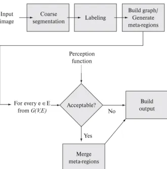
All e E will be evaluated by the chosen similar-ity measure and regions found acceptably similar will be grouped in meta-regions. The resulting meta-regions of the whole process will be the output produced by the GNM segmentation. A high-level structural description of the algorithm can be found in Figure 1.
3.1. B
RIEFA
LGORITHMICD
ESCRIPTION OF THEG
RADI-ENT
N
ETWORKM
ETHODA summarized version of the GNM algorithm is given below:
1. Given a segmented image, a labeling process will be applied and the homogeneous objects in the image will identified.
3. Associate each vertex
VV with an uniquemeta-region m, that will be used to represent and group similar regions and that have a path con-necting them.
4. With the connected graph, select any edge e E
of the graph G(V, E).
4.1. For the current edge, take the two vertices
1, 2 VVV, and verify if they are not al
-ready contained in the same meta-region
m. If so, proceed to 4.4. Else, continue.
4.2. Identify which type of perception, clear or rough, applies to the gradient of color be-tween verticesv v V
2 1, .
4.3. According to the identified perception, evaluate through a similarity measure if the gradient between these vertices is smaller than the threshold defined for the cur-rr rent perception. If it is, the meta-regions
m1 andm2 containing each of the vertices are merged into a new meta-region mn. Otherwise, do nothing.
4.4. Mark this edge as verified. Select an edge that has not been yet verified and go back to the first step of this group of instruc-tions. If there is none, follow to step 5.
5. With the meta-regions found in the former steps build the output image, as each meta-region now represents what is considered an object in the scene of the image by the algorithm. Represent
each pixel in the a meta-region by the mean value of the pixels of the meta-region.
For a more formal description of this algorithm we re-fer to [4].
4. T
HEC
OLORS
TRUCTUREC
ODEThe Color Structure Code (CSC) [1] was developed at the CS Department of the University of Koblenz, Germany. CSC was aimed at the segmentation of scenes from a camera in a car in motion for real-time road sign recognition. The CSC is a region growing algorithm that uses a hierarchical topology formed by islands, a topol-ogy type introduced by [13]. These islands have different levels, as shown in Figure 2. A level 0 island is a hexa-gon, composed by the 6 vertex points around a central point. During the process, some islands overlap others such that leveln+1 islands are composed by seven level
n overlapped islands. This will be repeated until an island spans the entire image.
Build graph/ Generate meta-regions Input
image Labeling
Build output
Merge meta-regions Coarse
segmentation
For every e E from G(V,E)
Perception function
Acceptable?
Yes No
Figure 1. Diagram displaying the GNM process.
Island of level 1
Island of level 2
Island of level 0
pixel
Figure 2. CSC’s hierarchical island structure. [1]
As a first step, the whole image will be partitioned into level 0 islands. A merging step, where the islands will grow and overlap iteratively, will follow. After the grouping step, a split step is performed, where some corrections will take place through the use of global information. In this way, CSC combines a local information step in the merging process and a global information evaluation in the split step, looking for segmenting regions with the highest simi-larity.
conse-quence, found in most algorithms, sensitive regions might be swallowed or more cautious parameters might produce many more segments than would be useful. We will show that the CSC shows good performance and reliability re-garding outdoor images when employed as a pre-process-ing step for the GNM, which then performs the sensitive global gradient-based region grouping actions.
5. A
CHIEVINGE
FFICIENCY ANDR
OBUSTNESS High speed performance segmentation algorithms have been investigated to satisfy the demands from appli-cations that require real-time results. Fast segmentation processes could be used in several situations, like motion detection in video frames or autonomous vehicle guidance [1]. Another application would be to guide surgery and other medical procedures. An example is given in [14], where segmenting a carotid artery is a useful step in medi-cal imaging. Efficiency requirements can also be found in several other areas. [15] presents a technique developed for real time applications as space-weather analysis. In [16] an approach is proposed to track players in a soccer pitch. Fast segmentation approaches are a recurrent topic and several optimizations or specializations over known techniques have been developed [17,18,19].While several algorithms can achieve good results ne-glecting speed, GNM and CSC are both generic segmenta-tion techniques that provide a reasonably good perform-ance.
5.1. G
NMC
OMPLEXITYI
SSUESGNM achieves performance through a set of inte-grated strategies. First, an optimized labeling algorithm performs the initial processing of the pre-processed image and ensures a fast solution to this intermediate step. The complexity of the used labeling algorithm is O(n²).
After classifying the information in the labeling, the construction of the graph takes place. This will structure the information since every region found by the labeling
will correspond to a vertex of the graph. The graph gen-eration step has a complexity of O(n). To improve the per-formance and avoiding redundant loops, the mean color value computation for every region and the conversion to the HSI color space are done together with the graph gen-eration step.
To merge regions presenting similar perception [12], the graph is then traversed Since this step depends solely on the number of edges, its complexity is O(m).
GNM total complexity is O(n² + n + m), where n is the number of vertices and m the number of edges. This method presents a simple solution that is only dependent of the image size and the scene complexity of the result-ing pre-processed image. It is important to note, though it can’t be accounted in the GNM complexity, that the chosen algorithm for the pre-segmentation has an effect on the total time of processing in this approach. A proper technique must be selected here.
5.2. P
RE-S
EGMENTATIONI
SSUESAs our main focus here is to obtain robust results com-bined with high performance, we have chosen the Color Structure Code (CSC) [1] as our pre-segmentation tech-nique.
Though CSC is focused on speed and was developed for specific purposes, it still achieves good results in terms of general robustness and proves to be a good solution in generic cases too. The islands of similarity approach fits nicely with the expected feature for GNM starting point, i.e. the regions of very similar characteristics avoiding leak-ages.
As a main source for quality and performance compar-ison, we used the traditional Mumford-Shah Functional implementation supplied by the Megawave [10] image processing package. The behavior of this method is well known and documented and was considered for a long time the best choice for quality comparisons.
6. R
ESULTS ANDD
ISCUSSIONTo empirically validate the approach, 17 outdoor im-ages showing different color and texture characteristics where processed with all methods. To allow performance comparisons, all tests were run on the same computer.
The adoption of the Berkeley’s image dataset [20] was a necessary and desirable choice since it is a well known dataset with the added features of ground truth (hand seg-mented) images for every set that will help us in future quality evaluations.
The combined segmentation techniques used in the following tests were: GNM applied over pre-segmented images by CSC, with a threshold equal to 30 and GNM applied over pre-segmented images by a Mumford-Shah
functional based segmentation, with lambda equal to 600. The GNM parameters were iterated over a range of rea-sonable values and the results showing the best Rand and BGM indexes were chosen.
For all other four results, CSC and MS alone, and JSEG and EDISON, the parameters were not preset, but were iterated over a range of reasonable values and the results showing respectively the best Rand and BGM in-dexes were chosen. It was allowed for the best results ac-cording to Rand and BGM to be different.
6.1. P
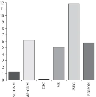
ERFORMANCEThe mean execution time for all images with each method is shown in Figure 4. The total execution time for each set with every selected algorithm is shown in Table 1. This time was obtained by the difference of two time stamps, one in the start and one in the end of the execution process of each algorithm. Mean and standard deviation for every set are also displayed.
0 2 4 3
1 6 5 8 10 9
7 12 11
CSC
+
G
N
M
MS+GN
M
CSC MS JSEG
EDISON
Figure 4. Chart comparing mean execution times in seconds.
The computer the tests were run on is an AMD Athlon 64, 2.2 GHz with 512MB RAM memory and the time unit is seconds. Figure 5 shows image results obtained with GNM combined with both CSC and Mumford-Shah. As the Table 1 shows, the combination of CSC and GNM shows results with a mean value of about 1.2 seconds, which is only slower than CSC. This was expected, consid-ering the cumulative times of CSC+GNM.
The mean time for CSC+GNM is several times shorter than Mumford-Shah (including MS+GNM), EDISON and JSEG, which is the slowest of all. There is little standard deviation among the times obtained for CSC+GNM, while
again in accordance with the exception of CSC alone, all other techniques show higher standard deviations.
Comparing CSC+GNM with MS+GNM, we see that GNM takes longer in the CSC+GNM case than in the MS+GNM case. This occurs because of the existence of several small image fragments that are produced by CSC which are not found in Mumford-Shah segmentations, re-sulting in much more graph vertices to be evaluated.
It is important to notice, however, that GNM has a very stable performance in both cases, with little deviation among the tests cases.
6.2. Q
UALITYFigure 5 shows segmentations of complex illuminated objects, as the sky in the 368078 set or the red roof of the church in the 118035 set. Higher resolution images, com-parisons among several algorithms and more results can be found in http://www.lapix.ufsc.br/fast .
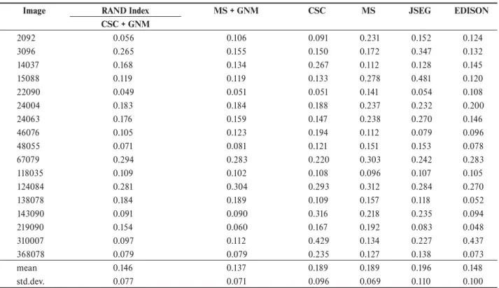
Tables 2 and 3 show the results of the objective qualita-tive validation of the segmentations using the RAND and BGM indexes. We have included the mean results for each image and method for comparison and the standard devia-tion as a measure of robustness.
For the RAND index both combinations of the GNM with pre-segmentations showed the best mean results and also the highest robustness, presenting the lowest standard deviation among the results.
CSC+GNM is the second best, being behind only MS+GNM and slightly better than EDISON.
For the BGM index, the combinations of the GNM with pre-segmentations scored at place 3 and 4. The best results were achieved by the EDISON method, being fol-lowed closely by the CSC alone.
Original Ground-truth CSC+GNM M&S+GNM
Table 1. The total execution times for 17 Berkeley dataset images processed using the techniques is listed in Results and Discussion. In the GNM cases, the time consumed by GNM is shown in parenthesis. Landscape images dimensions are 481 x 321 pixels and portrait images are 321x481 pixels. The mean time, standard deviation in seconds and standard deviation in percent for every algorithm test are displayed in the last lines of the table.
Image Execution Times in Seconds MS + GNM CSC MS JSEG EDISON
CSC + GNM
2092 0.625 (0.547) 5.422 (0.500) 0.078 4.782 9.30 4.52
3096 0.719 (0.641) 5.313 (0.547) 0.063 4.641 7.49 2.15
14037 0.625 (0.547) 9.203 (0.516) 0.062 8.172 11.14 4.81
15088 0.656 (0.547) 5.547 (0.515) 0.078 5.063 26.50 7.14
22090 0.609 (0.515) 5.187 (0.531) 0.078 4.687 9.06 5.12
24004 0.719 (0.625) 5.609 (0.609) 0.094 4.969 10.78 6.00
24063 0.594 (0.516) 5.203 (0.453) 0.062 4.828 9.08 3.07
46076 0.641 (0.547) 5.329 (0.516) 0.078 4.766 11.09 5.89
48055 0.828 (0.719) 5.563 (0.641) 0.094 4.828 14.22 7.18
67079 0.672 (0.578) 5.360 (0.516) 0.079 4.937 12.33 6.77
118035 0.702 (0.593) 6.093 (0.531) 0.078 5.375 9.39 3.78
124084 0.657 (0.563) 5.109 (0.562) 0.078 5.375 9.39 11.39
138078 0.750 (0.656) 6.030 (0.562) 0.078 5.360 14.36 5.53
143090 0.641 (0.547) 5.047 (0.578) 0.078 4.469 12.91 4.41
219090 0.719 (0.625) 5.359 (0.593) 0.093 4.735 11.84 5.23
310007 0.641 (0.531) 5.609 (0.500) 0.094 5.031 9.89 7.28
368078 0.734 (0.672) 5.093 (0.593) 0.078 4.547 12.58 7.20
mean 0.678 (0.586) 5.652 (0.545) 0.079 5.092 11.844 5.734
std.dev. 0.061 (0.06) 0.962 (0.047) 0.010 0.840 4.240 2.096
% std.dev. 9% (10%) 17% (9%) 13% 16% 36% 37%
Table 2. Segmentation quality results for 17 different Berkeley Dataset outdoor images according to the Rand Index
Image RAND Index MS + GNM CSC MS JSEG EDISON
CSC + GNM
2092 0.056 0.106 0.091 0.231 0.152 0.124
3096 0.265 0.155 0.150 0.172 0.347 0.132
14037 0.168 0.134 0.267 0.112 0.128 0.145
15088 0.119 0.119 0.133 0.278 0.481 0.120
22090 0.049 0.051 0.051 0.141 0.054 0.108
24004 0.183 0.184 0.188 0.237 0.232 0.200
24063 0.176 0.159 0.147 0.238 0.270 0.146
46076 0.105 0.123 0.194 0.112 0.079 0.096
48055 0.071 0.081 0.121 0.151 0.153 0.078
67079 0.294 0.283 0.220 0.303 0.242 0.283
118035 0.109 0.102 0.108 0.096 0.107 0.105
124084 0.281 0.304 0.293 0.312 0.284 0.270
138078 0.184 0.189 0.109 0.157 0.118 0.052
143090 0.091 0.090 0.316 0.218 0.235 0.094
219090 0.154 0.060 0.167 0.192 0.083 0.048
310007 0.097 0.112 0.429 0.134 0.227 0.437
368078 0.079 0.079 0.235 0.127 0.138 0.073
mean 0.146 0.137 0.189 0.189 0.196 0.148
7. C
ONCLUSIONS ANDD
ISCUSSIONWe have empirically shown that the quality of the seg-mentations generated by our two-step approach is very promising and comparable to segmentations generated by state-of-the-art methods that were available for compari-son when this paper was being written. On the other side, the segmentation time of a given image when processed by our suggested two-step method was shown to be consider-ably less than when other approaches were used or when the Gradient Network Method step was used in combina-tion with more tradicombina-tional segmentacombina-tion approaches such as the Mumford-Shah functional.
Considering that CSC + GNM is five times faster than EDISON, which is the method that has shown the best quality scores as a standalone approach, it is noticeable that the CSC + GNM segmentation quality scores are so high, being even better than the EDISON according to the Rand index. CSC + GNM also presented a stable behavior, both in performance, showing little variation in processing time, and also in quality, showing little varia-tion in the Rand index, thus providing extremely robust image segmentation results.
The EDISON implementation provided the best BGM index scores, while JSEG provided the worst ones. Both combined GNM approaches remained in the middle. This is a good enough score, when considering that the
GNM is being compared to state-of-the-art segmentation methods. On the other hand, as the results provided in http://www.lapix.ufsc.br/fast show, the BGM method tends to prefer bigger regions, even if a region overlaps partially into another. This leads to results showing under-segmen-tations with segment leakage receiving a higher score than with the Rand method. We have developed our method explicitly to analyze rigorously region borders in order to avoid such leakages, even if some over-segmentation is left behind. This can be one reason for the poorer performance according to the BGM index. This would also explain why the CSC alone scored second best and even showed the best robustness according to this same validation index.
The Gradient Network Method is a segmentation post-processing method that is independent of the region-grow-ing method that is applied to generate the super-segment-ed input image. This has been shown by the comparison between the results produced using the CSC method and when the Mumford-Shah functional is used as the pre-processing step. It is interesting to note that the quality of the final results is very similar, although the intermedi-ate segmentation results of the Mumford-Shah functional are sometimes of a “prettier” quality. The processing time, however, is extremely shorter when a rapid approach like the CSC, which was originally developed for real-time color segmentation, is used. This shows that the
process-Table 3. Segmentation quality results for 17 different Berkeley Dataset outdoor images according to the BGM Index.
Image BGM Index
CSC + GNM MS + GNM CSC MS JSEG EDISON
2092 0.124 0.129 0.114 0.262 0.056 0.103
3096 0.138 0.033 0.010 0.045 0.220 0.048
14037 0.175 0.340 0.017 0.187 0.275 0.026
15088 0.073 0.109 0.084 0.170 0.375 0.114
22090 0.243 0.284 0.242 0.147 0.214 0.204
24004 0.430 0.463 0.412 0.557 0.555 0.424
24063 0.104 0.089 0.037 0.306 0.326 0.054
46076 0.318 0.409 0.245 0.331 0.259 0.072
48055 0.114 0.139 0.198 0.336 0.402 0.081
67079 0.104 0.124 0.217 0.145 0.213 0.117
118035 0.202 0.275 0.192 0.205 0.238 0.066
124084 0.610 0.702 0.279 0.329 0.624 0.388
138078 0.394 0.419 0.147 0.298 0.244 0.053
143090 0.206 0.206 0.173 0.465 0.512 0.157
219090 0.338 0.211 0.205 0.314 0.214 0.195
310007 0.137 0.181 0.086 0.292 0.340 0.038
368078 0.355 0.385 0.154 0.489 0.455 0.314
mean 0.239 0.264 0.165 0.287 0.325 0.144
ing step with the Gradient Network Method allows us to rely on very fast pre-segmentation methods that reduce the total processing time while producing end-segmentations of good quality, even if the pre-processing method is not so good as more traditional approaches.
From the performance point of view, we did not ana-lyze the methods under varying parameter settings, even if we processed each image under approximately 30 differ-ent parameter settings for each method except JSEG. Our focus was quality with speed, thus we considered only the segmentation result which presented the best quality un-der each of the metrics to compute the performance. So, the processing time shown in our result tables is always the time it took to process the segmentation that showed the best quality score.
Further improvements, however, could still be achieved in terms of efficiency with the use of a graphics process-ing unit for performprocess-ing the necessary computations of the involved algorithms. This kind of technology, referred as General-Purpose Computing on Graphics Processing Units (GPGPU), would achieve better results, probably real-time ones. This could make the combination of CSC and GNM a feasible solution to real-time applications that deal with outdoor scenes, as robotics or traffic monitoring applications. Preliminary results not reported and shown here gave some promising perspectives.
When the experiments described in this paper were be-ing performed, a new variant of the Mumford-Shah algo-rithm was published, that is described as overcoming one of the most important shortcomings of Mumford-Shah, namely the long processing time [21]. We did not have the opportunity to implement and test this new variation, but since CSC is in average 64 times faster than the tradition-al Mumford-Shah, showing a mean segmentation time of 0.079s compared to the mean segmentation time of 5.092s presented by the standard Mumford-Shah implementation, while presenting the same mean Rand index of 0.189 and a better BGM index of 0.165 against the BGM index of 0.287 of Mumford-Shah, we think it is still a better choice for the pre-segmentation step, even if faster versions of the Mumford-Shah algorithm are appearing.
A
CKNOWLEDGEMENTSDaniel D. Abdala thanks CNPq-Brazil for a Ph.D scholarship, and Professor Xiaoyi Jiang for his support during the first months of the Ph.D. work at the University of Münster.
The authors also wish to thank Antônio Sobieransky from the Lab for Image Processing and Graphic Computing – LAPIX for editing and updating the site which presents additional material from this work.
R
EFERENCES[1] V. Rehrmann, L. Priese. Fast and Robust Segmentation
of Natural Color Scenes. ACCV. (1): 598-606, 1998.
[2] Y. Deng, B. S. Manjunath. Unsupervised segmentation of color-texture regions in images and video. IEEE Transactions on Pattern Analysis and Machine Intelligence. 23(8): 800-810, 2001.
[3] D. Mumford, J. Shah. Optimal approximations by piecewise smooth functions and associated variational problems, Commun. Pure Appl. Math. 42: 577-684, 1989.
[4] A. V. Wangenheim, R. Bertoldi, D. Abdala, M. M. Richter. Color image segmentation guided by a color gradient network. Pattern Recognition Letters. 28: 1795-1803, 2007.
[5] W. M. Rand. Objective criteria for the evaluation of clustering methods. Journal of American Statistical Association. 66: 846-850, 1971.
[6] X. Jiang, C. Marti, C. Irniger, H. Bunke. Distance measures for image segmentation evaluation. EURASIP Journal on Applied Signal Processing. 1-10, 2006.
[7] D. Comaniciu, P. Meer. Mean shift: A robust approach toward feature space analysis. IEEE Transactions on Pattern Analysis and Machine Intelligence. 24(5): 603-619, 2002.
[8] J. C. Tilton. D-dimensional formulation and implementation of recursive hierarchical segmentation. Disclosure of Invention and New Technology: NASA Case Nº GSC 15199-1, May 2006.
[9] A. Trémeau, P. Colantoni. Regions adjacency graph applied to color image segmentation. IEEE Trans. on Image Processing. 9(4): 735-744, 2000.
[10] Megawave image processing package. http://www. cmla.ens-cachan.fr/Cmla/Megawave/, Sept 2006.
[11] L. Vincent, P. Soille. Watersheds in digital spaces: An efficient algorithm based on immersion simulations. IEEE Transactions on Pattern Analysis and Machine Intelligence. 13: 583-598, 1991.
[13] G. Hartmann. Recognition of hierarchically encoded images by technical and biological systems. Biological Cybernetics. 57(1–2): 73-84, 1987.
[14] D. Y. Kim, J. W. Park. Connectivity-based local adaptive thresholding for carotid. Image and Vision Computing. 23(14): 1277-1287, 2005.
[15] T. D. de Wit. Fast Segmentation of Solar Extreme Ultraviolet Images. Solar Physics. 239(1-2): 519-530, 2006.
[16] P. Figueroa, N. J. Leite, R. Barros. Background recovering in outdoor image sequences: an example of soccer players segmentation. Image and Vision Computing. 24(4): 363-374, 2006.
[17] Y. Pan, J. D. Birdwell, Djouadi S. Efficient Implementation of the Chan-Vese Models Without Solving PDEs. Multimedia Signal Processing 2006 IEEE 8th Workshop. Pages 350-354, ANO.
[18] K. Y. Wong, M. E. Spetsakis. Tracking based motion segmentation under relaxed statistical assumptions. Computer Vision and Image Understanding. 101(1): 45-64, 2006.
[19] H. Sun, J. Yang, M. Ren. A fast watershed algorithm based on chain code and its application in image segmentation. Pattern Recognition Letters. 26(9): 1266-1274, 2005.
[20] D. Martin, C. Fowlkes, D. Tal, J. Malik. A database of human segmented natural images and its application to evaluating segmentation algorithms and measuring ecological statistics. In Proceedings of the 8th International Conference on Computer Vision. pages 416-423, 2001.
[21] C. V. Alvino, A. J. Yezzi. Fast Mumford-Shah segmentation using image scale space bases. Proc. SPIE, 6498, 64980F, 2007, DOI:10.1117/12.715201.
Appendix
A S
EGMENTATIONQ
UALITYM
EASURESTo allow the objective segmentation quality validation, we selected two well-known different objective ground-truth-based segmentation quality measures and developed a validation strategy to compare our results against stand-ard segmentation approaches.
There are several approaches to calculate these dis-tance measures. Two widely used kinds of disdis-tances are estimated respectively by counting of pairs and by set matching. In our tests, we used one measure of each these kinds: Rand [5] and Bipartite graph matching (BGM) [6], respectively a pair-counting and a set-matching measure.
A brief description of both quality measures is given below.
A.1 R
ANDI
NDEXThe Rand index [5] is a similarity measure specially developed to evaluate the quality of clustering algorithms by comparison with other clustering results or with a golden standard (in our case, ground-truths). To compare
two clustering results C1={c11, c12, ..., c1N} and C2= {c21,
c22,..., c2M} over the same image P = {p1, p2, ..., pK} where each element of C1 or C2 is a subset of P and c1j = {p1j,
p2j, ..., pLj}, the following quantities are calculated: N
1. 11- the number of pixels in the same cluster in both C1 and C2.
N
2. 00 - the number of pixels in different clusters both in C1 and C2.
The rand index is so defined by eq. A.I
11 00
( 1, 2) 1
( 1)
2
N N
R C C
n n
A.I
To compute the quantities N11 and N00 one must iter-ate over the entire image for each pixel in order to evaluiter-ate the conditions defined above given an O(n4) algorithm. A
clever approach is to use the method where a matching matrix is used to summarize the occurrences of pixels in the respective classes. The matching matrix is constructed allocating each cluster from the clustering C1 to a row and each cluster from clustering C2 to a column. The matrix cells are then defined as the intersection of the clusters specifying each row and column. If the matching matrix
has kxl size each cell can be defined as mij =|ci cj|, ci C1, cj C2.
The quantities N11 and N00 can be computed in terms of the matching matrix as follows:
2 11
1 1
1
2
k l ij i j
N m n A.II
2 2 2 2 00
1 1 1 1
1
2
k l k l
i j ij
i j i j
where n is the cardinality of P and ni and nj are the
cardi-nality of the clusters c1i and c2j.
A.2
BIPARTITE GRAPH MATCHING
TheBGM index [6] computes an one-to-one correla-tion between clusters at the same time trying to maximize their relationship. It considers each cluster of the C1 and C2 clustering as vertices of a bipartite graph. Edges are added between each vertex of the two partitions and they
are valued as |c1i c2j|, a value that can be directly ex-tract from the matching matrix. Then the maximum-weight bipartite graph is defined as the subgraph {(c1i1,c2j1), ...,
(c1ir,c2jr)} where only the edges from c1ito c2j with maxi-mum weight are present. After all max-valued edges were found the overall graph weight is calculated by sum of all remaining edge weights.
( 1, 2) 1 w
BGM C C
Original Ground-truth CSC+GNM M&S+GNM
Figure 5. Examples of the image results obtained by GNM, combined with both CSC and Mumford-Shah. The first row corresponds to image number 368078 and the second row corresponds to 118035 from Berkeley image dataset.
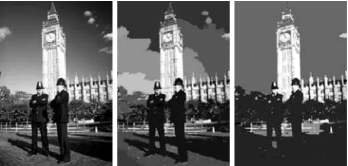
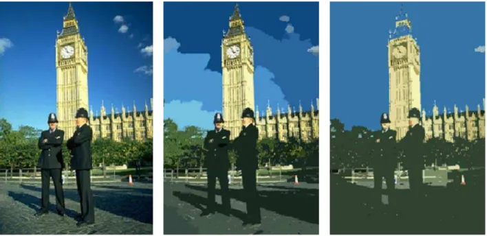
Figure 3. CSC results when processing a complex outdoor image. From left to right: the original image, a cautious approach and an aggressive approach.