Evelise R. Corbalan Góis
[email protected] University of São Paulo School of Engineering, São Carlos 13566-590 São Carlos, SP, BrazilLeandro F. de Souza
[email protected] University of São Paulo Mathematics and Computing Sciences Institute 13560-970 São Carlos, SP, BrazilAn Eulerian Immersed Boundary
Method for Flow Simulations over
Stationary and Moving Rigid Bodies
The fluid flow over bodies with complex geometry has been the subject of research of many scientists and widely explored experimentally and numerically. The present study proposes an Eulerian Immersed Boundary Method for flows simulations over stationary or moving rigid bodies. The proposed method allows the use of Cartesians Meshes. Here, two-dimensional simulations of fluid flow over stationary and oscillating circular cylinders were used for verification and validation. Four different cases were explored: the flow over a stationary cylinder, the flow over a cylinder oscillating in the flow direction, the flow over a cylinder oscillating in the normal flow direction, and a cylinder with angular oscillation. The time integration was carried out by a classical 4th order Runge-Kutta scheme, with a time step of the same order of distance between two consecutive points in x direction. High-order compact finite difference schemes were used to calculate spatial derivatives. The drag and lift coefficients, the lock-in phenomenon and vorticity contour plots were used for the verification and validation of the proposed method. The extension of the current method allowing the study of a body with different geometry and three-dimensional simulations is straightforward. The results obtained show a good agreement with both numerical and experimental results, encouraging the use of the proposed method.
Keywords: Immersed Boundary Method, lock-in phenomenon, high order finite difference schemes
Introduction
1The Computational Fluid Dynamics (CFD) research area increases every day. The main reason is the development in the processing and storage capacities of the computers. However, the main studies in this area are restricted to simple geometries. The numerical studies of flow over bodies with complex geometries, stationary or not, require a mesh and numerical code that is able to reproduce the physics of the flow. Normally the type of meshes adopted coincides with the boundaries of the body. An alternative method is the use of approximations where the boundaries of the body do not need to coincide with the computational mesh, allowing the use of a Cartesian grid. The great challenge of these methods is the use of approximations that assure both accuracy and numerical efficiency.
One of the most cited techniques that have adopted the idea of Cartesian grid for the simulation of flows over bodies with complex geometries is the Immersed Boundary Method (IBM). This method was introduced by Peskin in 1972. His research concerns an incompressible flow in a region with immersed bodies which moved according to the flow and the forces acting on them. The great advantage in his method is that the Navier-Stokes equations are solved in Cartesian grids. In his study the elastic bodies are modeled by a force added to the Navier-Stokes equations as a source term and this force is calculated according to the body configuration. To link the body with the flow, since the mesh points do not need to coincide with the body points, a function analogous to delta function is introduced. The mathematical fundamentals of the IBM can be found in Peskin (2002).
Goldstein et al. (1993) developed a different way to calculate the force field generated by the immersed body, suggesting an iterative control with two constants. In their approximation one can verify that the method works as a harmonic damped oscillator, with one constant for the spring and another for the viscous damper. The main difference between their method and the method proposed by Peskin (1972, 1977) is that the former was developed to solve problems with rigid bodies, while the latter can work with elastic bodies as well.
Paper accepted August, 2010. Technical Editor: Francisco Ricardo Cunha
Saiki and Biringen (1996) used the method proposed by Goldstein et al. (1993) combined with a 4th order code. Their test case was a flow over either a stationary or a moving cylinder. According to the authors, the use of the finite difference method suppressed the numerical oscillations caused by the forcing term found by Goldstein et al. (1993), who used a spectral method. Their numerical simulations were carried out for Reynolds numbers ranging from 25 to 400. Their numerical results suggest that when the Reynolds number is high, the forcing term should be imposed at all internal points of the body, instead of only at the boundaries. Their results were compared with other experimental numerical results, showing a good agreement.
Mohd-Yusof (1997) proposes an Immersed Boundary Method that allows the study of flows over complex geometry bodies using pseudo-spectral methods. An advantage is that it is possible to join a high order of accuracy, due the pseudo-spectral apply, with the study of flows over complex geometry bodies. Another advantage is that the proposed scheme does not need any ad-hoc constant to be set.
Linnick (1999) used the Immersed Boundary Method for transitional flows simulations. His objective was to investigate active flow control using actuators. The actuators were modeled using Immersed Boundary Methods. The vorticity-velocity formulation was used and the method was verified by simulations of flow over a square and a circular cylinder, flow over a cavity and a boundary layer flow with a distributed roughness at the wall. Lai and Peskin (2000) present an Immersed Boundary Method with 2nd order of accuracy. The method was tested with a flow over a cylinder of circular section. The influence of numerical viscosity on the results was analyzed by comparing the results with the first-order code Peskin (1972, 1977). A question that may arise when using their method with different Reynolds numbers concerns how the scheme performs. In other words, it is important to verify whether the numerical method interferes in the physics, especially for high Reynolds number flows. Their results show that with the 2nd order method, the physics is more accurately resolved and it is possible to obtain more stable solutions.
Linnick and Fasel (2003) used a special treatment of the derivatives in the fluid/body interface in their Immersed Boundary Method. The spatial derivatives were calculated using 4th order compact finite difference schemes. Their results assured that the 4th order truncation error was maintained in their studied cases.
Lima e Silva et al. (2003) developed an Immersed Boundary Method and presented results of a flow over a circular cylinder. In their method the force field calculation is performed using the Navier-Stokes equations applied to Lagrangian points and then distributed over an Eulerian grid. The advantage of their method is that the force field calculation is carried out without the need of ad-hoc constants.
An interesting phenomenon may occur analyzing flows around bodies. When a flow over a blunt body becomes unsteady, a vortex shedding can be observed. If the body oscillates at given frequency and amplitude, the flow can be influenced by this oscillation. As a consequence of the induced vortex shedding resonance, the body oscillations can reach sufficient amplitudes such that both body and wake reach the same frequency oscillation values. This is called lock-in phenomenon, discovered over three hundred years ago by Christian Huygens (Burrowes, 2005). The vortex lock-in phenomenon is also referred to as vortex lock-on, phase locking, mode locking, and wake capture. The presence of certain sound fields was also found to cause vortex lock-in. This phenomenon will be used for verification and validation of the present method. Therefore, a short review of this phenomenon is given below. Griffin and Ramberg (1976) studied experimentally the wake of a cylinder vibrating in line with an incident steady flow. All the experiments reported were performed at Reynolds number Re = 190. In their study some bounds for the lock-in regime within wind-tunnel measurements were obtained. The shedding frequency of the stationary cylinder was measured and the cylinder was then oscillated at various frequencies and amplitudes. At each frequency, the amplitude of oscillation was increased until the vortex-shedding frequency had become synchronized with the cylinder motion. The lock-in range for the in-line vibrations extended from about 120% to nearly 250% of the Strouhal frequency.
Choi et al. (2002) investigated the effects of a flow over a cylinder with angular oscillation. The simulations were performed at Reynolds number Re = 100. It was shown that the forcing-frequency range of lock-in became wider as the rotational speed increased. Their study also shows that the lowest values of the mean drag and the amplitude of the lift fluctuations occurred close to the lock-in region. It was also observed that the amount of drag reductions was strongly dependent on the Reynolds number.
The main objective of this work is to present a new technique to calculate the forcing terms added at the governing equations in the Immersed Boundary Method. Numerical Simulations of fluid flow over circular cylinder were used as test cases, and the lock-in phenomenon was also verified. This paper is divided as follows: Formulation and Numerical Method are presented at the next section, followed by Results and Discussion, where the simulations results are discussed and compared with other experimental and numerical results from. Finally the Conclusions are presented.
Nomenclature
Re = Reynolds Number of the air flow, dimensionless u = velocity component in the streamwise direction x
v = velocity component in the normal direction y t = time
p = pressure
x = spatial coordinate in streamwise direction y = spatial coordinate in normal direction F x = forcing term in the streamwise direction x
Fy = forcing term in the normal direction y Cd = drag coefficient
Cl = lift coefficient F = oscillation frequence A = oscillation amplitude rt = relaxation term
f = ramp function
Greek Symbols
ω = vorticity δ = variable value
α = maximum rotation angle
Subscripts
l lift
d drag
x streamwise direction
y normal direction
0 begin of domain
max end of domain
Formulation and Numerical Method
In the present study, the governing equations are the incompressible unsteady Navier-Stokes equations with constant density and viscosity. They consist of the momentum equations given by:
(1)
(2)
and the continuity equation given by:
(3)
where u and v are the velocity components in the streamwise x and
in the normal direction y, respectively, p is the pressure, Fx and Fy
are the forcing terms used by the Immersed Boundary Technique and the Laplacian term is given by:
(4)
where Re is the Reynolds Number defined by:
(5)
where U∞is the reference velocity, D is the cylinder length diameter and ν is the kinematic viscosity.
The vorticity is here defined as the negative curl of velocity vector. Taking the curl of the momentum equations, the vorticity transport equation can be obtained by:
(6)
Taking the definition of vorticity and the continuity equation, it is possible to obtain the Poisson equation for v velocity component:
2
(
)
(
)
,
x
u
uu
vu
p
u
F
t
x
y
x
∂
∂
∂
∂
+
+
= −
+ ∇ +
∂
∂
∂
∂
Re
,
ν
U D
∞=
2
(
)
(
)
.
x
z z z
z
y
F
F
u
v
t
x
y
y
x
ω
ω
ω
ω
∂
∂
∂
= −
∂
−
∂
+ ∇
+
−
∂
∂
∂
∂
∂
2(
)
(
)
,
yv
uv
vv
p
v
F
t
x
y
y
∂
+
∂
+
∂
= −
∂
+ ∇ +
∂
∂
∂
∂
0
u
v
x
y
,
∂
+
∂
=
∂
∂
2 2 2 2 21
,
Re
x
y
⎛
∂
∂
⎞
∇
=
⎜
+
⎟
∂
∂
(7)
All variables are dimensionless quantities. They are related to the dimensional variables by:
(8)
The dimensionless frequency adopted in the cylinder oscillation cases is:
(9)
where fe is the cylinder oscillation frequency and fo is the natural
vortex shedding frequency.
Figure 1 shows the computational domain. The boundary conditions are: at the inflow boundary (x = x0), the velocity and
vorticity components are specified; at the outflow boundary (x = xmax), the second derivative of the velocity and vorticity components
in the streamwise direction is set to zero and, at the upper and lower boundaries, the derivative of v in the y direction is set to zero. The number of points adopted in all simulations was 641 and 497 in the x and y directions, respectively. The distance between two consecutive points was dx = dy = 0.03, and the time step was dt = 0.006. The cylinder has a radius of R = 0.5 and the cylinder center position (initial center position in the cases of cylinder with oscillating) is shown in Fig. 1.
Figure 1. Computational domain.
Three damping zones are used in the simulations to force the disturbances to gradually decay to zero. The basic idea is to multiply the vorticity components by a ramp function f after each step of the integration scheme. This technique has been proved by Kloker et al. (1993) to be very efficient in avoiding reflections that could arise
from the boundaries when simulating unsteady flows. Using this technique, the vorticity component between x1and x2 is:
2 2
2 2
.
z
u
v
x
y
x
ω
∂
∂
+
∂
= −
∂
∂
∂
(10) z( , , )
x
*z( , , ),
where ωz*(x,y,t) is the disturbance vorticity component that arises from the time integration scheme and f is a ramp function that ranges smoothly from 1 to 0. The implemented function, in the x direction is:
(11)
y t
=
f
ω
x y t
5 4 3
( ) 1 6
15
10
where Є = (i-i1)/ (i2-i1) for i1 ≤ i ≤ i2 corresponds to positions x1 and
x2 in the streamwise direction, respectively. Between i1 and i2 there
are 50 points and between i2 and imax 40 points. In the normal
direction the same idea is adopted in the buffer domain regions. The spatial derivatives are calculated using high order compact finite difference schemes given by Souza et al. (2005). The v-Poisson is solved using a Full Approximation Scheme (FAS) multigrid with a V-cycle working with 4 grids (Stuben and Trottenberg, 1981).
The forcing terms are calculated using:
(12)
where δ(x,y) is a function that goes from δ(x,y) = 0 outside the immersed boundary to δ(x,y) = 1 at the boundary and inside the immersed body, using a Gaussian function. Furthermore, rt is the relaxation term, which has a value of rt = -Re, and ucil and vcil are
the body velocity component in the streamwise and normal directions, respectively. If the body is stationary these values are set to zero.
The time integration is performed using a classical fourth-order Runge-Kutta scheme, and the numerical procedure works as described below. For each step of the Runge-Kutta scheme the following instructions are necessary:
1. Compute the spatial derivatives of the vorticity transport equation.
2. Calculate the immersed boundary forces Fx and Fy.
3. Calculate the rotational of the immersed boundary force. 4. Integrate the vorticity transport equation over one step of the
scheme using the values obtained in steps 1 and 3. 5. Calculate v from the Poisson equation. 6. Calculate u from de continuity equation.
This scheme is repeated until a stable or a time periodic solution has been reached.
The next section shows the results obtained for flow simulations over stationary and oscillating cylinders using the numerical code described here. It should be highlighted that, in all simulations, the time step adopted was of the same order of the distance between two consecutive points in x direction (i.e. the CFL number adopted was CFL = 0.2).
Results and discussion
In the present section, the results of numerical simulations of a flow over a stationary and an oscillating circular cylinder for low Reynolds numbers are shown. Four set ups were verified: flow over a stationary cylinder, flow over a cylinder oscillating in the same direction of the flow, flow over a cylinder oscillating in the normal flow direction, and flow over an angular oscillating cylinder.
,
,
,
,
U
V
x
u
v
x
,
.
D
tU
y
D
y
t
U
U
ω
D
D
U
ω
ω
∞ ∞ ∞ ∞=
=
=
=
=
=
,
f
= ∈ = − ∈ + ∈ − ∈
f
f
,
e oF
f
=
( , )
( , ) ( ( , )
),
( , )
( , ) ( ( , )
),
x cil y cilF x y
x y rt u x y
u
y
x y rt v x y
v
δ
δ
=
−
=
−
Stationary cylinder
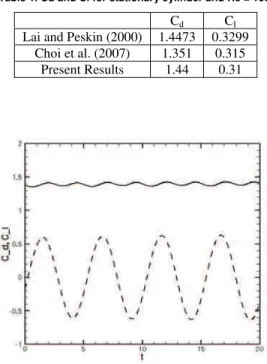
The results of the simulations of flow over a stationary circular cylinder were compared with the numerical results by Peskin (2000) and Choi et al. (2007). The simulations were performed for Re = 100 and a comparison is given in Table 1. The drag and lift coefficients Cd and Cl are shown in Fig. 2. The results given by this
study show some differences when compared with the results by Choi et al. (2007), but are in good agreement with results given by Lai and Peskin (2000).
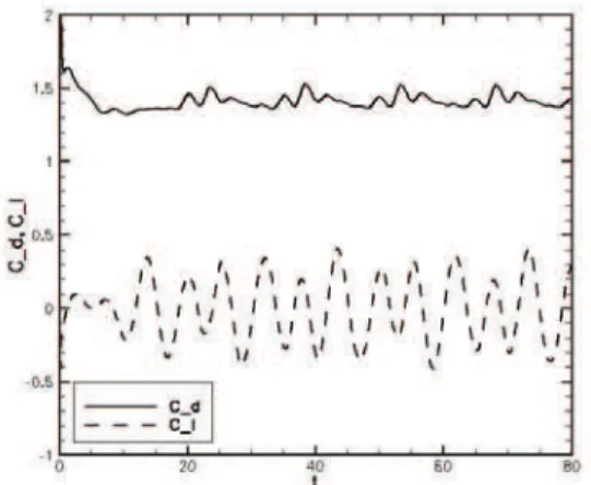
Another simulation with Re = 200 was performed in order to compare the results with the ones by Liu et al. (1998). The drag and lift coefficients are shown in Fig. 3. Values of Cd = 1.39 and Cl =
0.63 were obtained, and are in good agreement with the ones by Liu et al. (1998), which were between 1.17 and 1.58 for Cd, and between
0.50 and 0.69 for Cl.
Figure 2. Cl and Cd for stationary cylinder with Re = 100.
Table 1. Cd and Cl for stationary cylinder and Re = 100.
Cd Cl
Lai and Peskin (2000) 1.4473 0.3299 Choi et al. (2007) 1.351 0.315
Present Results 1.44 0.31
Figure 3. Cd and Cl for stationary cylinder and Re = 200.
Cylinder oscillating in the flow direction
In order to verify the implemented code with cylinder oscillations in the flow direction, initially, two simulations were performed: one with an oscillating cylinder and another with a stationary cylinder and an oscillating inflow velocity. The oscillation amplitude for the cylinder was A = 0.20, the frequency was F = 0.9 and the Reynolds number for these simulations was Re = 185. The vorticity contours obtained with each simulation at a given time are shown in Fig. 4. It can be seen that the vorticity contours in both cases are analogous.
In order to compare the results obtained with the proposed method with other numerical results, some simulations with the same parameters used by Al-Mdallal et al. (2007) were performed. These simulations were carried out with an oscillation amplitude of A = 0.10 and Reynolds number Re = 200. Three different frequencies were tested: F = 0.55, F = 2.20 and F = 2.80. Figures 5 to 7 show the comparison of the lift coefficient Cl for each case,
respectively. In all cases, the results are in agreement with the results by Al-Mdallal et al. (2007).
Other numerical simulations were carried out with the same parameters adopted in the experiment by Griffin and Ramberg (1976). The oscillation amplitude was A = 0.20 and the Reynolds number used was Re = 190.
Figure 4. Vorticity contour for flow over a cylinder oscillating in the flow direction (left) and oscillatory inflow over a stationary cylinder (right).
Figure 5. Cl for the cylinder oscillating in the flow direction with A = 0.10, F =
0.55 and Re = 200. Results given by Al-Mdallal et al. (2007) (top) and present results (bottom).
When the cylinder oscillates with F = 2.00, a couple of vortices with the same sign is observed, as shown in Fig. 10.
Figure 6. Cl for the cylinder oscillating in the flow direction with A = 0.10, F =
2.20 and Re = 200. Results given by Al-Mdallal et al. (2007) (top) and present results (bottom).
Figure 7. Cl for the cylinder oscillating in the flow direction with A = 0.10, F =
2.80 and Re = 200. Results given by Al-Mdallal et al. (2007) (top) and present results (bottom).
Figure 8. Vorticity contours for the cylinder oscillating in the flow direction with A = 0.20, F = 0.50 and Re = 190.
Figure 9. Vorticity contours for the cylinder oscillating in the flow direction with A = 0.20, F = 1.50 and Re = 190.
Figure 10. Vorticity contours for the cylinder oscillating in the flow direction with A = 0.20, F = 2.00 and Re = 190.
Figure 11. Vorticity contours for the cylinder oscillating in the flow direction with A = 0.20, F = 3.00 and Re = 190.
For frequency oscillation F = 3.00, a complex vortex shedding can be observed, as shown by vorticity contours in Fig. 11. Some small vortices appear at the top and lower parts of the cylinder.
It was possible to capture the lock-in phenomenon in cases with F = 1.50 and F = 2.00.
For F = 0.50 and F = 3.00, the lock-in phenomenon does not occur, and the streamwise is composed of five vortices. In Fig. 11, five vortices were considered, instead of eight, as the vortices with the same signal are coalescent.
Cylinder oscillating in the normal flow direction
The results given by the simulations of flow over a cylinder oscillating in the normal flow direction were compared with the numerical results given by Nobari and Naderan (2006). The oscillation frequencies tested were F = 0.60 and F = 1.05, with amplitude oscillation A = 0.20 and A = 0.40. The Reynolds number was Re = 100.
The curves of drag and lift coefficients when the cylinder oscillates with frequency F = 0.60 and amplitude A = 0.20 are shown in Fig. 12. The lock-in phenomenon does not occur in this case, as observed by Nobari and Naderan (2006). According to them, if the lock-in phenomenon does not occur, there is an intermittent vortex shedding due to the double-frequency influence. Figure 13 shows the vortex shedding for A = 0.20 and F = 0.60. Figure 14 shows the drag and lift coefficients for A = 0.20 and F = 1.05. The vortex shedding can be observed in Fig. 15. For these values, the lock-in phenomenon occurs, forming a regular vortex shedding.
Figure12. Cd and Cl for the cylinder oscillating in the normal flow direction
with A = 0.20, F = 0.60 and Re = 100.
Figure 13. Vorticity contours for the cylinder oscillating in the normal flow direction with A = 0.20, F = 0.60 and Re = 100.
Figure 14. Cd and Cl for the cylinder oscillating in the normal flow direction
with A = 0.20, F = 1.05 and Re = 100.
Figure 15. Vorticity contours for the cylinder oscillating in the normal flow direction with A = 0.20, F = 1.05 and Re = 100.
Figure 16. Cd and Cl for the cylinder oscillating in the normal flow direction
with A = 0.40, F = 0.60 and Re = 100.
When A = 0.40 and F = 0.60, the lock-in phenomenon does not occur. Figure 16 shows the drag and lift coefficients, and the vortex shedding can be seen in Fig. 17.
The results for Cd and Cl when A = 0.40 and F = 1.05 are given
in Fig. 18. Figure 19 shows the vortex shedding for this case. Here, the lock-in phenomenon can be observed, with a regular vortex shedding. A comparison between Cd and Cl can be observed in
The drag coefficient obtained, for an oscillation amplitude of A = 0.40, frequency of F = 1.05, and the present code was Cd = 2.309, which
is in agreement with Nobari and Naderan (2006), Cd = 2.31.
Cylinder with angular oscillation
For the verification of the flow over the cylinder with angular oscillations, the results were compared with the numerical results given by Baek and Sung (1998). Here, the amplitude oscillation is defined as a maximum rotation angle, α. The Reynolds Number was Re = 110.
The first simulation was performed with α = 15º of maximum rotation angle and two different frequency values: F = 0.15 and F = 0.17. The lift coefficient for F = 0.15 is shown in Fig. 20. It can be observed that there is a sign change in Cl. According to Baek and
Sung (1998), the frequency of F = 0.15 is a critical point (i.e., the lock-in phenomenon occurs).
A comparison between the lift coefficients obtained with the proposed code and the results given by Baek and Sung (1998) is shown in Table 3.
A second test was performed for rotation angle α = 30º. The lift coefficient comparison for the results obtained with the present code and the results given by Baek and Sung (1998) is shown in Table 4.
The last comparisons were carried out with an oscillation angle
α = 60º with three different frequency values: F = 0.14, F = 0.17 and F = 0.20. The results for lift coefficients obtained with the present code and the results by Baek and Sung (1998) are shown in Table 5. Figure 17. Vorticity contours for the cylinder oscillating in the normal flow
direction with A = 0.40, F = 0.60 and Re = 100.
Figure 18. Cd and Cl for the cylinder oscillating in the normal flow direction
with A = 0.40, F = 1.05 and Re = 100.
Figure 20. Cl for rotating cylinder, α = 15º and F = 0.15.
Table 3. Cl for rotating cylinder, α = 15º.
F = 0.15 F = 0.17 Baek and Sung (1998) 0.5 0.75
Present Results 0.60 0.70
Table 4 . Cl for rotating cylinder, α = 30º.
F = 0.14 F = 0.17 F = 0.20 Baek and Sung (1998) 0.75 1.10 0.48
Present Results 0.86 1.04 0.90
Table 5 . Cl for rotating cylinder, α = 60º.
F = 0.14 F = 0.17 F = 0.20 Baek and Sung (1998) 1.40 1.60 0.81
Present Results 1.10 1.63 1.40
Figure 19. Vorticity contours for the cylinder oscillating in the normal flow direction with A = 0.40, F = 1.05 and Re = 100.
Table 2. Cl comparison for amplitude oscillation A = 0.20.
In the simulations for the flow over cylinders with angular oscillation, the results were in agreement with Baek and Sung (1998). The only discrepancy was observed for frequency F = 0.20. F = 0.60 F = 1.05
Conclusions
The aim of this study was to propose an Immersed Boundary Method to simulate the flow over rigid bodies. A rigid body can be stationary or moving in the flow field. A circular cylinder was taken as a rigid body for verification and validation. Four different cases were simulated: flow over a steady cylinder, flow over an oscillating cylinder in the same direction of the flow, cylinder oscillating in the normal flow direction and flow over a cylinder with angular oscillation. The numerical results were compared to numerical and experimental results.
The drag and lift coefficients and vorticity contour plots were used for comparisons. With the vorticity contour plots, the vortex shedding could be analyzed. The lock-in phenomenon was used for verification and validation of the proposed code with a moving rigid body. The influence of the changes in frequency and amplitude oscillation on the lock-in phenomenon was also studied. The results were in good agreement with the numerical and experimental results.
In all simulations the CFL number was CFL = 0.2. The results have shown that the proposed method is suitable for numerical simulations over rigid bodies, stationary or not. The extension of the present code for simulations over bodies with different configurations and/or for three dimensional simulations is straightforward.
References
Al-Mdallal, Q., Lawrence, M. and Kocabiyik, S., 2007, “Forced streamwise oscillations of a circular cylinder: Locked-on modes and resulting fluid forces”, Journal of Fluids and Structures, Vol. 23, pp. 681-701.
Baek, S.J. and Sung, H.J., 1998, “Numerical simulation of the flow behind a rotary oscillating circular cylinder”, Physics of Fluids, Vol. 10, pp. 869-876.
Balaras, E., 2004, “Modeling complex boundaries using an external force field on fixed Cartesian grids in large-eddy simulations”,
Computers & Fluids, Vol. 33, pp. 375-404.
Burrowes, M., Farina, C., 2005, “On the isochronous pendulum of Christian Huygens”, Revista Brasileira do Ensino de Física, Vol. 27, No. 2, pp. 175-179.
Choi et al., 2007, “An Immersed Boundary Method for complex incompressible flows”, Journal of Computational Physics, Vol. 36, pp. 757-784.
Choi, S. and Choi, H.A., 2002, “Modification of the Aerodynamic Characteristics of Bluff Bodies Using Fluidic Actuators”, Physics of Fluids, Vol. 14, pp. 2767-2777.
Gosdtein, D., Handler, R. and Sirovich, L., 1993, “Modelling no-slip flow boundary with an external force field”, Journal of Computational Physics, Vol. 105, pp. 354-366.
Griffin, O.M. and Ramberg, S.M., 1976, “Vortex shedding from a cylinder vibrating in-line with an incident uniform flow”, Journal of Fluid Mechanics, Vol. 75, pp. 257-271.
Kloker, M., Konzelman, U. and Fasel, H.F., 1993, “Outflow boundary conditions for spatial Navier-Stokes simulations of transition boundary layers”, AIAA Journal, Vol. 31, pp. 620-628.
Lai, M.C., Peskin, C.S., 2000, “An Immersed Boundary Method with Formal Second-Order Accuracy and Reduced Numerical Viscosity”,
Journal of Computational Physics, Vol. 160. pp. 705-719.
Lima e Silva, A.L.F., Neto, A.S., Damasceno, J.R., 2003, “Numerical simulation of two dimensional flows over a circular
cylinder using the immersed boundary method”, Journal of
Computational Physics, Vol. 189, pp. 351-370.
Linnick, M.N. and Fasel, H.F., 2003, “A high-order immersed boundary method for unsteady incompressible flow calculations”, Aerospace Sciences Meeting and Exhibit – AIAA – 2003 – 1124, Wiley: Chichester, pp. 289-309.
Linnick, M.N., 1999, “Investigation of actuators for use in active flow control”, MS.c. Dissertation, University of Arizona, EUA.
Liu, C., Zhang, X., Sung, H.C., 1998, “An Immersed Boundary Method with Formal Second-Order Accuracy and Reduced Numerical Viscosity”, Journal of Computational Physics, Vol. 139. pp. 35-57.
Mohd-Yusof, J., 1997, “Combined immersed boundary B-spline methods for simulation of flow in complex geometries”, Annual Research Briefs – Center Turbulent Research, Vol. 105, pp. 317-324.
Nobari, M.R.H., Naderan, H., 2006, “A numerical study of flow past a cylinder with cross flow and in line oscillation”, Journal of Computational Physics, Vol. 35, pp. 393-415.
Peskin, C.S., 1972, “Flow patterns around heart valves: a numerical method”, Journal of Computational Physics, Vol. 10, pp. 252-271. Peskin, C.S., 1977, “Numerical Analysis of Blood Flow in the Heart”, Journal of Computational Physics, Vol. 25, pp. 220-252.
Peskin, C.S., 2002, “The Immersed Boundary Method”, Acta Numerica, pp 479-517.
Saiki, E.M. and Biringen, S., 1996, “Numerical Simulation of a Cylinder in Uniform Flow: Application in a Virtual Boundary Method”,
Journal of Computational Physics, Vol. 36, pp. 450-465.
Souza, L.F., Mendonça, M.T. and Medeiros, M.A.F., 2005, “The advantages of using high-order finite differences schemes in laminar-turbulent transitions studies”, International Journal for Numerical Methods in Fluids, Vol. 48, pp 565-592.