Numerical Simulation of Free Surface in the Case of Plane Turbulent Wall Jets in Shallow Tailwater

* Corresponding author E-mail: javanmi@gmail.com 189

Numerical Simulation of Free Surface in the Case of Plane Turbulent

Wall Jets in Shallow Tailwater

Javan, M. 1*, Eghbalzadeh, A. 2 and Montazeri Namin, M.3

1

Assistant Professor, Department of Civil Engineering, Faculty of Engineering, Razi University, Kermanshah, Iran.

2

Assistant Professor, Water and Wastewater Research Center, Razi University, Kermanshah, Iran.

3

Assistant Professor, School of Civil Engineering, College of Engineering, University of Tehran, P.O.Box: 11155-4563, Tehran, Iran.

Received: 13 May 2012; Revised: 25 Nov. 2012; Accepted: 25 May 2013 ABSTRACT: Wall-jet flow is an important flow field in hydraulic engineering, and its applications include flow from the bottom outlet of dams and sluice gates. In this paper, the plane turbulent wall jet in shallow tailwater is simulated by solving the Reynolds Averaged Navier-Stokes equations using the standard k turbulence closure model. This study aims to explore the ability of a time splitting method on a non-staggered grid in curvilinear coordinates for simulation of two-dimensional (2D) plane turbulent wall jets with finite tailwater depth. In the developed model, the kinematic free-surface boundary condition is solved simultaneously with the momentum and continuity equations, so that the water surface elevation can be obtained along with the velocity and pressure fields as part of the solution. 2D simulations are carried out for plane turbulent wall jets free surface in shallow tailwater. The comparison undertaken between numerical results and experimental measurements show that the numerical model can capture the velocity field and the drop in the water surface elevation at the gate with reasonable accuracy.

Keywords: Numerical Simulation, Free Surface, Shallow Tailwater, Turbulent Flow,

Water Jets.

INTRODUCTION

A plane wall-jet is obtained by injecting fluid parallel to a wall in such a way that the velocity of the fluid, over some distance from the wall, supersedes that of the ambient flow (Launder and Rodi, 1981). The structure of a turbulent wall-jet can be described as being composed of two canonical shear layers of different type. The inner shear layer, reaching from the wall out

190 For a plane turbulent wall (or bed) jet discharged into relatively deep tailwater, if the shear stress on the bed is neglected, it has been generally assumed, as in the case of a plane free jet, that the momentum flux will be preserved (see for example, Rajaratnam, 1976). Turbulent plane wall jets in shallow tailwater have important applications in hydraulic engineering such as submerged sluice gates, other types of outlets, and submerged hydraulic jumps that flow field can be treated as wall jets (Wu & Rajaratnam, 1995). The plane wall jet model has been used to analyse a number of flows in hydraulic structures, where the tailwater depth might not even be very large (Ead and Rajaratnam, 2002).

Several laboratory experiments have been performed to study turbulent plane wall jets (Albertson et al., 1950; Goldschmidt & Eskinazi, 1966; Heskestad, 1965; Kotsovinos, 1975; Miller & Comings, 1957; Eriksson et al., 1998). Swean et al. (1989) studied the variation of momentum and volume fluxes as well as the growth of plane turbulent surface jets with limited depth of tailwater. Their results showed a momentum decay and a breakdown (or variation from that of jets in infinite ambient) in the velocity and length scales due to the jet confinement. Ead and Rajaratnam (1998, 2001) have shown that the decay of the momentum flux is significant even for relatively large tailwater over a distance of 300–900 slot widths. Ead and Rajaratnam (2002) studied plane turbulent wall jets with finite tailwater depth. The main objective of that study (Ead and Rajaratnam, 2002) was to show that, when the depth of tailwater is finite, the momentum flux of the forward flow in the wall jet decays appreciably with the distance from the nozzle. This decay is due to the entrainment of the return flow, which has negative momentum that requires a depression of the water surface near the gate housing the slot. For turbulent wall jets

in shallow tailwater, it has been shown theoretically and experimentally that the momentum flux in the forward flow region of the wall jet is not preserved and the depression in the water surface elevation at the gate is created to produce the required pressure gradient to drive the return flow above the wall jet, for the jet entrainment (Ead and Rajaratnam, 2002).

Field and laboratory experiments can provide valuable information on flow characteristics by measurements and flow visualization, but the cost to conduct these experiments is expensive. With the rapid development of numerical methods and advancements in computer technology, CFD has been widely used to study plane wall jets. Kechiche et al. (2004) used closure models called “low Reynolds number k models”, which are self-adapting ones using different damping functions, in order to explore the computed behaviour of a turbulent plane two-dimensional wall jets. Shojaeefard et al. (2007) compared low Reynolds number k and 2f turbulence closure models for simulating a turbulent plane two-dimensional wall jets. Khosronejad and Rennie (2010) simulated unconfined and confined 3D wall-jet flow with low-turbulence Reynolds number k and standard k turbulence closure models.

191 two-dimensional (2D) plane turbulent wall jets with finite tailwater depth is developed. In this model, the kinematic free-surface boundary condition is solved simultaneously with the momentum and continuity equations, so that the water surface elevation can be obtained along with the velocity and pressure fields as part of the solution. The non-staggered-grid method of Rhie and Chow couples the volume flux on the face of the cell to the Cartesian velocity components at the cell centre. In this way, both momentum and the continuity equations are enforced in the same control volume.

GOVERNING EQUATIONS

The flow field is determined by the following incompressible fluid Reynolds-averaged continuity and momentum equations. The equations are written here in a general form:

0    i i x u (1) j ij i j j i i x x x u u t u                1 (2)

where u_i(i1,2) are the velocity components;  is the pressure divided by fluid density;= fluid density. The turbulent stresses _ijare calculated with the standard

 

k turbulence model (Rodi, 1993), which employs the eddy viscosity relation:

k x u x u ij i j j i t

ij  

 3 2                With  _t c_ k2

(3)

where the turbulent kinetic energy,k, and its dissipation rate,, determining the eddy

viscosity, t , are obtained from the following equations:    _{ }                   G x k x x k u t k j k t j j j (4)





k c G c x x x u t _j t j j j           2 1                     (5)

HereG_t





u_i x_j

 

 u_j x_i





u_i x_j



is the production ofk. The standard values of the model coefficients are used:

. 3 . 1 , 0 . 1 , 92 . 1 , 44 . 1 , 09 .

0 ₁ ₂  

 _{  }

 c c  and

c _k

Governing equations are transformed into curvilinear coordinates in the strong-conservation-law form: 0    m m U  (6) 0 1        m im i F t u J  (7)

where the flux is:

n i mn t i m i m im u GG x J u U F          

 1

(8)

where J1is the inverse of Jacobian or volume of the cell; Umis the volume flux

(contravariant velocity byJ1) normal to the surface of constant_m; and GGmnis called the “mesh skewness tensor”. These quantities are expressed as:

j j m m u x J U    1 

(9)             j i x J  det 1 (10) j n j m mn x x J GG      1  

192

NUMERICAL METHOD

The non-staggered-grid layout is employed. The pressure and the Cartesian velocity components are defined at the centre and the volume fluxes are defined at the mid-point of their corresponding faces of the control volume in the computational space (Figure 1). An explicit time-advancement scheme is used for pressure term, convection and diffusion terms. The discretized equations are: 0 1     m n m U  (12)

 

n

i n i n i n i n i D R C t u u

J   

 



1 1 _{ (13)}

n n n k n k n n G D C t k k

J    

 



1 1 ₍₁₄₎

            _          n n n n n n n n n k c G c D C t J          2 1 2 1 1 1 (15)

where  mrepresents discrete finite

difference operators in the computational space; superscripts represent the time step;

C represents the convective terms; R_i is the discrete operator for the pressure gradient terms; and D is discrete operators representing viscous terms. They are:

m m m m k m i m i U C k U C u U C      _          ) ( , ) ( , ) ( (16)              i m m i x J R 

 1 (17)

                                 n mn e t m n mn k t m k n mn t m i GG D GG D GG D             , , (18)

Except for the convective terms, all the spatial derivatives are approximated with second-order central differences. The C_i convective terms are discretized using Second-order Upwind (SOU) which calculates the face value from the nodal values using a quadratic upwind interpolation, CkandCare discretized using

Power-law Scheme (POW). The application of the fractional step method (Kim & Moin, 1985) to Eq. (13) leads to the following predictor-corrector solution procedure:

193 1. Predictor

 

) ( 1 * n i n i n i n i

i C R D

J t u

u   _    (19)

2. Corrector

 







   _  i i n i R J t u

u 1 * ₁ (20)

The variableui* is called the “intermediate

velocity” which is not constrained by continuity. The variable is related to

1  n  by:   n1  n 

(21)

The variable  is obtained by solving the pressure correction Poisson equation which is derived directly by the following procedure. First, the equation is derived for the volume flux U_mn1. If the corrector step of the fractional step method (Eq. (20)) is applied to compute the Cartesian velocity components defined on a face of the control volume, it achieves:

face m i m face i face n i x t u u                   ) ( )

( 1 *

(22)

The above equation is different from Eq. (20), in that, instead of being written in the strong-conservation-law form, the pressure correct gradient is written in the chain-rule-conservation-law form. Combining (Eq. (22)) with Eq. (9), the following equation is obtained for the estimation of U_mn1:

             n mn m n

m U t GG

U

 

1

(23)

where U_mn1 and U_mare defined on the cell faces. U_m is obtained by the special

interpolation presented by Rhie and Chow (1983) as:                                 face n n face n n mn m

m U t GG

U     * * (24)

where



n _n



is firstly computed at the

cell centre and U_m* and



n _n



are computed onto the cell faces by interpolating

*

i

u and



n _n



, respectively. By substituting Eq. (23) into Eq. (12), the pressure correct Poisson equation is obtained as: m m n mn m U t GG                    1 (25)

The above derivation results in a pressure correct Poisson equation whose coefficients only consist of the mess skewness tensor mn

GG . This elliptic equation is solved using a block tri-diagonal algebraic system of the equations.

BOUNDARY CONDITION

194 normal gradients of all dependent variables are set equal to zero. Since one boundary of the domain is located at the free surface, the moving-grid (Lagrangian) method was used for simulating the free surface (Namin et al., 2001; Javan et al., 2007). At this free boundary, the kinematic and dynamic conditions are imposed.

COMPUTATIONAL GRID AND

MODEL SETUP

In this study, two experiments investigated by Ead and Rajaratnam (2002) are simulated to evaluate the numerical model. The model grid used (a vertical sigma-coordinate and horizontal curvilinear none-orthogonal system) makes it possible to resolve the issue of the plane turbulent wall jets free surface in shallow tailwater. In these simulations, the grid system is upgraded after estimating the free surface elevation in each time step. A simple approach is followed where a certain number of grids (usually grids between bed and inlet jet thickness) above the bed is fixed uniformly. The grid numbers at inlet jet thickness are not affected by free surface level change. The rest of the grids are moved non-uniformly to a vertical distance according to free surface level change calculated from the free surface boundary conditions.

For the numerical simulation of the first series of experiments (series A) conducted by Ead and Rajaratnam (2002), a 7.5 m long computational domain is employed in order

to avoid reflections from the outlet. In the upstream and downstream regions of the channel (0x3m and 3x7.5m), the domain contains 301 uniform and 200 non-uniform grids in the x direction, respectively. In the y-direction, the calculations contain 5 uniform and 46 non-uniform grids in the inlet jet thickness and above it, respectively. A time step of 0.001 second is adopted. Another series of experiments (series B) are conducted mainly to measure the drop in the water surface elevation at the gate. In the upstream and downstream regions of the channel (0x1mand1x2.0 m), the domain contains 101 uniform and 40 non-uniform grids in the x direction, respectively. In the y-direction, the domain contains 5 uniform and 26 non-uniform grids in the inlet jet thickness and above it, respectively. A time step of 0.0005 second is adopted.

RESULTS AND DISCUSSION

Consider a plane turbulent wall jet of thickness b₀ with a flow rate per unit width of Q0 entering a rectangular channel, tangentially on its bed as shown in Figure 2. Let U₀be the velocity of the jet at the inlet slot (or nozzle). The outlet water level is adjusted so that the tailwater depth, y_t, is large enough to make the water level immediately downstream of the gate (housing the slot) horizontal (see Figure 2).

195 In this study, the model is first used to simulate the flow field and free surface introduced by the first experiment of series A conducted by Ead and Rajaratnam (2002). Table 1 shows the primary details of the first experiment of series A (Experiment 1).

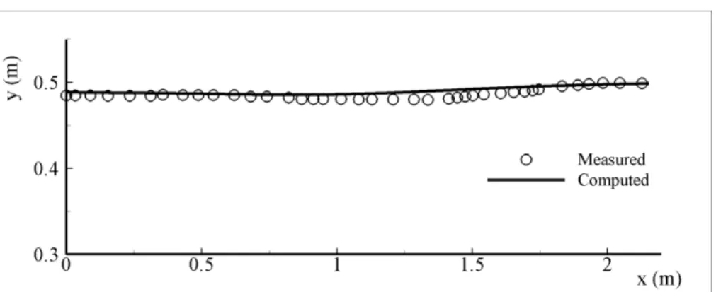
Water-surface elevations and velocity fields obtained using the numerical model are compared with the experimental measurements of the first experiment of series A conducted by Ead and Rajaratnam (2002) in Figures 3 and 4. Figure 4 shows the velocity profiles in the forward flows at several sections with x varying from 12 to 140 cm; y is the distance above the bed. As shown in Figures 3 and 4, the agreement between measured data and numerical results is reasonably good. The mean relative error between the experimental and numerical results of water-surface elevations is about 0.85% as shown in Figure 3. Figure 5 presents the relative errors of the maximum velocities in different sections. At the upstream sections, as seen in Figure 5, the relative error of numerical model predictions are less than 5%, but further downstream in section x=140 cm, this increases up to about 19%. As noticed in Figure 3, the water surface in the vicinity of the gate is approximately horizontal. The depression in the water surface elevation at the gate is also shown in Figure 3.

The primary details for one experiment of the series B (Experiment 2) are shown in

Table 1. The measured depression in the water surface elevation at the gate, from that of the tailwater is 4 cm at Experiment 2. Figure 6 shows simulated free surface profiles and streamline pattern for Experiment 2.

The surface eddy, the depression in the water surface elevation at the gate and the rise in the region with x varying from 0.115 to 1.12 m can be seen in Figure 6. The depression simulated in the water:

Surface elevation at the gate, from that of the tailwater is 4.8 cm (see Figure 6), which is in good agreement with the measurements undertaken by Ead and Rajaratnam (2002). It appears that the depression in the water surface elevation at the gate is created to produce the required pressure gradient to drive the return flow above the wall jet, for the jet entrainment (Ead and Rajaratnam, 2002).

CONCLUSIONS

Details of a numerical model to simulate two-dimensional (2D) plane turbulent wall jets with finite tailwater depth using the full vertical momentum equations are presented. The numerical model is developed on a non-staggered grid in curvilinear coordinates. Using this model, water elevation, and pressure and velocity fields can be simulated simultaneously.

196

Fig. 4. Comparison of simulated velocity field with the experimental measurements of Ead and Rajaratnam (2002) (Experiment 1).

Fig. 5. The relative errors of the maximum velocities in different sections.

Table 1. Primary detail of two experiments of series A and B conducted by Ead and Rajaratnam (2002).

Experiment b₀

 

mm W

 

mm U₀ms F₀ y_t



mm



R

1 10 446 2.5 8.0 500 25000

2 10 446 2.5 8.0 150 25000

197

Fig. 6. Simulated free surface profiles and streamline pattern (Experiment 2).

Since the vertical momentum equation is treated in the same way as the horizontal momentum equation, the model can be used to predict free surface flows. Because both the flow pattern and the water elevation are considerable significance in 2D plane turbulent wall jets with finite tailwater depth, two numerical simulations are performed to verify the simulated flow pattern and water elevation. The comparison of the numerical results with the experimental measurements show that the numerical model can capture the flow pattern, typical velocity distribution and the drop in the water surface elevation at the gate with reasonable accuracy for 2D plane turbulent wall jets with finite tailwater depth. The numerical model presented here is practical and easy to apply, because the solution of flow fields at a time step is obtained without iteration, and only the values ofy,x and t affect the accuracy of the free-surface and flow pattern simulated. Although the model presented in this paper is for two-dimensional flows in the vertical plane, its application can be extended to model three-dimensional flows.

REFERENCES

Albertson, M.L., Dai, Y.B., Jenson, R.A. and Rouse, H. (1950). “Diffusion of submerged jets”,

Transactions of the American Society of Civil Engineer, 115, 639–664.

Ead, S.A. and Rajaratnam, N. (1998). “Double-leaf gate for energy dissipation below regulators”,

Journal of Hydraulic Engineering, 124(11), 1134–1145.

Ead, S.A. and Rajaratnam, N. (2001). “Plane turbulent surface jets in shallow tailwater”,

Journal of Fluids Engineering, 123, 121–127. Ead, S.A. and Rajaratnam, N. (2002). “Plane

turbulent wall jets in shallow tailwater”, Journal of Engineering Mechanics, 128(2), 143-155. Eriksson, J.G., Karlsson, R.I. and Persson, J. (1998).

“An experimental study of a two-dimensional plane turbulent wall jet”, Experiments in Fluids, 25(1), 50–60.

Goldschmidt, V. and Eskinazi, S. (1966). “Two phase turbulent flow in a plane jet”, Transactions ASME, Series E, Journal of Applied Mechanics, 33(4), 735–747.

Heskestad, G. (1965). “Hot wire measurements in a plane turbulent jet”, Transactions ASME, Series E, Journal of Applied Mechanics, 32(4), 721–734. Javan, M., Montazeri Namin, M. and Salehi Neyshabouri, S.A.A. (2007). “A time-splitting method on a non-staggered grid in curvilinear coordinates for implicit simulation of non-hydrostatic free-surface flows”, Canadian Journal of Civil Engineering, 34(1), 99-106.

Kechiche, K., Mhiri, H., Palec, G.L. and Philippe, B. (2004) “Application of low reynolds number

 

k turbulence models to the study of turbulent wall jets”, International Journal of Thermal Sciences, 43, 201–211.

198

turbulence models”, Canadian Journal of Civil Engineering, 37(4), 576–587.

Kim, J. and Moin, P. (1985). “Application of a fractional-step method to incompressible navier-stokes equations”, Journal of Computational Physics, 59, 308-323.

Kotsovinos, N.E. (1975). “A study of the entrainment and turbulence in a plane turbulent jet”, California Institute of Technology, Rep. KH R-32, W. M. Keck Laboratory of Hydrology and Water Resources, Pasadena, California.

Launder, B.E. and Rodi, W. (1981). “The turbulent wall jet”, Progress in Aerospace Sciences, 19, 81– 128.

Miller, D.R. and Comings, E.W. (1957). “Static pressure distribution in the free turbulent jet”,

Journal of Fluid Mechanics, 3(1), 1–16.

Montazeri Namin, M., Lin, B. and Falconer, R.A. (2001). “An implicit numerical algorithm for solving non-hydrostatic free-surface flow problems”, International Journal of Numerical Methods in Fluids, 35, 341-356.

Rajaratnam, N. (1976). Turbulent jets, Elsevier, Amsterdam, the Netherlands, 304p.

Rhie, C.M. and Chow, W.L. (1983). “Numerical study of the turbulent flow past an airfoil with trailing edge separation”, AIAA Journal, 21, 1525-1532.

Rodi, W. (1993). Turbulence models and their applications in hydraulics - A state-of-arts review, IAHR Monograph, Balkema, Rotterdam, The Netherlands.

Shojaeefard, M.H., Goudarzi, K. and Jahromi, H.G. (2007) “Numerical simulation of 2D turbidity currents and wall jet”, American Journal of Applied Sciences, 4(11), 880-886.

Swean, T.F.Jr., Ramberg, S.E., Plesniak, M.W. and Stewart, M.B. (1989). “Turbulent surface jet in channel of limited depth”, Journal of Hydraulic Engineering, 115(12), 1587–1606.

Wu, S. and Rajaratnam, N. (1995). “Free jumps, submerged jumps and wall jets”, Journal of Hydraulic Research, 33(2), 197–212.