NONLINEAR
H
∞CONTROL FOR UNDERACTUATED MANIPULATORS
WITH ROBUSTNESS TESTS
Adriano A. G. Siqueira
∗Marco Henrique Terra
∗∗Electrical Engineering Department, University of S˜ao Paulo - S˜ao Carlos, SP, Brazil
ABSTRACT
In this paper, the model-based robotic control problem with disturbance attenuation (or robotic H∞ control problem), presented in Chenet all (1994), is extended to underactuated manipulators. The dynamic coupling between the links is used to control all manipulator’s free joints. A global explicit solution is found solving a minimax Bellman-Isaacs equation, generated via dif-ferential game theory. Experimental results, obtained from UArm II manipulator, considering fully actuated and underactuated configurations, are presented.
KEYWORDS: Robust control, nonlinearH∞control,
un-deractuated manipulators.
RESUMO
Neste artigo, o problema de controle rob´otico baseado em modelo com atenua¸c˜ao de dist´urbios (ou problema de controle H∞ rob´otico), apresentado em Chen et all (1994), ´e estendido para robˆos manipuladores subatu-ados. O acoplamento dinˆamico entre os elos ´e usado para controlar todas as juntas livres do manipulador. Uma solu¸c˜ao expl´ıcita global ´e encontrada resolvendo um problema minimax definido atrav´es de uma equa¸c˜ao de Bellman-Isaacs gerada pela teoria dos jogos. Resul-tados experimentais, obtidos com o manipulador UArm II, considerando as configura¸c˜oes totalmente atuada e subatuada, s˜ao apresentados.
Artigo submetido em 31/10/01
1a. Revis˜ao em 22/01/03; 2a. Revis˜ao em 10/06/03 Aceito sob recomenda¸c˜ao do Ed. Assoc. Prof. Liu Hsu
PALAVRAS-CHAVE: Controle robusto, controleH∞ n˜ao
linear, manipuladores subatuados.
1
INTRODUCTION
Motion control of manipulators has been the objective of a great number of researches (Chenet all, 1994; Chen and Chang, 1997; Johansson, 1990; Postlethwaite and Bartoszewicz, 1998). Underactuated manipulators, with less actuator than degrees of freedom, are also of interest for many researchers (Arai, 1997; Arai and Tachi, 1991; Bergerman, 1996). The controllability for these mechan-ical systems and a control strategy were first established in Arai and Tachi (1991). First, all passive joints (with-out actuator) are controlled to theirs set-point, using the dynamic coupling. Then, with the passive joints locked, the active ones (with actuator) are controlled by themselves. In Bergerman (1996), three possibilities of selecting the joints to be controlled at every control phase are derived. One can select only passive joints, passive and active joints or only active joints.
The effort to control the generalized coordinates of the manipulator (fully actuated or underactuated) to follow a desired trajectory can be a hard task if parameters uncertainties and exogenous disturbances are present. Robust control with a nonlinearH∞ criterion (Chenet
H∞ control for nonlinear time-invariant systems has been widely discussed since the past decade (Isidori, 1992; van der Sachft, 1991; van der Schaft, 1992; Ball
et all, 1991; Lu and Doyle, 1991). The nonlinear H∞
control problem means that we need to find an L2 in-duced norm between input and output signals limited by a levelγ. In Lu (1996), these results are extended to time-varying systems with finite-time horizon.
A roboticH∞control problem, or a model-based robotic control problem with desired disturbance attenuation, is proposed in Chenet all (1994). A global explicit solu-tion for this problem, formulated as a minimax (leader-following) game, is developed using differential game theory (Basar and Oslder, 1982; Basar and Berhard, 1990). From this theory, one needs to solve a minimax Bellman-Isaacs equation, which after some rearrange it is redefined as a Hamilton-Jacobi equation found in Lu (1996). The result of Chen et all (1994) is a kind of feedback linearization with a nonlinear term introduced in the control acceleration. Some experimental results were obtained in Postlethwaite and Bartoszewicz (1998) using a similar approach.
The formulation presented in Chenet all (1994) is re-sumed here as a background to the main results of this paper: the extension of the roboticH∞control problem for underactuated manipulators and the application of this methodology in the experimental robot manipulator UArm II, a three link planar manipulator with revolute joints, that can be configured as fully actuated or un-deractuated.
This paper is organized as follows. In Section 2, the robotic H∞ control problem is formulated based on
Chen et all (1994). In Section 3, this problem is
ex-tended to the underactuated case. In Section 4, the solution presented in Chen et all (1994), for this H∞ control problem, is described. In Section 5, experimen-tal results obtained from the UArm II are presented. In Section 6, the conclusions are presented.
This paper was previously presented in the International Workshop on Underwater Robotics for Sea Exploitation and Environmental Monitoring, held on October 2001 in Rio de Janeiro and organized by Professor Liu Hsu of Federal University of Rio de Janeiro.
2
ROBOTIC H
∞CONTROL PROBLEM
In this section, theH∞control problem is formulated for a manipulator where the disturbances are derived from parametric uncertainties and exogenous inputs, follow-ing the line defined in Chenet all (1994).
The dynamic equations of a manipulator can be found by the Lagrange theory as
τ=M(q) ¨q+C(q,q˙) ˙q+F( ˙q) +G(q) (1)
where q ∈ ℜn are the joint positions, M(q) ∈ ℜn×n is
the symmetric positive definite inertia matrix,C(q,q˙)∈ ℜn×n is the Coriolis and centripetal matrix,F
0( ˙q)∈ ℜn are the frictional torques, G(q) ∈ ℜn are the
gravita-tional torques andτ ∈ ℜn are the applied torques. The
parametric uncertainties can be introduced by dividing the parameter matrices M(q), C(q,q˙), F( ˙q), and G(q) into a nominal and a perturbed part
M(q) =M0(q) + ∆M(q) C(q,q˙) =C0(q,q˙) + ∆C(q,q˙) F( ˙q) =F0( ˙q) + ∆F( ˙q) G(q) =G0(q) + ∆G(q)
whereM0(q),C0(q,q˙),F0( ˙q), andG0(q) are the nominal matrices and ∆M(q), ∆C(q,q˙), ∆F( ˙q), and ∆G(q) are the parametric uncertainties. Exogenous inputs,w, can also be introduced, and (1) can be rewritten as
τ+δ=M0(q) ¨q+C0(q,q˙) ˙q+F0( ˙q) +G0(q) (2)
with
δ=−(∆M(q) ¨q+ ∆C(q,q˙) ˙q+ ∆F( ˙q) + ∆G(q)−w).
The state tracking error is defined as
˜
x=
˙
q−q˙d
q−qd
=
˙˜
q
˜
q
(3)
where qd and ˙qd ∈ ℜn are the desired reference
trajec-tory and the corresponding velocity, respectively. The variables qd, ˙qd, and ¨qd (desired acceleration), are
as-sumed to be within the physical and kinematics limits of the control object. The dynamic equation for the state tracking error is given from (2) and (3) as
˙˜
x=A(q,q˙) ˜x+B0 q,q,˙ q¨d,q˙d+BM0−1(q)τ+ BM0−1(q)δ (4)
where
A(q,q˙) =
−M0−1(q)C0(q,q˙) 0
In 0
B0(q,q,˙q¨d,q˙d) =
−q¨d
−M0−1(q)(F0( ˙qt) +G0(q) +C0(q,q) ˙˙qd)
0
B=
In
0
In order to represent this equation in a canonical form, a control input variableushould be defined. Using the following state-space transformation of ˜x (Chen et all, 1994; Johansson, 1990)
˜
z=
˜
z1 ˜
z2
=T0x˜=
T11 T12
0 I
˙˜
q
˜
q
(5)
and selecting the control input as
u=
M0(q) C0(q,q˙)
˙˜
z1 ˜
z1
=M0(q)T1x˙˜+C0(q,q˙)T1x˜
(6)
whereT11,T12 ∈ ℜn×n are constant matrices to be de-termined later andT1 = [T11 T12], the dynamic equa-tion of the state tracking error (4) can be rewritten as
˙˜
x=AT(˜x, t) ˜x+BT(˜x, t)u+BT(˜x, t)d (7)
where
AT(˜x, t) =T0−1
−M0−1(q)C0(q,q˙) 0 T−1
11 −T− 1 11 T12
T0
BT(˜x, t) =T0−1
M−1 0 (q)
0
d=M0(q)T11M0−1(q)δ.
The control input (6) is a selective applied torque, since it affects the kinetic energy only. It is not necessary to optimize the gravitation-dependent torques during the motion (Johansson, 1990). The relation between the applied torques and the control input is given by
τ =M0(q) ¨q+C0(q) ˙q+F0(q) +G0(q) (8)
where
¨
q= ¨qd−T11−1T12q˙˜−T11−1M0−1(q) C0(q)BTT0x˜−u. (9)
Equation (9) shows that a control acceleration, ¨qc, with
a nonlinear term, is generated by selecting the control input (6).
TheH∞control strategy aims to attenuate the effects of disturbance, solving the following performance criterion, with a desired attenuation levelγ
min
u(.)∈L
2 max
06=d(.)∈L
2
R∞
0 1 2x˜
T
(t)Qx˜(t) +1 2u
T
(t)Ru(t)
dt
R∞
0 1 2d
T(
t)d(t)
dt ≤γ
2
(10)
where Q and R are weighting matrices and ˜x(0) = 0. This performance criterion is actually theH∞ optimal disturbance attenuation problem for the model-based robotic control.
Remark (Chen et all, 1994): Formally, subject to the tracking error dynamics (7) a (full information)H ∞-control problem is to find a state feedback law such that
max 06=d(.)∈L2
kz(t)kL 2 kd(t)kL2
≤γ2
where
z(t) =
Q1/2x˜(t) R1/2u(t)
and||.||L2denotes the induced L2norm.
3
THE UNDERACTUATED CASE
Underactuated robot manipulators are mechanical sys-tems with less actuators than degrees of freedom. For this reason, the control of the passive joints (joint with-out actuator) is made considering the dynamic cou-pling between them and the active joints (with actu-ator). Here, we consider that the passive joints have brakes. The control strategy consists in controlling all the passive joints to reach the desired positions, applying torques in the active ones, and then turn on the brakes. After that, all the active joints control themselves.
Consider a manipulator with n joints, of whichnp are
passive andna are active joints. It is known (Arai and
Tachi, 1991) that no more than na joints of the
ma-nipulator can be controlled at every instant. Using this fact, we group thena joints being controlled in the
vec-torqc ∈ ℜna. The remaining joints are grouped in the
vector qr ∈ ℜn−na. There exist three possibilities of
forming the vectorqc (Bergerman, 1996)
1. qc contains only passive joints: whennp ≥na and
all other passive joints, if any, are kept locked.
2. qc contains passive and active joints: all other
pas-sive joints, if any, are kept locked.
3. qc contains active joints.
The control strategy is defined as follows: first, select
qc following the possibilities 1 or 2 (according to np),
until all passive joints have reached the desired position; second, selectqc following the possibility 3 and control
The dynamic equation (2) can be partitioned as τr τc + δr δc =
Mrr Mrc
Mcr Mcc
¨ qr ¨ qc +
Crr Crc
Ccr Ccc
˙ qr ˙ qc + Fr Fc + Gr Gc (11)
whereτrare the torques in the remaining joints andτc
are the torques in the controlled joints. For simplicity of notation, the index 0 representing the nominal system is eliminated from the equations.
For the control strategy 1, τc = 0 because there is no
torque in the passive joint. For the control strategy 2,
τc is defined asτc = [τac 0], whereτacis the torque in
the active joints being controlled. From the second line of (11)
τc+δc=Mcrq¨r+Mccq¨c+Ccrq˙r+Cccq˙c+Fc+Gc
we can isolate the controlled joint acceleration
¨
qc=−Mcc−1×
(Mcrq¨r+Ccrq˙r+Cccq˙c+Fc+Gc−τc−δc).(12)
Introducing a desired reference trajectory to the con-trolled joints (there is no desired reference to the un-controlled joints), (12) can be rewritten as
¨˜
qc =−Mcc−1Cccq˙˜c−q¨cd−Mcc−1Mcrq¨r−Mcc−1Ccrq˙r−
Mcc−1Cccq˙cd−Mcc−1Fc−Mcc−1Gc+Mcc−1τc+Mcc−1δc.
(13)
In the state-space form, selecting the state vector as
˜
xc=
˙
qc−q˙dc
qc−qdc
= ˙˜ qc ˜ qc , (14)
(13) can be defined as
˙˜
xc =A(q,q˙) ˜xc+B0 q,q,˙ q¨dc,q˙dc
+BM−1
cc τc+BMcc−1δc
(15)
where
A(q,q˙) =
−M−1
cc Ccc 0
In 0
B0
q,q,˙q¨dc,q˙
d c
=
−q¨d c−M
−1
cc Fcc+Gcc+Cccq˙dc+Ccrq˙r
−Mcc−1Mcrq¨r
0 B = In 0 .
Using a similar transformation like (5), the control input
uis selected as
u=
Mcc Ccc
˙˜ z1 ˜ z1
=MccT1x˙˜c+CccT1x˜c (16)
and the dynamic equation of the state tracking error (15) is redefined as
˙˜
xc =AT(˜xc, t) ˜xc+BT(˜xc, t)u+BT(˜xc, t)d (17)
where
AT(˜xc, t) =T0−1
−M−1
cc Ccc 0
T11−1 −T− 1 11 T12
T0
BT(˜xc, t) =T0−1
M−1
cc
0
d=Mcc(q)T11Mcc−1(q)δc.
Based on (16), the control acceleration can be given by
¨
qc = ¨qcd−T11−1T12q˙˜c−T11−1Mcc−1 CccBTT0x˜c−u. (18)
Equation (18) gives the necessary acceleration to the controlled joints follow the desired reference trajectory. The torques in the active joints can be computed using this control acceleration. One can use another form of representing the underactuated system, similar to (11), partitioning (2) as in Bergerman (1996)
τa 0 =
Mar Mac
Mur Muc
¨ qr ¨ qc + ba bu (19)
where the indexesaandurepresent active and unlocked passive joints, respectively, and b(q,q˙) = C(q,q˙) ˙q +
F( ˙q) +G(q) +δ. Factoring out the vector ¨qr in the
second line of (19) and substituting it in the first line, one obtains
τa= Mac−MarMur−1Mucq¨c+ba−MarMur−1bu.
Ifnp< na, the redundant control can also be considered.
In this case, the vector of controlled joints contains only the passive joints, qc = qu ∈ ℜnp, and the vector of remaining joints contains the active joints, qr = qa ∈
ℜna. The partitioned equation is defined as follows
τa 0 =
Maa Mau
Mua Muu
Factoring out the vector ¨qa in the second line, one
ob-tains
¨
qa =−Mua#(Muuq¨u+bu) + I−Mua#Muaz
whereM#
uais the pseudo-inverse of the (np×na) matrix
Muaandzis an arbitrary number. The applied torques
in the active joints can be computed as
τa= Mau−MaaMua#Muuq¨u+ba−MaaMur#bu+
Maa I−Mua#Muaz.
For the underactuated case, the performance criterion (10) is also used to attenuate disturbances.
4
ROBOTIC
H
∞CONTROL PROBLEM
SOLUTION
The solution of the roboticH∞control problem (10) can be explicitly found via differential game theory (Basar and Oslder, 1982; Basar and Berhard, 1990) with an appropriated Lyapunov function (Chen et all, 1994). In this section, a resume of the approach presented in (Chenet all (1994)) to solve this problem is presented.
The performance criterion (10) can be rewritten to de-fine the following minimax problem
min
u(.)∈L
2
max
06=d(.)∈L
2 Z ∞
0
1 2x˜
T
(t)Q˜x(t) +1 2u
T
(t)Ru(t)−1
2γ
2dT
(t)d(t)
dt≤0,
with ˜x(0) = 0. Defining the cost functional
J(˜x(t), u, d, t) = Z ∞
t
L(˜x(s), u(s), d(s))ds
with the Lagrangian
L(˜x, u, d) = 1 2x˜
T
(t)Qx˜(t) +1 2u
T
(t)Ru(t)−1
2γ
2dT
(t)d(t)
and introducing the Lyapunov function
V(˜x(t), t) = min
u(.)maxd(.) J(˜x(t), u, d, t)
the performance criterion (10) can be defined as
V (˜x(0),0) = min
u(.)maxd(.) J(˜x(0), u, d,0)≤0, x˜(0) = 0.
According to the differential game theory, the solution of this minimax (or leader-follower) problem is found if
there exists a continuously differentiable Lyapunov func-tionV(., .) that satisfies the following minimax Bellman-Isaacs equation
−∂V (˜x, t)
∂t = minu(.)maxd(.)
(
L(˜x, u, d) +
∂V (˜x, t)
∂x˜ T
˜
x
)
with terminal conditionV(˜x(∞),∞) = 0. Choosing a Lyapunov function of the form
V(˜x, t) =1 2x˜
TP(˜x, t) ˜x
whereP(˜x, t) is a positive definite symmetric matrix for all ˜xandt, the Bellman-Isaacs equation is then changed to the following Riccati equation
˙
P(˜x, t) +P(˜x, t)AT(˜x, t) +ATT(˜x, t)P(˜x, t)−
P(˜x, t)BT(˜x, t)
R−1− 1 γ2I
BT(˜x, t)P(˜x, t)+Q= 0.
(20)
The corresponding optimal control and the worst case disturbance are given, respectively, by
u∗=R−1BTT(˜x, t)P(˜x, t) ˜x
and
d∗= 1
γ2R −1BT
T (˜x, t)P(˜x, t) ˜x.
SelectingP(˜x, t) properly and using the skew symmetric matrixN(q,q˙) =C0(q,q˙) + (1/2) ˙M0(q,q˙) (Chenet all, 1994), the Riccati equation (20) can be simplified to an algebraic matrix equation. The matrix P(˜x, t) defined by Chenet all (1994) is given by
P(˜x, t) =T0T
M0(˜x, t) 0
0 K
T0
where K is a positive definite symmetric constant ma-trix. The simplified algebraic equation is given by
0 K
K 0
−T0TB
R−1− 1
γ2I
BTT0+Q= 0.
(21)
The optimal control and the worst case disturbance can be rewritten, respectively, as
u∗=R−1BTT
0x˜ (22)
and
d∗= 1
γ2R −1BTT
The terminal condition is satisfied for this matrixP(., .) (Chen et all, 1994). Then, to solve the robotic H∞ problem, we must find matricesK and T0 which solve the algebraic equation (21). Let the positive definite symmetric matrix Q be factorized as
Q=
QT
1Q1 Q12 QT12 QT2Q2
. (23)
The solution of (21) is given by
T0=
RT
1Q1 RT1Q2
0 I
(24)
and
K=1
2 Q
T
1Q2−QT2Q1−1 2 Q
T
12+Q12
with the conditions: K > 0 and R < γ2I. The matrix R1 is defined via Cholesky factorization
RT1R1=
R−1− 1
γ2I
−1
. (25)
Finally, the design algorithm can be outlined as follows
Step 1. Select a desired level of attenuation,γ >0.
Step 2. Select the weighting matrix R > 0 such that
λmax< γ2and the weighting matrixQas (23),
sat-isfyingK >0.
Step 3. Calculate the Cholesky factorization (25) and
T0 (24).
Step 4. Obtain the optimal control u* (22) and the optimal applied torque (8).
Considering the underactuated state tracking error (17),
P(˜x, t) can be chosen as
P(˜x, t) =TT
0
Mcc(˜x, t) 0
0 K
T0
since the matrix Mcc is symmetric positive definite.
Note thatNcc(q,q˙) =Ccc(q,q˙) + (1/2) ˙Mcc(q,q˙) is also
skew symmetric, then the design algorithm used to the totally actuated case can be applied to the underactu-ated case.
5
EXPERIMENTAL RESULTS
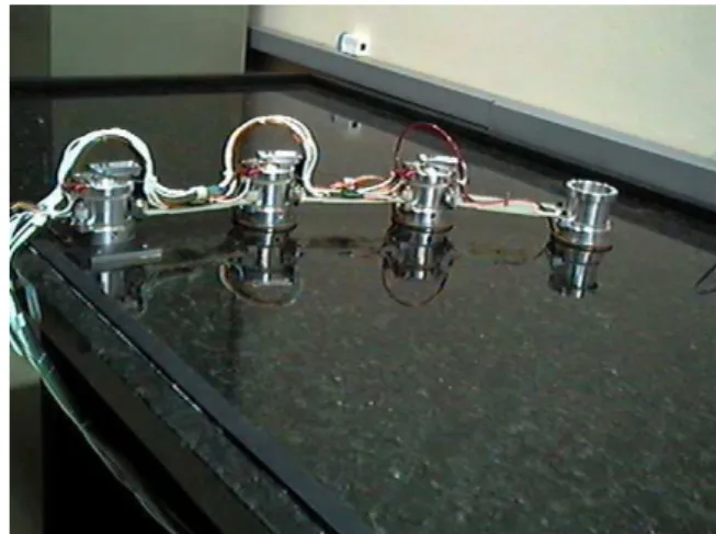
To validate the proposedH∞ control solution, it is ap-plied in our experimental underactuated manipulator
Figure 1: Underactuated Arm II.
UArm II (Underactuated Arm II), designed and built by H. Ben Brown, Jr. of Pittsburgh, PA, USA (Figure 1). This 3-link manipulator has special-purpose joints containing each one an actuator and a brake, so that they can act as active or passive joints. The manipula-tor configuration can be changed enabling or not the DC motor of each joint. Optical encoders with quadrature decoding are used to measure the joint positions. Joint velocities are obtained by numerical differentiation and filtering.
For interfacing between computer and manipulator, an input-output interface Servo-To-Go board is used. The board driver is accessed by dynamically linked libraries (dlls) compiled in the MatLab workspace by use of C++ program that containmex-functions.
A control environment was developed in a suitable way that all changes of configuration and the robot action can be done in a user friendly way. The UMCE (Under-actuated Manipulator Control Environment) is written in Matlab language and it is possible to see the real robot motion reproduced in its graphical interface (Figure 2). Simulation tests can also be done in this environment.
All possible configurations, according to active (A) and passive (P) joints location in the arm, are accepted: AAA, AAP, APA, PAA, APP, PAP, and PPA. For ex-ample, the configuration AAP means that joints 1 and 2 are active and joint 3 is passive.
The matrices M(q), C(q,q˙), and G(q) of (1) are eas-ily found via Lagrange theory for planar manipulators (Craig, 1989) (See Appendix A). However, the term
Figure 2: Graphical interface of the UMCE.
velocity-dependent frictional termF( ˙q) as
F( ˙q) =
f1q˙1 f2q˙2 f3q˙3
where the valuesf1,f2, andf3are selected after empir-ical tests. The manipulator’s kinematic and dynamic nominal parameters, which are used to calculate the nominal matricesM0(q),C0(q,q˙),F0( ˙q), andG0(q), are shown in Table I.
Table 1: Robot Parameters
Joint mi Ii li lci fi
(kg) (kg.m2) (m) (m) (kg.m2/s)
1 0.850 0.0075 0.203 0.096 0.45
2 0.850 0.0075 0.203 0.096 0.22
3 0.625 0.0060 0.203 0.077 0.22
The initial position for the experiment with configura-tion AAA is defined asq(0) = [0, 0, 0]oand the set-point
defined as q(T) = [20, 20, 20]o, where the vector T =
[T1 T2 T3] contains the time duration for the refer-ence trajectory for each joint. This vector is adequately selected taking into account the difference between the initial and final positions. The reference trajectory,qd,
is a fifth-degree polynomial trajectory.
The desired level of attenuation selected for the fully actuated case isγ= 3 with the following weighting ma-trices
Q1=I3, Q2= 2∗I3, Q12= 0, and R= 5∗I3.
Applying the design algorithm described in Section 4,
0 0.5 1 1.5 2 2.5 3 3.5 4 -5
0 5 10 15 20 25
Time (sec)
Joint position (degrres)
Figure 3: Joint positions, configuration AAA.
0 0.5 1 1.5 2 2.5 3 3.5 4 -2
0 2 4 6 8 10 12 14
Time (sec)
Joint velocity (degrres/sec)
Figure 4: Joint velocities, configuration AAA.
since all conditions are satisfied, one can obtain
T0=
3.35 0 0 6.71 0 0
0 3.35 0 0 6.71 0
0 0 3.35 0 0 6.71
0 0 0 1 0 0
0 0 0 0 1 0
0 0 0 0 0 1
.
The experimental results: joint positions, joint velocities and applied torques, for the configuration AAA, with
T = [4.0 4.0 4.0] sec., are shown in Figures 3, 4, and 5, respectively. In the following graphics the solid line represents the joint 1, the dashdot line represents the joint 2 and the dashed line represents the joint 3.
0 0.5 1 1.5 2 2.5 3 3.5 4 -0.1
-0.05 0 0.05 0.1 0.15
Time (sec)
Torque (Nm)
Figure 5: Applied torques, configuration AAA.
control phases are necessary to control all joints to the set-point. Since the configuration APA hasna = 2 and
np = 1, we can use two ways to select the controlled
joints in the first control phase: 1) the passive joint and one active joint; and 2) only the passive joint, consider-ing the actuation redundant control.
Case 1: In the first control phase, the vector of con-trolled joints, qc, is selected as qc = [q2, q3], i.e., the passive (2) and the active (3) joints are selected (possi-bility 2 described in Section 3). In the second control phase, the active joints are selected to form the vector of controlled joints,qc = [q1, q2] (possibility 3). In this phase the passive joint 2 is kept locked, since it has al-ready reached the set-point.
The initial position isq(0) = [0, 0, 0]o , the set-point is
q(Tc,Ta) = [20, 20, 20]o. Two vectors of time duration,
Tc= [T2T3] andTa= [T1T3], related with each control phase, have to be constructed to the underactuated case. Exogenous disturbances, starting at t = 0.3 sec, are introduced in the active joints 1 and 3 in the form
w1=−0.5e−4tsin(4πt) w3= 0.5e−6tsin(4πt)
respectively. These disturbances are shown in Figure 6, where the solid line represents the disturbance in the joint 1 and the dashed line the disturbance in the joint 3.
The desired level of attenuation is defined asγ= 4 and the weighting matrices are given by
Q1=I2, Q2= 4∗I2, Q12= 0, and R= 5∗I2
and based on Section 4,
0 0.5 1 1.5 2 2.5 3 3.5 4 4.5 5 -0.14
-0.12 -0.1 -0.08 -0.06 -0.04 -0.02 0 0.02 0.04
Time (sec)
Perturbation (Nm)
Figure 6: Disturbances in joints 1 and 3.
T0=
2.6968 0 10.7872 0 0 2.6968 0 10.7872
0 0 1 0
0 0 0 1
.
For the second control phase the desired level of atten-uation is γ = 4.5. The weighting matrices and T0 are given by
Q1=I2, Q2= 4∗I2 , Q12= 0, R= 5∗I2
and
T0=
2.5767 0 10.3068 0 0 2.5767 0 10.3068
0 0 1 0
0 0 0 1
.
The experimental results: joint positions, joint velocities and applied torques, for the configuration APA, with
Tc = [1.0 1.0] sec. andTa = [4.0 4.0] sec., are shown in
Figures 7, 8, and 9, respectively.
Case 2: In the first control phase, the vector of con-trolled joints, qc, is selected as qc = q2, i.e., only the passive joint (2) is selected. Considering the actuation redundant control, the remaining joints are the two ac-tives ones, qr = [q1, q3]. Here, the arbitrary numberz is set to zero. The second control phase is the same as in case 1.
0 0.5 1 1.5 2 2.5 3 3.5 4 4.5 5 -40
-30 -20 -10 0 10 20
Time (sec)
Joint position (degrres)
Figure 7: Joint positions, configuration APA.
0 0.5 1 1.5 2 2.5 3 3.5 4 4.5 5 -50
-40 -30 -20 -10 0 10 20 30 40 50 60
Time (sec)
Joint velocity (degrres/sec)
Figure 8: Joint velocities, configuration APA.
0 0.5 1 1.5 2 2.5 3 3.5 4 4.5 5 -0.5
-0.4 -0.3 -0.2 -0.1 0 0.1 0.2 0.3 0.4 0.5
Time (sec)
Torque (Nm)
Figure 9: Applied torques, configuration APA.
Q1= 1, Q2= 4, Q12= 0, and R= 5.
0 1 2 3 4 5 6 -60
-50 -40 -30 -20 -10 0 10 20
Time (sec)
Joint position (degrres)
Figure 10: Joint positions, configuration APA with ac-tuation redundant control.
0 1 2 3 4 5 6 -40
-30 -20 -10 0 10 20 30 40 50 60
Time (sec)
Joint velocity (degrres/sec)
Figure 11: Joint velocities, configuration APA with ac-tuation redundant control.
Applying again the design algorithm described in Sec-tion 4, one can obtain
T0=
2.6968 10.7872
0 1
.
The experimental results: joint positions, joint velocities and applied torques, for the configuration APA with ac-tuation redundant control, and withTc = [1.0] sec. and
Ta = [4.0 4.0] sec., are shown in Figures 10, 11, and 12,
respectively.
0 1 2 3 4 5 6 -0.2
-0.1 0 0.1 0.2 0.3 0.4 0.5
Time (sec)
Torque (Nm)
Figure 12: Applied torques, configuration APA with ac-tuation redundant control.
the first phase, the joint 1 is kept locked since it is not been controlled. Between the first and the second con-trol phases the joint 2 is repositioned in order to obtain the necessary workspace to control the joint 1. The vec-tor of time duration is defined as T = [T1 Tad T2 T3], where Ti is the time duration of phase i and Tad is the additional time to reposition the joint 1.
For the first control phaseγ= 5,
Q1= 0.8, Q2= 1.5, Q12= 0, R= 5
and
T0=
2.0 3.75
0 1
.
For the second control phaseγ = 5,
Q1= 0.5, Q2= 3, Q12= 0, R= 5
and
T0=
1.25 7.5
0 1
.
Finally, for the third control phaseγ = 3,
Q1= 1, Q2= 2.2, Q12= 0, R= 5
and
T0=
3.35 7.38
0 1
.
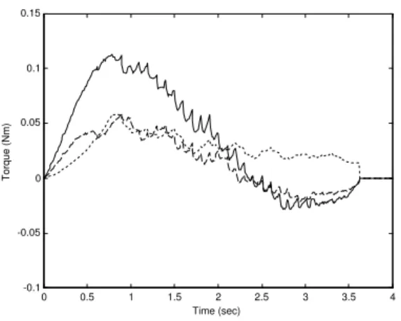
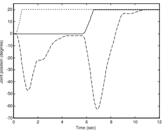
The experimental results: joint positions, joint velocities and applied torques, for the configuration PAP, with
T = [1.0 4.0 0.7 3.0] sec., are shown in Figures 13, 14, and 15, respectively.
0 2 4 6 8 10 12 -70
-60 -50 -40 -30 -20 -10 0 10 20
Time (sec)
Joint position (degrres)
Figure 13: Joint positions, configuration PAP.
0 2 4 6 8 10 12 -80
-60 -40 -20 0 20 40 60
Time (sec)
Joint velocity (degrres/sec)
Figure 14: Joint velocities, configuration PAP.
0 2 4 6 8 10 12 -0.4
-0.3 -0.2 -0.1 0 0.1 0.2 0.3 0.4 0.5
Time (sec)
Torque (Nm)
Figure 15: Applied torques, configuration PAP.
6
CONCLUSION
manipu-lators. Since theMcc(.) andCcc(., .) matrices from (16)
are formed by components ofM(.) andC(., .) matrices, respectively, keeping their proprieties, the solution for the underactuated problem is equivalent to the fully ac-tuated case. The experimental results presented in this paper validate the proposedH∞controller for fully actu-ated and underactuactu-ated manipulators. The application of linear parameter varying (LPV) techniques (Huang and Jadbabaie, 1998) to solve the robotic H∞ control problem is of author’s interest for further works. The LPV methodology is used to solve nonlinear matrix in-equalities (NLMI) generated by convex characterization of the nonlinearH∞control (Lu and Doyle, 1995).
APPENDIX A
The matricesM(q),C(q,q˙), andG(q) for a 3-link planar manipulator with revolute joints, are given by
M(1,1) =m1lc21+m2 l12+lc22+ 2l1lc2cos2+
m3 l21+l22+lc23+ 2l1l2cos2+2l1lc3cos23+2l2lc3cos3+
I1+I2+I3
M(1,2) =M(2,1) =m2 lc22+l1lc2cos2+
m3 l22+lc32+l1l2cos2+l1lc3cos23+2l2lc3cos3+I2+I3
M(1,3) =M(3,1) =m3 lc23+l1lc3cos23+l2lc3cos3+I3
M(2,2) =m2lc22+m3 l22+lc23+ 2l2lc3cos3+I2+I3
M(2,3) =M(3,2) =m3 lc23+l2lc3cos3+I3
M(3,3) =m3lc23+I3
C(1,1) =−(m2l1lc2sin2+m3l1l2sin2+m3l1lc3sin23) ˙q2−
(m3l1lc3sin23+m3l2lc3sin3) ˙q3
C(1,2) =−(m2l1lc2sin2+m3l1l2sin2+m3l1lc3sin23)×
( ˙q1+ ˙q2)−(m3l1lc3sin23+m3l2lc3sin3) ˙q3
C(1,3) =−(m3l1lc3sin23+m3l2lc3sin3) ( ˙q1+ ˙q2+ ˙q3)
C(2,1) = (m2l1lc2sin2+m3l1l2sin2+m3l1lc3sin23) ˙q1−
m3l2lc3sin3q˙3
C(2,2) =−m3l2lc3sin3q˙3
C(2,3) =−m3l2lc3sin3q˙3( ˙q1+ ˙q2+ ˙q3)
C(3,1) = (m3l1lc3sin23+m3l2lc3sin3) ˙q1+m3l2lc3sin3q˙3
C(3,2) =m3l2lc3sin3q˙3( ˙q1+ ˙q2)
C(3,3) = 0 and
G(1) =m1glc1cos1+m2g(l1cos1+lc2cos12) +
m3g(l1cos1+l2cos12+lc3cos123)
G(2) =m2glc2cos12+m3g(l2cos12+lc3cos123)
G(3) =m3glc3cos123
where mi, li, lci, and Ii are the mass, length, center
of mass and inertia of the i-th link and sini =sin(qi),
sinij =sin(qi+qj),cosi= cos(qi),cosij =cos(qi+qj),
andcosijk =cos(qi+qj+qk).
REFERENCES
Arai, H. (1997). Feedback control of a 3-DOF planar un-deractuated manipulator. Proceedings of the 1997 IEEE International Conference on Robotics and
Automation, Albuquerque, New Mexico, USA, pp.
703-709.
Arai, H. and S. Tachi (1991). Position control of a ma-nipulator with passive joints using dynamic cou-pling.IEEE Transactions on Robotics and Automa-tion, Vol. 7, no. 4, pp. 528-534.
Ball, J. A., J. W. Helton and M. L. Walker (1991).H∞ control for nonlinear systems with output feedback.
IEEE Transactions on Automatic Control, Vol. 38,
no. 4, pp. 546-559, 1991.
Basar, T. and G. J. Olsder (1982).Dynamic
Noncoop-erative Game Theory. Academic Press, New York,
USA.
Basar, T. and P. Berhard (1990).H∞-Optimal Control
and Related Minimax Problems. Birkh¨auser, Berlin,
Germany.
Bergerman, M. (1996). Dynamics and control of un-deractuated manipulators. Ph.D. Thesis, Carnegie Mellon University, Pittsburgh, PA, USA.
Craig, J. J. (1989). Introduction to Robots: Mechanics
and Control. Addison-Wesley, Reading, MA.
Chen, B. S., T. S. Lee and J. H. Feng (1994). A non-linearH∞ control design in robotic systems under parameter perturbation and external disturbance.
International Journal of Control, Vol. 59, no. 2, pp.
439-461.
Chen, B. S. and Y. C. Chang (1997). Nonlinear mixedH2/H∞control for robust tracking design of robotic systems. International Journal of Control, Vol. 67, no. 6, pp. 837-857.
Huang, Y. and A. Jadbabaie (1998). NonlinearH∞ con-trol: an enhanced quasi-LPV approach. Workshop
in nonlinear H∞ control by J. C. Doyle, Caltech,
IEEE Conference on Decision and Control,Tampa,
Florida, USA.
Isidori, A. and A. Astolfi (1992). Disturbance attenu-ation and H∞-control via measurement feedback in nonlinear systems. IEEE Transactions on
Auto-matic Control, Vol. 37, no. 9, pp. 1283-1293.
Johansson, R. (1990). Quadratic optimization of mo-tion coordinamo-tion and control. IEEE Transactions
on Automatic Control, Vol. 35, no. 11, pp.
1197-1208.
Lu, W. M. (1996). H∞ control of nonlinear time-varying systems with finite-time horizon.
Interna-tional Journal of Control, Vol. 64, no. 2, pp.
Lu, W. M. and J. C. Doyle (1991). H∞ control of nonlinear systems via output feedback: controller parametrization.IEEE Transactions on Automatic
Control, Vol. 39, no. 12, pp. 2517 - 2521.
Lu, W. M. and J. C. Doyle (1995).H∞control of non-linear systems: a convex characterization. IEEE
Transactions on Automatic Control, Vol. 40, no. 9,
pp. 1668 – 1675.
Postlethwaite, I. and A. Bartoszewicz (1998). Applica-tion of non-linearH∞control to the Tetrabot robot manipulator. Proceedings of the Institution of Me-chanical Engineers-Part I - Journal of Systems and
Control Engineering, Vol. 212, no. 16, pp 459-465.
van der Schaft, A. J. (1991). On a state space approach to nonlinearH∞control.Systems and Control
Let-ters, Vol. 16, pp. 1-8.