REM WORKING PAPER SERIES
The Policy Mix in the US and EMU: Evidence from a SVAR Analysis
António Afonso and Luís Gonçalves
REM Working Paper 028-2018
February 2018
REM – Research in Economics and Mathematics
Rua Miguel Lúpi 20,1249-078 Lisboa, Portugal
ISSN 2184-108X
Any opinions expressed are those of the authors and not those of REM. Short, up to two paragraphs can be cited provided that full credit is given to the authors.
1
The Policy Mix in the US and EMU: Evidence from a
SVAR Analysis
*
António Afonso
$, Luis Gonçalves
#February 2018
Abstract
We use a SVAR approach to the effects of fiscal and monetary policies, as well as their interactions (policy mix) for the US and the Euro Area (EMU). Overall, our results show that these two cases are different from each other. First, while in the case of the US there is evidence of Keynesian monetary policy, the same is not true in the case of the EMU. Second, considering the effects of the global economic and financial crisis, there is evidence of non-Keynesian fiscal policy in the case of the EMU (expansionary fiscal consolidation), while it does not hold in the case of the US. Third, there is evidence supporting the traditional inverse relationship between monetary policy interest rates and inflation in the case of the US, whereas in the case of the EMU there is a price puzzle (frequent in SVAR studies). Fourth, the baseline model seems to be robust in the case of the US, when considering the effects of the economic and financial crisis 2007-2009, while the opposite holds in the case of the EMU. However, in both cases, the policies seem to act as complements. Another similarity appears when analysing the relationship between public spending and taxation, where there is evidence supporting a fiscal retrenchment.
JEL: E52, E61, E62, E63, H50, H60
Keywords: Fiscal Policy, Monetary Policy, Crisis, Unconventional Monetary Policy, US, EMU
* The opinions expressed herein are those of the authors and do not necessarily reflect those of their employers. $ ISEG-UL – Universidade de Lisboa; REM – Research in Economics and Mathematics, UECE – Research Unit on Complexity and Economics. R. Miguel Lupi 20, 1249-078 Lisbon, Portugal. UECE is supported by FCT (Fundação para a Ciência e a Tecnologia, Portugal), email: [email protected].
2 1. Introduction
Since the 1990s, there is a consensus in favour of the separation of powers of monetary and fiscal policies to achieve the main objective of economic policy, i.e., a sustained non-inflationary growth or at least both policies should be used to stabilise the economy (Sprinkel, 1963).
The topic of fiscal and monetary interactions has gained renewed importance in the last years because of the effects of the 2007-2009 economic and financial crisis: regarding monetary policy, central banks lowered aggressively their policy interest rates, although their ability to do so became constrained at the ELB (Effective Lower Bound); regarding fiscal policy, governments launched expansionary packages to recover the sharp decline in output verified during this period, as well as the large increase in unemployment. The result was the following: the central banks could not lower further their policy rates and the governments saw their levels of deficits and debts rise to historic levels, which led to a new discussion related to unconventional monetary policies and fiscal consolidation.
In this paper, we develop an empirical study using the SVAR approach (Sims, 1980) to analyse the policy mix in the Euro Area (EMU) and in the US. One limitation is inherent to the data for the Euro Area, as it masks important heterogeneity across countries, namely relative to those where the crisis had a significantly higher impact. Nevertheless, the SVAR is a widely used methodology to analyse the transmission of macroeconomic policies to macroeconomic variables in several studies, as it provides useful tools such as impulse response functions to analyse the response of each variable in the model to another along time. Then, our main objective in this work is to perform an analysis of the effects of fiscal policy and monetary policy, as well as their interactions, and we also provide a short analysis of the causality between public spending and taxation through applying a SVAR model.
Our results show that in the case of the US there is evidence of Keynesian monetary policy, the same is not true in the case of the EMU. Moreover, there is evidence of the traditional inverse relationship between monetary policy interest rates and inflation in the case of the US, whereas in the case of the EMU there is a price puzzle (frequent in SVAR studies).
In section 2, we present the relevant literature review for our topic. In section 3, we analyse the data and underline important patterns of it during the critical periods (2007-09 and 2010-12), to anticipate important relations for future policy, the econometric framework used in our study, as well as the empirical analysis of our results. In section 4, we perform a robustness check by assessing how the model works with alternative variables. Finally, section 5 concludes.
3 2. Literature Review
Sargent and Wallace (1981) were the pioneers in this study of the policy mix. Indeed, they conclude that if the fiscal authority sets its budgets independently from the monetary authority, then the latter might be forced to tolerate a higher inflation rate than it would prefer to generate sufficient revenue from seigniorage to satisfy the government budget constraint:
𝑏 = 𝑏 + 𝑔 − 𝜌 − − 𝑧 (1) where 𝑏 is the debt ratio, 𝑟 is the real interest rate, 𝑦 is the real GDP growth, 𝑔 is the primary government spending (%of GDP), 𝜌 is the government revenue (% of GDP), 𝑀 is the nominal monetary base, 𝑃 is the price level, 𝑌 is the real GDP, and 𝑧 represents the possibility of the government selling assets, i.e., privatizations (% of GDP).
Rossi and Zubairy (2011) resume that separately considering either monetary policy or fiscal policy is a literature lack, which we think it was only committed in the past. Indeed, their findings are provided in form of new stylised facts: (i) fiscal and monetary policy shocks have different effects on macroeconomic fluctuations, depending on their frequencies and (ii) failing to consider fiscal and monetary variables simultaneously leads researchers to incorrectly attribute economic fluctuations to the wrong source.
Apart from the ‘pioneers’ mentioned above, there are other theories related to the subject of policy mix (see Walsh, 2010). The most remarkable theories are: (i) the Fiscal Theory of the Price Level (FTPL), (ii) strategic interactions between fiscal and monetary policies, and (iii) empirical studies.
The FTPL was initially developed by Leeper (1991), Sims (1994) and Woodford (1994, 1995). The idea is that the price level is determined via the intertemporal government budget constraint in such a way that the price level adjusts to ensure that the current real value of the outstanding government debt equals the present real value of future government primary balances. Given that, this is a less orthodox view relative to Sargent and Wallace (1981) because in the latter the price level is still a monetary result. The major difference between these two relies on the possibility of non-Ricardian regimes, which would be a favourable aspect to validate the FTPL. Several discussions and empirical assessments were conducted (McCallum, 2001; Buiter, 2002; Canzoneri, Cumby and Diba 1996, 2001; Cochrane, 2001; Afonso, 2008). Although each case has its own characteristics, overall the evidence points in favour of Ricardian regimes, i.e., invalidation of the FTPL.
The theory about strategic interactions between fiscal and monetary policies is centred on game theory. Dixit and Lambertini (2003) show that it is reached a type of non-cooperative
4
equilibrium which results in values for GDP and inflation very different from the ones desired due to divergent objectives of the two authorities. Similar conclusions were found by Buti et al. (2001).
Empirical studies focus on the relation of complementarity/substitutability between the two policies. Mélitz (2000) show that coordinated macroeconomic policy exists, i.e., the two policies tend to move in opposite directions, thus being strategic substituents, as well as Wyplosz (1999) and von Hagen et al. (2001). Sometimes, and as we will do in this paper, the authors settle a comparison between the US and the Euro Area, two of the major economies worldwide. For example, van Aarle et al. (2003) shows that in a SVAR model to analyse the transmission of monetary and fiscal policy in the EMU, the Euro-Area estimated adjustments to the various structural shocks are found comparable to the case of US. Peersman and Smets (2001) also show the similarity between the US and the Euro Area, although the data used took the range from 1980 to 1998, i.e., this period does not consider the period in which neither the Stability and Growth Pact nor the single monetary policy had influence. Apart from that, this work is also important in such a way that it analyses the impact of monetary policy on other macroeconomic variables, such as labour market variables, asset prices, investment, and private consumption.
Even though it is not the central idea of this paper, another issue we can analyse is the interdependency between government spending and revenues. It is particularly important due to the recent years of unsustainable public finances worldwide, although it cannot be only attributable to this relationship between government spending and revenues. There are two views on this subject: (i) “tax and spend” and (ii) “spend and tax”. Blanchard and Perotti (2002) use a fiscal SVAR model to analyse both types of causality between government spending and taxation, and one can find the positive relationship between government spending and taxes, although the latter increase less than the former which may indicate unsustainable public finances.
There is a question about the significance of the policy effect on the business cycle, even though there is some consensus on transmission mechanisms. Korenok and Radchenko (2004) resume that monetary policy shocks do not play an important role in cyclical fluctuations, where these shocks are known as monetary policy interest rate shocks. Additionally, during the 2007-09 crisis, the sovereigns relied heavily on fiscal policy due to the limited room for manoeuvre for monetary policy in the presence of the zero-lower bound (ZLB) for nominal interest rates (Blanchard et al., 2010).
5
As we mentioned above, the topic of the policy mix gained renewed importance in the recent years because of the crisis, namely when the governments have seen themselves with limited room for manoeuvre because the substantial increase on the deficit and debt ratios caused by the fiscal stimuli launched during the ZLB period. Therefore, both fiscal and monetary policies were limited to correct the economic fluctuation caused by the crisis. Indeed, Alcidi and Thirion (2016) present an overview of the policy mix before and after the crisis in the EMU, US and UK. During the period 2000-15, the policy mix appears to be to some extent different in the EMU relative to the US. In terms of monetary policy, the inverse relationship between interest rates and inflation is weaker over the period after the crisis and less reliable since the interest rate is not a good proxy for monetary policy. In terms of fiscal policy, the EMU reacted in a more conservative way to the crisis due to three factors: fiscal rules, sovereign crisis (which resulted in a loss of access to the credit market because of the imposed market discipline) and fiscal cost of supporting financial institutions. They conclude with future challenges for policymakers, namely the need to consider financial stability in the definition of the policy mix. Blanchard et al. (2013) provided new ways of acting for policymakers. In terms of monetary policy, the central banks should start targeting economic activity and financial stability, as well as to perform forward guidance and to avoid providing liquidity to nonbanks, given that the limited information possessed by central banks could lead to a liquidity crisis. In terms of fiscal policy, there should be a more comprehensive approach to measure public debt and lower thresholds for the debt ratio. Another important aspect is the risk of fiscal dominance caused by the need for difficult fiscal adjustment because the government would put pressure on the central banks to help limit borrowing costs, which in turn would jeopardise the central banks’ independence, as well as raise an issue on the risks of fiscal activism for inflation volatility (see Afonso and Jalles, 2017). In the end, they also analyse macroprudential instruments as guides for future policy, which we leave for future research due to the limited space in a unique paper. In terms of unconventional monetary policies (UMP), Kozicki et al. (2011) provide an important survey of the types of central bank asset purchases, evidence on these purchases, difficulties to decide when exiting from UMP and potential costs of it. Overall, the measures of quantitative easing (QE) were positive for the macroeconomic environment (see for example Baumeister and Benati, 2010; Chung et al., 2011; Afonso and Kazemi, 2018). However, UMP are only effective under specific circumstances, such as when targeted to address a specific market failure and enhanced by clear communication. Moreover, there is a trade-off in exiting from UMP since an overly aggressive exit, namely in the face of fiscal retrenchment, would eventually push back economies into recession, while an excessively delayed exit would lead
6
to excessive liquidity in the economy, as well as bring inflationary pressures. Finally, UMP also bring potential costs, such as financial market distortions, potential loss of central banks’ independence and credibility, and not less important a delay of necessary macroeconomic adjustments.
3. Methodology
3.1. Data and Analysis
We use quarterly data from 1990:1 to 2016:4 for the US and from 1995:1 to 2016:4 for the EMU (tables I.A and I.B specify the data sources, definitions and transformations for the US and for the EMU, respectively).
[Table I.A] [Table I.B]
Although we argue that each case has its own properties and there is an important difference between these economies (the US is a market-based economy and the EMU is a bank-based economy), we conduct this study to compare the policy mix between the two economies and to see how the policy mix has changed due to the financial crisis and sovereign crisis (EMU), if any.
The variables of our interest for this paper were the output gap/output growth, the capb (cyclically adjusted primary balance), the debt ratio, a proxy for the policy interest rate (EONIA for the EMU and the Federal Funds Rate for the US), inflation and assets held by the central bank. We also collected data on government spending and tax revenues, to analyse how these two parts of the budget balance react and to check the causality between them, and on a financial stress indicator (CISS, Composite Indicator of Systemic Stress, for the EMU and the FSI, Financial Stress Index, for the US).
In Figure 1, we present the relevant figures for the US. Relative to the annual real GDP growth, there is a sharp decrease from 2007: Q3 to 2009: Q2, where the latter represents the turning point of the subprime crisis (the growth rate was approximately -4.1%). The recovery afterwards lasted until 2010: Q3, when the annual growth rate attained 3%. Then, there is a stabilised growth rate until the end of 2016, where it was always positive. In terms of annual inflation, it rarely was in the objective “close to 2%”. The more relevant volatility is related to the subprime crisis, where the annual inflation rate ranged from 5.1% in 2008: Q3 to -1.6% in 2009: Q3. Relative to monetary policy, analysing the graph which combines the FFR (Federal Funds Rate) and the output gap, we can see the aggressive cut in the FFR from 5.3% in 2007:
7
Q3 to 0.1% in 2009: Q4. In fact, both the output gap and the annual real GDP growth rate did not recover as expected by the interest rate mechanism of traditional monetary policy.
[Figure 1]
Furthermore, the output gap started to recover in 2009: Q3, as well as the annual real GDP and so other factors may be related to both recoveries since the FFR persisted close to its ZLB. In terms of fiscal policy, there is an aggressive cut in the capb (expansionary fiscal policy) from 2007: Q1 to 2010: Q3 that did not have the expected result in both output gap and real GDP growth, followed by a strong fiscal consolidation afterwards until the end of the sample. By looking at the behaviour of the capb during the whole sample one could say that the Keynesian effects of fiscal policy were outweighed by non-Keynesian ones. However, there is still a discussion about the measures of discretionary fiscal policy through the capb, but this is a discussion outside from our plan in this paper. Analysing specifically some parts of the budget balance, such as the real values of public spending and taxes, we can see that the latter is always below the former and this relationship aggravates during the 2007-09 crisis (it is still persistent afterwards) which may also indicate non-discretionary adjustments of these variables, i.e., during that crisis there were simultaneous increases in public spending and decreases in taxes due to higher unemployment (higher unemployment subsidies and lower tax revenues on personal income). Not surprisingly, the debt-to-GDP ratio substantially increases from 64% in 2008: Q2 to 102% in 2013: Q1 which reflects in part the behaviour of subsequent deficits. Relative to the policy mix, one could argue that overall fiscal and monetary policies act as complements, i.e., they tend to move in the same direction. During the 2007-2010 period, we can observe both expansionary fiscal and monetary policies which have not resulted in economic growth. Finally, we present the factors we consider to be determinant for the recovery of real GDP annual growth rate and, therefore inflation: unconventional monetary policy (e.g. quantitative easing, QE) and a sustained decrease of above-average financial market stress (measured by the FSI). The graph of total assets of all Federal Reserve banks show the successive QE measures in the US: 2008: Q3-2010: Q1 (QE1), 2010: Q4-2011: Q3 (QE2) and 2012: Q3-2014: Q4 (QE3). In its turn, the FSI attained the maximum level of 4.25 in 2008: Q4 and then it decreased to negative values, where it stays until today, representing below-average financial market stress.
In Figure 2, we present the relative figures for the EMU. Relative to annual real GDP growth, there was a sharp decrease from 3.8% in 2007: Q2 to -4.3% in 2009: Q2. Then, there was a significant recovery until 2010: Q4 when the growth rate attained 1.7%. However, there were some countries that began a new recession in this period, namely Portugal, Ireland, Italy,
8
Greece and Spain which contributed to a significant decrease of the annual real GDP growth rate to -2.3% in 2012: Q3. Aftermath, there was a recovery and this growth rate started to be positive in 2013: Q4, and it stayed to be until nowadays. In terms of inflation, we can see that its volatility started with the 2007-09 crisis, as before it was above but “close to 2%”. Indeed, there are two periods in which the annual inflation rate decreased a lot: (i) during the “subprime crisis” it decreased from 3.8% in 2008: Q3 to -0.4% in 2009: Q3 and (ii) during the “sovereign crisis” it decreased from 2.9% in 2011: Q4 to -0.3% in 2015: Q1.
[Figure 2]
Relative to monetary policy, one could say that the traditional monetary transmission mechanism started to change in the 2000s, as the EONIA and the output gap started to move in the same direction, while it should move in the opposite. Again, we can see the ECB cutting one of its policy rates from 4.3% in 2008: Q3 to 0.4% in 2009: Q4 to stimulate the economy, but ending in the ZLB without having a significant effect on both the output gap and the real GDP growth rate. Interestingly, from 2015: Q1 to the end of the sample period the EONIA is negative, which reflected a new case study for the Euro Area: the possibility to overcome the ZLB with negative interest rates. Relative to fiscal policy, we can see also the behaviour related before: there was a significant expansionary fiscal policy during the 2007-09 period without influencing both the output gap and the real GDP growth rate. Again, as in the US case, one could say that the Keynesian effects were not valid during this sample because the output gap seems to move in the same direction of the capb, but again the discussion of the measures of discretionary fiscal policy is outside from the plan of this paper. As in the US, the level of real taxes was always below the level of real public spending and this relationship also aggravates from 2008 afterwards. However, it was not as grave as in the US which can be explained by the rules presented in the Stability and Growth Pact effective in the EMU. Again, not surprisingly the debt ratio started to increase from 65.84% in 2008: Q1 to 93.07% in 2014: Q2. The more severe aggravation in the US may be in part explained by a higher fiscal stimulus launched in that area than in the EMU, as well as the fiscal retrenchment lived in the EMU during and after the sovereign crisis, usually dated from 2010 to nowadays. For curiosity, it is interesting that the debt-to-GDP ratio computed for the Euro Area was never below or at the threshold of 60% present in the Stability Growth Pact and recently shown as the “prudent debt level” (Andrés et al., 2017). Relative to the policy mix, one could argue that fiscal and monetary policy act as complements, as observed in the case of the US, except for the 1995-1999 which could reflect a change in the paradigm of the policy mix with the creation of the single monetary union. The same pattern observed in the US is observed in this case, as we see in 2009 both monetary and
9
fiscal policies being without room for manoeuvre. Although there is no such reference value for the CISS as in the case of the FSI for the US, it shows substantial increases during the 2007-2009 period, as well as during the 2010-2011/12 period reflecting both the effects of the global economic and financial crisis and the (Greek) sovereign crisis with its contagion across the EMU countries. Finally, the ECB assets graph represents a proxy for the unconventional monetary policies carried out in the EMU. The most relevant changes were from 2011: Q2 to 2012: Q3 and from 2015: Q1 to 2016: Q4, where the latter corresponds to the introduction of QE in the EMU which occurred much later than in the US (see Driffill (2015) for a discussion).
3.2. Econometric Framework
Macroeconomic phenomena are characterised by feedback and reciprocal causality, and so we analyse the effects of fiscal policy and monetary policy, as well as their interaction, and provide a short analysis of the causality between public spending and taxation through applying a structural VAR (SVAR) model.
Introduced by Sims (1980), VAR models have been widely used in analysing monetary and fiscal shocks, both integrated and separated, and their effect on the real economy. In its turn, the SVAR approach was pioneered by Blanchard and Quah (1989), concentrating on long-run identifying restrictions to identify demand and supply shocks hitting the economy. Monticelli and Tristani (1999) use a SVAR approach to analyse the transmission mechanism of aggregate demand shocks, aggregate supply shocks and monetary policy shocks in the aggregate EMU. SVAR models require a minimum set of restrictions and offer useful instruments, such as impulse response functions (see van Aarle et al. (2003) for an overview of advantages and limitations of this methodology). Other useful instruments, such as the Granger causality tests and forecast error variance decomposition (FEVD) will not be considered throughout this paper. In this paper, we include both monetary and fiscal variables, as Favero (2002) has shown that a separate estimation of monetary and fiscal policies effects would lead to biased estimators, hence reinforcing the importance to study the policy mix, instead of separated macroeconomic policies effect.
Now, we describe a benchmark SVAR model to analyse the topics described above: 𝐴𝑌 = 𝐺(𝐿)𝑌 + 𝐶(𝐿)𝑋 + 𝐵𝑣 (2) Where A represents a (𝑛𝑥𝑛) matrix of long-run relations, 𝑌 represents a (𝑛𝑥1) vector of endogenous macroeconomic variables, 𝐺(𝐿) and 𝐶(𝐿) represent lag operators, 𝐵 represents a diagonal matrix, 𝑋 represents a (𝑛𝑥1) vector of exogenous variables and 𝑣 represents the (𝑛𝑥1) structural innovations vector.
10
Equation (2) presents the structural model of the economy, which cannot be empirically observed. On the other hand, by solving that equation to 𝑌 we get the reduced-form model, whose shocks 𝜇 = 𝐴 𝐵𝑣 can be observed. Here, the identification problem emerges, which we will turn later.
We use two different sets of endogenous variables in this benchmark model. The first one is 𝑌 = (𝑦 , 𝑐𝑎𝑝𝑏 , 𝑖 , 𝜋 ) and the second is 𝑌 = (𝑦 , 𝑡 , 𝑔 , 𝑖 , 𝜋 )′, where 𝑦 represents the real GDP, 𝑐𝑎𝑝𝑏 is the cyclically adjusted primary balance, 𝑖 is the proxy for the monetary policy rate (the Fed funds rate for the US and the EONIA for the EMU), 𝑡 represents the real tax revenues, 𝑔 represents the real total government spending and 𝜋 represents the inflation rate. In the case of 𝑋 , in the benchmark models it is defined as 𝑋 = (𝑎𝑠𝑠𝑒𝑡𝑠 ) and in the alternative model it is defined as 𝑋 = (𝑎𝑠𝑠𝑒𝑡𝑠 , 𝑐𝑟𝑖𝑠𝑖𝑠 ), where 𝑎𝑠𝑠𝑒𝑡𝑠 represents the assets held by each central bank and 𝑐𝑟𝑖𝑠𝑖𝑠 represents a dummy variable to isolate the effect of the crisis, which assumes the value of 1 from 2008:Q4 until the end of the sample. In table 2 we present the specifications formally.
[Table II]
All in all, we estimate 4 models for the US and the EMU. The reasonable comparisons are between model 1 and model 3, as well as between model 2 and model 4, in terms of analysing the effect of introducing the dummy variable in the model. The difference between models 1 and 2, as well as between 3 and 4, is that in the odd we consider the capb and in the even we consider both the revenue and spending parts of the budget balance. Naturally, it is also reasonable to settle a comparison between the two cases of US and EMU.
3.3. Empirical Analysis
In this section, we analyse the results of our benchmark models. For simplicity, we will analyse separately the economies and then we make a comparison between the two.
3.3.1. The case of US
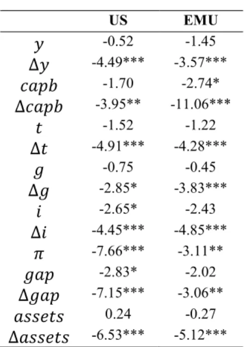
Before running the model, it is adequate to check whether all series included in the model are stationary. Table 3 provides the results of the augmented Dickey-Fuller (ADF) tests for each variable. Indeed, the tests indicate that the series are non-stationary (except inflation) and these have different orders of integration (GDP, policy rate, capb and assets are I(1), while public spending is I(2)). For this reason, we decide to implement the following vectors of endogenous and exogenous variables respectively 𝑌 = (∆𝑦 , ∆𝑐𝑎𝑝𝑏 , ∆𝑖 , 𝜋 ) and 𝑋 = (∆𝑎𝑠𝑠𝑒𝑡𝑠 ), where
11
∆𝑦 is the real GDP growth, ∆𝑐𝑎𝑝𝑏 is the change in the capb, ∆𝑖 is the change in the Federal funds rate, 𝜋 is the inflation rate and ∆𝑎𝑠𝑠𝑒𝑡𝑠 is the change in the assets held by all the Federal Reserve banks.
[Table III]
Therefore, this model is driven by four structural shocks: an aggregate supply shock, 𝑣 , a fiscal shock, 𝑣 , a monetary shock, 𝑣 , and an aggregate demand shock, 𝑣 . In the second specification, the model is driven by five structural shocks: an aggregate supply shock, 𝑣 , a real government taxes shock, 𝑣 , a real government spending shock, 𝑣 , a monetary shock, 𝑣 , and an aggregate demand shock, 𝑣 .
Relative to the identification problem, it is in practice solved by imposing identifying restrictions. As we are simulating a structural VAR and economic theory provides more guidance about long-run relationships rather than short-run dynamics, we impose long-run identification restrictions as in Blanchard and Quah (1989). Moreover, we have macroeconomic theories to impose this kind of restrictions, such as the AS-AD model. In practice, we need to identify 6 restrictions for the 1st specification and 10 restrictions for the 2nd one (we will follow van Aarle et al. (2003) for the 2nd specification of the benchmark model).
Thus, in the 1st specification we apply the following restrictions: (i) fiscal shocks do not have a permanent effect on real output, because of the long-run neutrality of fiscal policy supported by Ricardian equivalence; (ii) monetary shocks do not have a permanent effect on real output, because of the long-run neutrality of money (McCandless and Weber, 1995; Christiano et al., 1999).; (iii) aggregate demand shocks do not have a permanent effect on real output (Blanchard and Quah, 1989); (iv) monetary shocks do not have a permanent effect on fiscal policy, because of the possibility of the fiscal authority setting its budgets independently from the monetary authority (Sargent and Wallace, 1981); (v) aggregate demand shocks do not have a permanent effect on fiscal policy, because of the smallness and temporariness of fiscal policy shocks (Friedman, 1972), the fiscal authority will not react to aggregate demand shocks in the long run; (vi) aggregate demand shocks do not have a permanent effect on monetary policy because of the non-clarity of the effects of the former on the latter as Barro (1987) highlighted the inconsistency between theory and data, and namely the empirical evidence to the US supports this idea (Murphy and Walsh, 2015).
Then, in the 2nd specification (van Aarle et al., 2003): (i) real government taxes shocks do not have a permanent effect on real output; (ii) real government spending shocks do not have a permanent effect on real output; (iii) real government spending shocks do not have a permanent
12
effect on real government taxes; (iv) monetary shocks do not have a permanent effect on real output; (v) monetary shocks do not have a permanent effect on real government taxes; (vi) monetary shocks do not have a permanent effect on real government spending; (vii) aggregate demand shocks do not have a permanent effect on real output; (viii) aggregate demand shocks do not have a permanent effect on real government taxes; (ix) aggregate demand shocks do not have a permanent effect on real government spending; (x) aggregate demand shocks do not have a permanent effect on the monetary policy interest rate.
We have run a model up to 2 lags in both specifications. From the reduced-form model, we could conclude that the model satisfies the hypotheses of homoscedasticity and absence of autocorrelation, and the model is also stable (the inverse roots of AR characteristic polynomial lie inside the unit circle). Relative to normality, this hypothesis was relatively rejected, but this is an expected result because the number of observations is not high enough to satisfy this property, and so the test has low power.
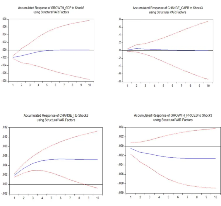
Then, impulse response functions can be calculated from the estimated SVAR models (structural decomposition of innovations), which show the effects of the shocks we are interested in analysing. The accumulated effects on growth rates reflect the effects on the level of the endogenous variables, in each period. Quantitatively, a response of 0.01 corresponds to a 1% change in the variable of interest (𝑦, 𝑡, 𝑔, 𝜋), while the same 0.01 corresponds to a 1 p.p. change in the others (𝑖, 𝑐𝑎𝑝𝑏). Figures 3 and 4 show the impulse response functions to fiscal and monetary shocks in model 1, for the US. At the same time, figures 5 and 6 show the impulse response functions to taxes and monetary shocks in model 2, for the US12. For reasons of statistical significance, we neglected the analysis of spending shocks in the two figures of both models 2 and 4 in both cases of the US and EMU. Nevertheless, it is available on request. Model 1: (i) supply shocks (results on request) result in an increase in real output; in terms of policy, both the fiscal and monetary authorities conduct restrictive fiscal and monetary policies to cool the economic growth, where latter is statistically significant until the 7th quarter; (ii) demand shocks (results on request) result in an increase in inflation; in terms of policy, both fiscal and monetary policies became restrictive to cool the economic growth and sustain inflationary pressures, although the government reaction is statistically significant until 3 quarters from now whereas the Fed reaction is statistically significant during 1 quarter; (iii)
1 The IRFs of AS and AD shocks, as well as the IRFs of models 3 and 4 are available on request. In the case of the EMU, we will perform in the same way.
2 Below the figures, we identify the shocks (EViews does not do it when using accumulated IRFs). We did the same for the EMU figures.
13
fiscal policy shocks show Keynesian effects, i.e., a restrictive fiscal policy results in a lower real output (statistically significant during 3 quarters);
[Figure 3]
(iv) monetary policy shocks show the traditional interest rate mechanism, i.e., an increase in the FFR results in a decrease of real output, even though these results are not statistically significant; (v) relative to the fiscal and monetary interactions, the capb hardly reacts to the FFR, while the FFR seems to act as a complement to the capb, i.e., both fiscal and monetary policies seem to move in the same direction, even though the result is not statistically significant; nevertheless, the complementary reaction of these capb and FFR to aggregate supply shocks may lead us to conclude that the policies are working as complements.
[Figure 4]
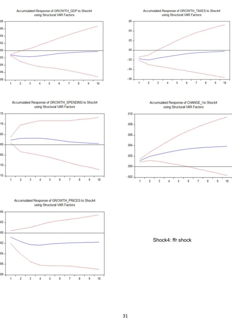
Model 2: (i) supply shocks (results on request) result in an increase on real output and in a decrease on inflation, although the latter is not significant and disappears after 6 quarters; in terms of policy, both fiscal and monetary policies become restrictive (increase on FFR, increase on taxation and decrease on public spending, although the latter is not statistically significant), wherein the case of fiscal policy it is taxation changing more relatively to spending; (ii) demand shocks (results on request) result in an increase on real output and an increase on inflation, although the former is not significant; (iii) fiscal policy shocks show Keynesian effects both on the revenue and spending sides, i.e., an increase on taxation is followed by a decrease on real output (statistically significant during 2 quarters) and an increase on public spending is followed by an increase on real output (not statistically significant);
[Figure 5]
(iv) monetary policy shocks remain unchanged from the perspective of model 1, i.e., an interest rate hike results in a decrease on real output, as well as in a decrease on inflation, although these results are not statistically significant; (v) in terms of fiscal and monetary interactions, the results are more significant in the sense of complementarity, i.e., increases in FFR result in decreases on taxation (substituents) and in increases on public spending (substituents), although the latter is not significant and the former is statistically significant during 3 quarters; increases in taxation result in increases on the FFR (complements) and increases in public spending result in decreases on the FFR (complements), where the former is statistically significant during 7 quarters and the latter is not significant at all; overall, we could say that complementarity between policies dominates substitutability; (vi) analysing the causality between public spending and taxation, there is evidence in favour of the “tax and spend” view because changes
14
in public spending follow changes in taxation3; nevertheless, there is no clear causality between taxation and spending, given that an increase in taxation is followed by a decrease in public spending, which could mean a path towards public finance stability (fiscal retrenchment); furthermore, all these results are not statistically significant.
[Figure 6]
Model 3 (results on request): comparing to the 1st model, the unique remarkable change is in the case of supply shocks, wherein this model the inflation rate increases, instead of decreasing even though the results are not significant; to some extent, there are some quantitative changes, but the fundamentals on how policy reacts and its effects on the main macroeconomic variables remain unchanged, and so the 1st model is robust to the dummy variable introduced to isolate the effects of the crisis.
Model 4 (results on request): comparing to the 2nd model, the unique remarkable change is in the study of causality between public spending and taxation; in this model, it seems that the evidence points for the “spend and tax” view; indeed, and as it is not the main objective of this paper, this change may be due to the limited capability of this SVAR model to analyse such issue; moreover, the result of absence of clear causality remains valid in this last specification, as well as the result of statistically insignificance.
Overall, the models remain robust to the periods of the crisis which may indicate that other variables which were not included as endogenous in this specification motivated the use of unconventional monetary policies in the US. The qualitative results are in line with other studies using this approach and with economic theory, e.g. the AS-AD model in the case of supply and demand shocks.
3.3.2. The case of EMU
To make the models comparable between the US and the EMU, we have run the same models in the same specifications and with the same endogenous4 and exogenous variables. The only difference is that we have run a model up to 4 lags in both specifications5. The main reason for that was the need to satisfy the basic properties of stability, homoscedasticity and absence of autocorrelation. Again, usually the normality hypothesis was relatively rejected, but the sample period, in this case, is even more limited and so the test has low power. At the same
3 Keep in mind that restriction (iii) in the 2nd specification rules out any impact from spending on taxation in the long run.
4 Check table 2A for the ADF stationarity tests.
5 Another difference is that both the capb and the EONIA were used in levels, in model 1. Again, it has been done to satisfy the basic properties of stability, homoscedasticity and absence of autocorrelation.
15
time, we imposed the same set of restrictions for the EMU and the quantitative interpretations done in the case of US remain valid here. Figures 7 and 8 show the impulse response functions to fiscal and monetary shocks in model 1, for the EMU. At the same time, figures 9 and 10 show the impulse response functions to taxes (fiscal) and monetary shocks in model 2, for the EMU. Again, for reasons of statistical significance, we neglected the analysis of spending shocks in the last two figures and this is available on request.
In practice, in this section, we will present the results of each model and settle a comparison between the impulse response functions in the EMU and in the US.
Model 1: (i) supply shocks (results on request) result in an initial decrease in real output ,and in an increase afterwards, and in a decrease in inflation (the former result is not statistically significant); in terms of policy, fiscal policy becomes restrictive while monetary policy becomes expansionary which may suggest the different objectives between the fiscal and monetary authorities, i.e., the monetary authority could be viewed as obsessed with inflation neglecting the output growth and the fiscal authority just caring with output growth, which is a good signal for public finance, neglecting inflation; (ii) demand shocks (results on request) result in an increase in both real output and inflation, where the former is statistically significant during 4 quarters; in terms of policy, both fiscal and monetary policies become restrictive, although the results are not significant at all; (iii) fiscal policy shocks show Keynesian effects, i.e., a restrictive fiscal policy is followed by a decrease in real output; an interesting result is that inflation reacts positively to a shock in fiscal policy, which might indicate a mechanism worth of a further study relating fiscal activity and prices;
[Figure 7]
(iv) monetary policy shocks invalidate the view of the traditional interest rate mechanism, i.e., an interest rate hike is followed by an increase in real output (non-Keynesian monetary policy), and there is a price-puzzle which is common to the SVAR literature, i.e., an interest rate increase is followed by an increase in inflation (see Sims, 1992); two other reasons may justify this price-puzzle which would be either the effectiveness of EONIA to control inflation is reduced or this EONIA would be a bad proxy for monetary policy, possibly because after the ZLB period the interest rate is not anymore a good proxy for monetary policy measures; (v) in terms of fiscal and monetary interactions, the EONIA hardly reacts to the capb, while an increase in the EONIA is followed by an increase on the capb, and so there is evidence of complementarity between fiscal and monetary policies.
16
Model 2: (i) supply shocks (results on request) result in an increase on output and a decrease on inflation; in terms of policy, both policies become expansionary until the 5th quarter (decrease on the interest rate and the increase on public spending is higher than the increase on taxation, where the former is not statistically significant) and then they become both restrictive (the increase on taxation is higher than the increase on public spending, as well as the EONIA starts to increase); (ii) demand shocks (results on request) result in an increase on both real output and inflation; in terms of policy, both become restrictive (increase on both taxation and interest rate, as well as decrease on public spending); (iii) fiscal policy shocks show Keynesian effects in the revenue side on real output, although it is not significant, and non-Keynesian effects in the spending side, until the 4th quarter, and then Keynesian effects; one possible reason could be that non-Keynesian effects were outweighing Keynesian ones initially (see van Aarle and Garretsen, 2003 for a discussion); nevertheless, fiscal policy effects on output growth are not statistically significant in this specification;
[Figure 9]
(iv) monetary policy shocks invalidate the traditional interest rate mechanism and evidence the price puzzle common in the SVAR analysis (statistically significant during 3 quarters in both cases); (v) in terms of fiscal and monetary interactions, there is no clear complementarity or substitutability between the two policies because fiscal policy act as a complement to monetary policy, i.e., interest rate hikes are followed by an increase on taxation and a decrease on public spending, and the interest rate act as a substitute to fiscal policy on the public spending side, i.e., an increase in public spending is followed by an increase on interest rate; relative to taxation, the interest rate act as a substitute until the 4th quarter, although the result is not significant, and then as a complement; however, and taking into account the statistical significance, we could say that the policies act as complements, given that the statistically significant results are the fiscal policy responses to monetary shocks; (vi) analysing the causality between public spending and taxation, there is little evidence on the “spend and tax” view as taxation increases are following increases on public spending, although the result is not statistically significant; furthermore, increases on taxation are followed by decreases on public spending; this is a very interesting result, as the fiscal authority is always seeking for sustainable budget balances (fiscal retrenchment), which in turn may be influenced by the fiscal rules in the Stability and Growth Pact, and because it is statistically significant.
[Figure 10]
Model 3 (results on request): comparing to the 1st model, there are some remarkable changes; (i) relative to supply shocks, the real output shows a different path (and it is now
17
statistically significant) and the fiscal policy reacts differently, i.e., in this model the capb reacts negatively to these shocks, and so the government will set an expansionary fiscal policy to stimulate demand; nevertheless, the fiscal reaction is not statistically significant; monetary policy also becomes expansionary, but it only lasts to the 4th quarter; as in the case of fiscal policy, also this monetary reaction is not statistically significant; (iii) relative to fiscal policy shocks, the real output reacts in an opposite way, i.e., while in model 1 there was evidence of Keynesian effects, in model 3 there is evidence of non-Keynesian effects; additionally, that ‘interesting’ result between fiscal policy and inflation is still positive, but now it is not statistically significant; (iv) relative to monetary shocks, the EONIA lost effectiveness in controlling both output growth and inflation, which stress out that idea of the interest rate not being anymore a good proxy for monetary policy; (v) relative to fiscal and monetary interactions, while in model 1 it was the fiscal policy reacting to monetary policy, in model 3 it is monetary policy reacting to fiscal policy; however, the evidence of complementarity still holds.
Model 4 (results on request): comparing to the 2nd model, there are also some remarkable changes; (i) relative to supply shocks, while in model 2 fiscal policy was expansionary during 5 quarters, in model 4 it is always restrictive; (iii) relative to fiscal policy shocks, while in model 2 there was evidence of Keynesian effects of fiscal adjustments on the revenue side, in model 4 the opposite is verified, although the results are not much significant; furthermore, model 4 shows clear non-Keynesian effects of fiscal adjustments on the spending side, while model 2 only showed it during 4 quarters; however, these results remain statistically insignificant from one specification to the other; (vi) in terms of causality between public spending and taxation, in model 2 increases on public spending were followed by increases in taxation, while in model 4 the opposite holds during 4 quarters (fiscal retrenchment, again), and even afterwards these variables hardly interact, although these results remain statistically insignificant here.
Overall, the qualitative results are in line with other studies using this approach and with economic theory, e.g. the AS-AD model in the case of supply and demand shocks. However, one could conclude that the inclusion of the dummy variable in the case of EMU changes more the results than in the case of US. Particularly in the case of EMU, it faced one more crisis than the US, i.e., the sovereign crisis starting in 2010-11, and so the US economy probably recovered earlier than the EMU, and measures of unconventional monetary policy were also conducted much later than in the case of US. Another important difference is the basis of each economy. In practice, a bank-based economy, as the EMU, may react very differently to the financial
18
crisis than a market-based economy, as the US, but it is a discussion outside our plan which we leave for future research.
The other main differences from the analysis of the impulse response functions may resumed in the following way: (i) relative to supply shocks, monetary policy reacts differently in the US, i.e., while in the EMU it becomes expansionary, in the US it becomes restrictive; the inclusion of the dummy variable affects the reaction of fiscal policy, i.e., while in the EMU it becomes expansionary, in the US it remains restrictive; (ii) relative to demand shocks, both the policy reactions seem to be relatively the same in both areas; (iii) relative to fiscal policy shocks, the Keynesian effects in the US differ relative to the case of EMU essentially in the spending side; the inclusion of the dummy variable clearly changes the effects in the EMU, as while in the case of US the Keynesian effects of fiscal policy remain unchanged, these turn in non-Keynesian effects in the EMU (the crises faced by the EMU may change the fundamentals of direct effects of fiscal policy on real output, while the crisis faced by the US not); (iv) relative to monetary policy shocks, these are clearly different between the two areas, i.e., in the EMU case the traditional interest rate mechanism is always rejected and there is evidence on the price-puzzle result which is common in the SVAR literature whereas in the US case the opposite holds; one possible explanation would be the measure used as a proxy for monetary policy in the EMU, where the ECB has three reference interest rates, and so a unique interest rate as the EONIA could be a bad proxy, whereas the FFR is the unique policy rate used by the Fed; (v) relative to fiscal and monetary interactions, it seems that it is fiscal policy reacting to monetary policy in the EMU case whereas it is monetary policy reacting to fiscal policy in the US case; while in the case of EMU taxation and public spending seem to act as complements to the EONIA, and the EONIA seems to act as substitute to the public spending, in the case of US they seem to act as substitutes to the FFR, and the FFR seems to act as a complement to both taxation and public spending; although there is no clear interaction between the two policies, on average they seem to act as complements in both areas; (vi) relative to the causality between public spending and taxation, although these variables appear to present the same reaction to each other, there is little evidence on the “tax and spend” view in the case of US and on the “spend and tax” view in the case of EMU; the inclusion of the dummy variable changes a bit the comparison, but it is not too significant.
19 4. Robustness Check
Indeed, in the previous section, we performed some robustness check by analysing how the model works including the dummy variable (𝑐𝑟𝑖𝑠𝑖𝑠) and by separating the fiscal policy in spending and revenue sides.
The other most common approaches to performing such a robustness check are dividing the sample period and analysing how the model works in the two different subsamples, changing the order of variables and use other endogenous variables. In our case, the sample periods are not high enough to perform the first approach mentioned above, as well as the second one would not be feasible since there are 𝑛! possible ordering, with 𝑛 being the number of endogenous variables, and if we also did one unique change it would make us to analyse eight different models again in a limited space.
In fact, what we could perform was the third approach mentioned above and we did it. A reasonable alternative endogenous variable we used was the output gap, instead of the real output. However, the results did not change significantly so that we stayed with the original models and making the analysis on different ones would be counterproductive.
5. Conclusion
The discussion about the policy mix has regained importance in the last years due to the 07-09 crisis. The implementation of UMP may affect this policy mix, but such assessment has very limitations (Kozicki et al., 2011).
We have applied a SVAR setup to analyse the policy mix in the US and in the EMU. Bearing in mind the difficulties of using this methodology for future policy and in the specific case of the EMU the mask over heterogeneity across countries, we could find important differences between these two major economies, namely on how both fiscal and monetary policies affect real output and prices. Overall, both policies act as complements in both areas, even though in the EMU the crises may have changed this relationship. In the case of US, the crisis has not changed significantly these results and so other variables may have provoked the non-expected results of both policies (e.g., other than rational expectations).
Comparing to previous studies included in our literature review, the results may have been significantly affected due to the crisis, i.e., the inclusion of more recent data changed the previous results of policies acting as strategic substituents and of similarity between the cases of the US and EMU, given that our evidence suggests that policies are acting as complements and there are some differences between these two cases, namely how both fiscal and monetary policies affect both real output and inflation.
20
Indeed, we do not have a large enough amount of observations to evaluate the effect of UMP in the policy mix, i.e., to forget about the effect of interest rates on inflation since, say, 2010. Additionally, “solving” the problems of such assessment mentioned in Kozicki et al. (2011) may lead us to better assessing how UMP worked, as well as to analyse whether it is temporary or it is going to be part of a new policy toolkit. This is a topic we leave for future research.
References
Afonso, A. (2008). Ricardian fiscal regimes in the European Union. Empirica, 35(3), 313–334. Afonso, A., and Jalles, J.T. (2017). Fiscal Activism and Price Volatility: Evidence from Advanced and Emerging Economies. ISEG Economics Department, WP04/2017/DE/UECE. Afonso, A. and Kazemi, M. (2018). Euro Area Sovereign Yields and the Power of Unconventional Monetary Policy, Finance a úvěr-Czech Journal of Economics and Finance, forthcoming
Andrés, J., Pérez, J., and Rojas, J. A. (2017). Implicit Public Debt Thresholds: An empirical exercise for the case of Spain. Banco de España, WP 1701
Alcidi, C., and Thirion, G. (2016). The interaction between fiscal and monetary policy – before
and after the financial crisis, (649261), 1–22. Retrieved from
http://www.firstrun.eu/files/2016/07/D4.2_Policy_mix_final_ed.pdf
Barro, R. J. (1987). Government spending, interest rates, prices, and budget deficits in the United Kingdom, 1701-1918. Journal of Monetary Economics, 20(2), 221–247.
Baumeister, C., and Benati, L. (2010). Unconventional monetary policy and the great recession - estimating the impact of a compression in the yield spread at the zero-lower bound. International Journal of Central Banking, 9(2), 165–212.
Blanchard, O. J., and Quah, D. (1989). The dynamic effects of aggregate demand and supply disturbances. American Economic Review, 79(4), 655–673.
Blanchard, O., Dell’Ariccia, G. D., and Mauro, P. (2010). Rethinking Macroeconomic Policy: Getting Granular. IMF Staff Position Note, 10(3).
Blanchard, O., Dell’Ariccia, G. D., and Mauro, P. (2013). Rethinking Macro Policy II: Getting Granular. IMF Staff Discussion Note, 1–26.
Blanchard, O., and Perotti, R. (2002). An empirical characterization of the dynamic effects of changes in government spending and taxes on output. Quarterly Journal of Economics, 117(4), 1329–1368.
21
Buiter, W. H. (2002). The fiscal theory of the price level: A critique. Economic Journal, 112(481), 459–480.
Buti, M., Roeger, W., and Veld, J. I. (2001). Stabilizing Output and Inflation: Policy Conflicts and Co-operation under a Stability Pact. Journal of Common Market Studies, 39(5), 801. Canzoneri, M.; and Diba, B. (1996). Fiscal Constraints on Central Bank Independence and Price
Stability, CEPR Discussion Paper 1463.
Canzoneri, M. B., Cumby, R. E., and Diba, B. T. (2001). Is the price level determined by the needs of fiscal solvency? American Economic Review, 91(5), 1221–1238.
Christiano, L. J., Eichenbaum, M., and Evans, C. L. (1999). Monetary policy shocks: What have we learned and to what end? Handbook of Macroeconomics, 1(A), 65–148.
Chung, H., Laforte, J. P., Reifschneider, D., and Williams, J. C. (2012). Have We Underestimated the Likelihood and Severity of Zero Lower Bound Events? Journal of Money, Credit and Banking, 44(SUPPL. 1), 47–82.
Cochrane, J. H. (2001). Long-Term Debt and Optimal Policy in the Fiscal Theory of the Price Level. Econometrica, 69(1), 69–116.
Dixit, A., and Lambertini, L. (2003). Interactions of commitment and discretion in monetary and fiscal policies. American Economic Review, 1522-1542
Driffill, J. (2015). Unconventional Monetary Policy in the Euro Zone. ISEG Economics Department, WP15/2015/DE/UECE
Favero, C. A. (2002). How do European monetary and fiscal authorities behave? CEPR Discussion paper 3426.
Friedman, M. (1972). Comments on the Critics. Journal of Political Economy, 80(5), 906-950. Korenok, O., and Radchenko, S. I. (2004). Monetary Policy Effect on the Business Cycle
Fluctuations: Output vs. Index Measures of the Cycle, 7416(732), 1–45.
Kozicki, S., Santor, E., and Suchanek, L. (2011). Unconventional Monetary Policy: The International Experience with Central. Bank of Canada Review, (Spring), 13–25.
Leeper, E. M. (1991). Equilibria under “active” and “passive” monetary and fiscal policies. Journal of Monetary Economics, 27(1), 129–147.
McCallum, B. T. (2001). Indeterminacy, bubbles, and the fiscal theory of price level determination. Journal of Monetary Economics, 47(1), 19–30.
McCandless, G. T., and Weber, W. E. (1995). Some Monetary Facts. Federal Reserve Bank of Minneapolis Quarterly Review, 19(3), 2–11.
Monticelli, C., and Tristani, O. (1999). What does the single monetary policy do? A SVAR Benchmark for the European Central Bank. ECB WP 2.
22
Melitz, J. (2000), Some Cross-Country Evidence About Fiscal Policy Behaviour and Consequences for EMU, European Economy Reports and Studies 2, 3–21.
Murphy, D., & Walsh, K. (2015). Demand Shocks and Interest Rates.
http://editorialexpress.com/cgi-bin/conference/download.cgi?db_name=MWMSpring2015&paper_id=314
Peersman, G., and Smets, F. (2001). The Monetary Transmission Mechanism in the Euro Area: More Evidence From VAR Analysis. ECB WP 91.
Rossi, B., and Zubairy, S. (2011). What Is the Importance of Monetary and Fiscal Shocks in Explaining U.S. Macroeconomic Fluctuations? Journal of Money, Credit and Banking, 43(6), 1247–1270.
Sargent, T. J., and Wallace, N. (1981). Some Unpleasant Monetarist Arithmetic. Federal Reserve Bank of Minneapolis Quarterly Review 5, 1-17.
Sims, C. A. (1980). Macroeconomics and Reality. Econometrica, 48(1), 1-48.
Sims, C. A. (1992). Interpreting the macroeconomic time series facts. The effects of monetary policy. European Economic Review, 36(5), 975–1000.
Sims, C. A. (1994). A simple model for study of the determination of the price level and the interaction of monetary and fiscal policy. Economic Theory, 4(3), 381–399.
Sprinkel, B.W. (1963). Role of monetary-fiscal policies, Farm Foundation, Increasing Understanding of Public Problems and Policies, 14-21.
van Aarle, B., Garretsen, H., and Gobbin, N. (2003). Monetary and fiscal policy transmission in the Euro-area: Evidence from a structural VAR analysis. Journal of Economics and Business, 55(5–6), 609–638.
van Aarle, B., & Garretsen, H. (2003). Keynesian, non-Keynesian or no effects of fiscal policy changes? The EMU case. Journal of Macroeconomics, 25(2),
Von Hagen, J., Hallet, A. H., and Strauch, R. (2001). Budgetary Consolidation in EMU. European Economy - Economic Papers, (148), 1-142.
Walsh, C. E. (2010). Monetary theory and policy, 3rd Edition Massachusetts: MIT Press, Cambridge
Woodford, M. (1994). Monetary policy and price level determinacy in a cash-in-advance economy. Economic Theory, 4(3), 345–380.
Woodford, M. (1995). Price-level determinacy without control of a monetary aggregate. Carnegie-Rochester Confer. Series on Public Policy, 43(C), 1–46.
Wyplosz, C. (1999). Economic Policy Coordination in EMU: Strategies and Institutions. German-French Economic Forum, (January), 1–25.
23 Appendix
Table I.A.Data Sources, Definitions and Transformations (US)
Variable Definition Unit Source
𝑦 Real GDP Billions of chained 2009 $ FRED
𝑦∗ Potential GDP Billions of chained 2009 $ FRED
𝑖 Fed funds rate % FRED
𝑐𝑝𝑖 Consumer Price Index Index (1982-1984=100) FRED
𝑎𝑠𝑠𝑒𝑡𝑠 All Federal Reserve
Banks: Total Assets Millions $ FRED
𝑖𝑛𝑡𝑒𝑟𝑒𝑠𝑡𝑠 Current interest
payments Billions $ FRED
𝐺 Current total government
spending Billions $ FRED
𝑇 Current government tax
revenues Billions $ FRED
𝑑𝑒𝑏𝑡 Debt ratio % of GDP FRED
𝑓𝑠𝑖 Financial Stress Index Index (0=normal
conditions) FRED
𝑐𝑎𝑏 Cyclically Adjusted
Balance Billions $ IMF, WEO (October 2013 and April 2017) *
𝑐𝑎𝑝𝑏 Cyclically Adjusted
Primary Balance % of potential GDP 𝑐𝑎𝑝𝑏 =
𝑐𝑎𝑏 𝑦∗ +
𝑖𝑛𝑡𝑒𝑟𝑒𝑠𝑡𝑠 𝑦∗
𝜋 Inflation rate % 𝜋 = log(𝑐𝑝𝑖 ) − log (𝑐𝑝𝑖 )
𝑔 Real government
spending Billions $ 𝑔 =
𝐺 ∗ 100 𝑐𝑝𝑖
𝑡 Real government tax
revenues Billions $ 𝑡 =
𝑇 ∗ 100 𝑐𝑝𝑖
∆𝑦 Real output growth % ∆𝑦 = log(𝑦 ) − log(𝑦 )
∆𝑔 Real government
spending growth % ∆𝑔 = log(𝑔 ) − log(𝑔 )
∆𝑡 Real government tax
revenues growth % ∆𝑡 = log(𝑡 ) − log (𝑡 )
𝑔𝑎𝑝 Output gap % of potential GDP
𝑔𝑎𝑝 =𝑦 − 𝑦
∗
𝑦∗
* These data were only available on an annual basis. We computed their quarterly averages by using the quadratic function in EViews.
24
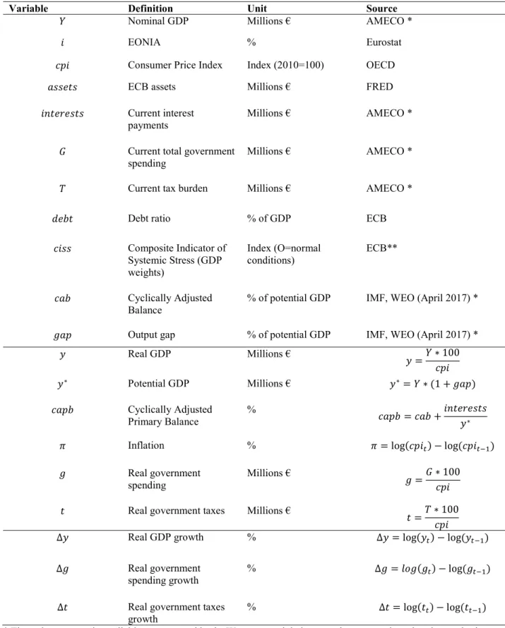
Table I.B. Data Sources, Definitions and Transformations (EMU)
Variable Definition Unit Source
𝑌 Nominal GDP Millions € AMECO *
𝑖 EONIA % Eurostat
𝑐𝑝𝑖 Consumer Price Index Index (2010=100) OECD
𝑎𝑠𝑠𝑒𝑡𝑠 ECB assets Millions € FRED
𝑖𝑛𝑡𝑒𝑟𝑒𝑠𝑡𝑠 Current interest
payments Millions € AMECO *
𝐺 Current total government
spending Millions € AMECO *
𝑇 Current tax burden Millions € AMECO *
𝑑𝑒𝑏𝑡 Debt ratio % of GDP ECB
𝑐𝑖𝑠𝑠 Composite Indicator of Systemic Stress (GDP weights) Index (O=normal conditions) ECB** 𝑐𝑎𝑏 Cyclically Adjusted
Balance % of potential GDP IMF, WEO (April 2017) *
𝑔𝑎𝑝 Output gap % of potential GDP IMF, WEO (April 2017) *
𝑦 Real GDP Millions € 𝑦 =𝑌 ∗ 100 𝑐𝑝𝑖 𝑦∗ Potential GDP Millions € 𝑦∗= 𝑌 ∗ (1 + 𝑔𝑎𝑝) 𝑐𝑎𝑝𝑏 Cyclically Adjusted Primary Balance % 𝑐𝑎𝑝𝑏 = 𝑐𝑎𝑏 + 𝑖𝑛𝑡𝑒𝑟𝑒𝑠𝑡𝑠 𝑦∗
𝜋 Inflation % 𝜋 = log(𝑐𝑝𝑖 ) − log (𝑐𝑝𝑖 )
𝑔 Real government
spending Millions € 𝑔 =
𝐺 ∗ 100 𝑐𝑝𝑖
𝑡 Real government taxes Millions €
𝑡 =𝑇 ∗ 100 𝑐𝑝𝑖
∆𝑦 Real GDP growth % ∆𝑦 = log(𝑦 ) − log (𝑦 )
∆𝑔 Real government
spending growth % ∆𝑔 = 𝑙𝑜𝑔(𝑔 ) − log (𝑔 )
∆𝑡 Real government taxes
growth % ∆𝑡 = log(𝑡 ) − log (𝑡 )
* These data were only available on an annual basis. We computed their quarterly averages by using the quadratic function in EViews.
25
Table II. Formal Specifications for the Estimated Models
Specification Vector of Endogenous var Vector of Exogenous var
Model 1 𝑌 = (∆𝑦 , ∆𝑐𝑎𝑝𝑏 , ∆𝑖 , 𝜋 ) 𝑋 = (∆𝑎𝑠𝑠𝑒𝑡𝑠 )
Model 2 𝑌 = (∆𝑦 , ∆𝑡 , ∆𝑔 , ∆𝑖 , 𝜋 ) 𝑋 = (∆𝑎𝑠𝑠𝑒𝑡𝑠 )
Model 3 𝑌 = (∆𝑦 , ∆𝑐𝑎𝑝𝑏 , ∆𝑖 , 𝜋 ) 𝑋 = (∆𝑎𝑠𝑠𝑒𝑡𝑠 , 𝑐𝑟𝑖𝑠𝑖𝑠 )
Model 4 𝑌 = (∆𝑦 , ∆𝑡 , ∆𝑔 , ∆𝑖 , 𝜋 ) 𝑋 = (∆𝑎𝑠𝑠𝑒𝑡𝑠 , 𝑐𝑟𝑖𝑠𝑖𝑠 )
Table III. Unit Root Tests
US EMU 𝑦 -0.52 -1.45 ∆𝑦 -4.49*** -3.57*** 𝑐𝑎𝑝𝑏 -1.70 -2.74* ∆𝑐𝑎𝑝𝑏 -3.95** -11.06*** 𝑡 -1.52 -1.22 ∆𝑡 -4.91*** -4.28*** 𝑔 -0.75 -0.45 ∆𝑔 -2.85* -3.83*** 𝑖 -2.65* -2.43 ∆𝑖 -4.45*** -4.85*** 𝜋 -7.66*** -3.11** 𝑔𝑎𝑝 -2.83* -2.02 ∆𝑔𝑎𝑝 -7.15*** -3.06** 𝑎𝑠𝑠𝑒𝑡𝑠 0.24 -0.27 ∆𝑎𝑠𝑠𝑒𝑡𝑠 -6.53*** -5.12***
Augmented Dickey-Fuller Test (ADF) containing a constant and up to 12 lags in its specification (Schwarz Info Criterion) on stationarity, where *, **, *** denotes that the null hypothesis that the variable contains a unit root is rejected at 10%, 5%, 1% significance level, respectively
26
27
28
Figure 3. Estimated IRFs to a fiscal shock from model 1 (US)
29
Figure 4. Estimated IRFs to a monetary shock from model 1 (US)
30
Figure 5. Estimated IRFs to a real government taxes shock from model 2 (US)
31
Figure 6. Estimated IRFs to a monetary shock from model 2 (US)
32
Figure 7. Estimated IRFs to a fiscal shock from model 1 (EMU)
33
Figure 8. Estimated IRFs to a monetary shock from model 1 (EMU)
34
Figure 9. Estimated IRFs to a real government taxes shock from model 2 (EMU)
35
Figure 10. Estimated IRFs to a monetary shock from model 2 (EMU)