A Work Project presented as part of the requirements for the Award of a Master’s Degree in Finance from the Nova School of Business and Economics
MEASURING SPILLOVER EFFECTS IN EURO AREA
EQUITY AND BOND MARKETS
Maria Inês Marques Gonçalves no.918
January of 2016
A Project carried out on the Master in Finance Program, under the supervision of: Professor Paulo M. M. Rodrigues
Abstract
Since its inception, the Eurozone has experienced significant financial integration. However, with the recent turbulent period, the dynamics of this integration may have changed. This study analyses the volatility spillovers from the US and aggregate Eurozone markets into ten Euro Area national equity and bond markets, using a regime-switching model with shifting shock sensitivities. The evidence confirms an increased impact of shock spillover intensity after the 2008 crisis in the equity market and a decrease of the same parameters for the bond market. In both markets, the overall impact of the Eurozone is greater when compared to the U.S.
Keywords: Regime-switching; Spillover effects; Eurozone
Acknowledgements
I thank Professor Paulo M. M. Rodrigues for his valuable guidance and support without whom the work would have never been accomplished. I also thank Professor Vladimir Otrachshenko for his suggestions and support in programming. At last, I would like to thank my family support.
1. Introduction
In 2008 a crisis of global proportions swept the financial markets across the world. From then on, the analysis of the linkages between the different financial markets has been a subject of increasing importance, since it plays an essential role in the study of the global financial crisis. The concern about financial contagion within its markets has become greater than ever before, particularly in Europe, due to the sovereign debt crisis that affected several countries in the European Monetary Union and demanded a financial rescue of some of the most affected ones: Greece, Portugal and Ireland.
In general, financial contagion defines a situation that is characterized by a transmission of instability from a specific market to one or several other markets or institutions (Constâncio, 2012). This issue affects policy-makers that must be aware of the effects that other markets have on their own country and use this knowledge to create fitting policies. It is therefore helpful to have a measure of impact of external markets, to know which ones are more significant and to understand the behavior of these spillovers during different economic periods (Louzis, 2013). Since the introduction of the Euro in 1999, the financial integration among the countries in the Eurozone has greatly increased, making them potentially more susceptible to contagion. Considering its special status of currency union without fiscal union that entails a limited ability to perform macroeconomic policies when these are needed, the Eurozone policy-makers should be particularly aware of the interdependencies among their countries. Thus, measuring and monitoring spillover effects across markets and asset classes has been a considerably important theme of research in financial studies over the last years.
Taking account of these facts, this report attempts to build a rigorous analysis of interdependences in the Eurozone and the effects of integration and globalization in both its
equity and bond markets. Using a model proposed by Baele (2005), a measure of time-varying shock spillover intensities for the last fifteen years, is presented.
This report is organized as follows: Section 2 summarizes previous research on the analysis of volatility spillovers across markets and on Markov-Switching models. Section 3 presents the methodology and explains the models used, whereas Section 4 displays and discusses the results. Finally, Section 5 reviews the results and its implications.
2. Literature Review
2.1 Financial Integration
Despite its undeniable benefits, financial globalization also has some drawbacks, specially related to the contagion that may occur in crises periods. Previous cases in history – such as the currency crises in Thailand in 97 which spread throughout East Asia or more recently the 2008 subprime crisis in the US – serve as prove of this argument. Several studies in empirical research also support this statement.
Starting with the work of Forbes and Rigobon (2002), who examined if cross-market correlation in stock market returns increased during crises periods, they define contagion as a significant increase in the linkages across markets after the occurrence of a shock in one country. Just like Calvo, Leiderman and Reinhart (1996) their study focuses on emerging economies. The latter find evidence that contagion occurs from the crisis country to the others and confirms that emerging markets are more prone to financial contagion.
In an analysis on the forces that determine volatility, Bekaert and Harvey (1997) find that in fully integrated markets, volatility is strongly influenced by world factors. Using a GARCH model for modeling conditional volatility, they find that volatility decreases when countries experience a liberalization.
It is confirmed that correlations across markets increase during turbulent periods and contagion occurs at that point in time (Papavassilliou, 2014). This evidence concerns financial agents that are trying to diversify their risk away, including in a portfolio several assets across different global markets. So even though globalization has allowed investors to spread their risk through diversification, the increase of its degree can, in contradiction, reduce the potential benefits of that strategy (Schmukler, 2004).
This has led to the analysis of the direction of spillovers and the correlation between different asset classes, especially relevant to portfolio allocation. Following the work of Ng (2000) evidence suggests that spillovers tend to move from developed to emerging markets and the last ones tend to be more integrated than the former. Baig and Goldfajn (1999) analyzed the Asian financial crisis of 97-98 conducting a cross-country correlation analysis among currencies, stock markets, interest rates and sovereign spreads. They have found evidence of contagion in the foreign exchange rate and tentative prove for the stock markets.
Relative to the European markets, a recent study by Papavassiliou (2014) proved that return correlation between stocks and sovereign bonds experienced an increase during the Greek debt crisis period and contagion occurred. Asgharian and Nossman (2011) analyze risk spillovers from the U.S. market and the regional market – constructed as a weighted average of all countries (under analysis) returns – to several European countries’ equity markets. They conclude that the regional market index has, in general, a higher contribution to the variances than the U.S.
Regarding the interaction of European and U.S. markets, Ehrmann, Fratzscher and Rigobon (2011) examine financial transmission across various assets, including stocks and bonds, using a multifactor framework to measure the volatility transmission. They conclude that even though
the strongest transmission of shocks at the international level occurs within asset classes, there is significant evidence of cross-market spillovers.
2.2 The Markov Switching Model
In this paper the main econometric model being used is the univariate Markov-Switching model of Hamilton (1989), also known as regime switching model. The specification of this model consists in the use of multiple structures to characterize the time series behavior in different regimes. In this way, allowing these structures to switch, allows more complex dynamic patterns to be captured. Variants of this model have been widely used in studies that tried to analyze economic as well as financial time series.
Currently, GARCH type models – as proposed by Engle (1982) and Bollerslev (1986) – are frequently used to model volatility in financial asset returns. However, these type of models have limitations when capturing the behavior of returns. Empirical research has provided evidence suggesting that the volatility of financial assets exhibits a type of persistence that cannot be captured by classical GARCH models, and previous research suggests that they tend to overestimate persistence in the conditional volatility. On the other hand, Markov-Switching models, allow parameters to change over time producing better volatility forecasts. (Bauwens, Preminger and Rombouts, 2006).
Cai (1994) and Hamilton and Susmel (1994) have combined the Markov-Switching with the ARCH model. Later, a combination of the GARCH model with the Markov-Switching was also introduced by Haas, Mittnik and Paolella (2004).
One of the advantages of the Markov-Switching approach is that it allows for the distinction between crisis periods and tranquil times. A crisis can be considered as a switch from a state characterized by low market pressure (“normal regime”) to another with a high market pressure
(“crisis regime”), i.e, time series experience jumps in the mean and in the volatility over time (Mandilaras and Bird, 2010).
Due to the possibility of differentiating between regimes, several studies have been using the regime-switching framework to investigate volatility behavior in financial markets. Gray (1996) models the conditional distribution of short-term interest rates using a “generalized regime-switching” structure that nests a GARCH (1, 1) model. Brunetti, Mariano, Scotti and Tan (2008) use a Markov-Switching GARCH model to analyze the exchange rate turmoil in Southeast Asia, differentiating between “turbulence” periods (of high exchange rate movements and high volatility) and “ordinary” periods (low exchange rate movements and low volatility). In the same line, Bialkowski, Bohl and Serwa (2006) use a Markov-switching framework to distinguish between calm and turmoil periods when analyzing financial spillovers from the U.S. to the U.K., the Japanese and German markets.
A Markov regime-switching framework is also used by Lopes and Nunes (2012) to study the case of the Portuguese escudo and the Spanish peseta during the EMS crisis period. Mandilaras and Bird (2010) perform an analysis of contagion in the Exchange Rate Mechanism of the EMS, using a Markov-Switching vector model with fixed transition probabilities to distinguish between crisis and non-crisis observations. They find that most of the foreign exchange market correlations increase during the crisis state.
Finally, a paper by Philippas and Siriopoulos (2013) use a spillover regime switching model, along with a conditional copula model, to investigate the contagion appetite of the recent debt crisis in Greece on six European Monetary Union bond markets. They find evidence of contagion appetite, dependent on macroeconomics imbalances and sovereign’s risk perception. They do not find however, an overall contagion effect from Greece to the others.
3. Methodology
The framework considered in this paper follows the work of Baele (2005) on volatility spillovers from aggregate European and U.S. markets to several local equity markets. In my research, I broaden the object of study to bond markets to describe the returns in the Euro Area and U.S. markets.
Following Ng (2000) and Baele (2005), the sources of shocks of unexpected returns are decomposed into three major components:
1) A domestic shock; 2) An European shock;
3) A global shock from the US;
The regime switching framework is incorporated in the spillover parameters by allowing them to switch between two states, in this case the crisis and the non-crisis states.
BIVARIATE MODEL FOR THE EU AND THE US
First, a bivariate model for the joint process of the weekly returns of the Euro Area and the U.S. stock and bond markets, 𝑟𝑡= [𝑟𝐸𝑈,𝑡 𝑟𝑈𝑆,𝑡]′, is specified as:
(1) [ 𝑟𝐸𝑈,𝑡 𝑟𝑈𝑆,𝑡] = [ 𝛼𝐸𝑈,0 𝛼𝑈𝑆,0] + [ 𝛼𝐸𝑈,1 𝛼𝐸𝑈,2 𝛼𝑈𝑆,1 𝛼𝑈𝑆,2] [ 𝑟𝐸𝑈,𝑡−1 𝑟𝑈𝑆,𝑡−1] + [ 𝜀𝐸𝑈,𝑡 𝜀𝑈𝑆,𝑡] = 𝛼0 + 𝐾𝜇𝑡−1+ 𝜀𝑡 (2) 𝜀𝑡ǀΩ𝑡−1~𝑁(0, 𝐻𝑡)
where 𝛼0 represents the vector of state dependent intercepts, 𝜀𝑡 is a vector of innovations, 𝜇 𝑡−1
is a vector of lagged 𝑟𝑖,𝑡 with state dependent coefficients 𝛼𝑖. The mean equation follows an AR(1) to account for possible serial correlation.
The model used is the Regime-Switching bivariate normal model, since it obtained the best results in the specification tests in Baele (2005) among all the models used, including the regime switching GARCH model.
The idea behind the Regime-Switching Normal model, is that we have two bivariate normal distributions that describe different sections of our time period. The distribution, depends on the time the process is in a specific regime, i.e.
(3) 𝑟𝑡ǀΩ𝑡−1 = {
𝑁(𝜇𝑡−1(𝑆𝑡= 1), 𝜎𝑡2(𝑆𝑡= 1))
𝑁(𝜇𝑡−1(𝑆𝑡= 2), 𝜎𝑡2(𝑆𝑡= 2))
}
where 𝑆𝑡 = 1 and 𝑆𝑡 = 2 are the two different states, one representing a high-volatility state and the other a low-volatility state. The mean equation is represented by 𝜇𝑡−1 and the variance by 𝜎𝑡2. The switching mechanism is therefore controlled by an unobservable state variable 𝑆
𝑡
that follows a two-state Markov-chain with transition matrix
P = [𝑝11 𝑝12 𝑝21 𝑝22]
and the constant transition probabilities are given by
𝑝11 = 𝑝𝑟𝑜𝑏(𝑆𝑡 = 1|𝑆𝑡−1= 1) and 𝑝22 = 𝑝𝑟𝑜𝑏(𝑆𝑡= 2|𝑆𝑡−1 = 2). Clearly, the transition probabilities satisfy 𝑝11 + 𝑝12 = 1. The transition matrix governs the random behavior of the state variable.
UNIVARIATE VOLATILITY SPILLOVER MODEL
For each country´s returns a univariate model is defined as
(4) 𝑟𝑖,𝑡 = 𝛽𝑖0+ 𝛽𝑖1𝑟𝑖,𝑡−1+ 𝛽𝑖2𝑟𝐸𝑈,𝑡−1+ 𝛽𝑖3𝑟𝑈𝑆,𝑡−1+ 𝜀𝑖,𝑡
As stated above, in the model developed by Ng (2000) and Baele (2005) the local unexpected returns have three sources of shocks, where two of them are the innovations provided by the U.S. and the EU returns. This model can be represented as,
(5) 𝜀𝑖,𝑡 = 𝑒𝑖,𝑡 + 𝛾𝑖𝐸𝑈(𝑆𝑖,𝑡𝐸𝑈)𝑒̂𝐸𝑈,𝑡+ 𝛾𝑖𝑈𝑆(𝑆𝑖,𝑡𝑈𝑆)𝑒̂𝑈𝑆,𝑡
where 𝑒̂𝐸𝑈,𝑡 and 𝑒̂𝑈𝑆,𝑡 are the residuals from the bivariate regime-switching model and 𝑒𝑖,𝑡 is an idiosyncratic shock following a conditional normal distribution with mean 0 and variance 𝜎𝑖,𝑡2. This conditional variance 𝜎𝑖,𝑡2 , is represented by a GJR-GARCH(1,1) process as,
(7) 𝜎𝑖,𝑡2 = 𝜓𝑖,1+ 𝜓𝑖,1𝑒𝑖,𝑡−12 + 𝜓𝑖,2𝜎𝑖,𝑡−12 + 𝜓𝑖,3𝑒𝑖,𝑡−12 𝐼{𝑒𝑖,𝑡−1< 0}
This model allows us to distinguish between the relative influence of the Euro Area and the US on each country´s market (Ng, 2000). However, to account for the possibility of Euro Area and US markets to be driven by common news, these innovations are orthogonalized, assuming that the Euro Area return shock is driven by a purely idiosyncratic shock and by the US return shock. These orthogonalized innovations are denoted by 𝑒̂𝐸𝑈,𝑡 and 𝑒̂𝑈𝑆,𝑡 and are computed using a Cholesky decomposition. Thus, (8) [𝑒̂𝐸𝑈,𝑡 𝑒̂𝑈𝑆,𝑡] = [ 1 −𝑘𝑡−1 0 1 ] [ 𝜀̂𝐸𝑈,𝑡 𝜀̂𝑈𝑆,𝑡] , with 𝑘𝑡 = 𝐻𝑒𝑢,𝑢𝑠,𝑡 𝐻𝑢𝑠,𝑡 , 𝜀𝑡ǀΩ𝑡−1~𝑁(0, 𝐻𝑡), 𝑒𝑡ǀΩ𝑡−1~𝑁(0, 𝛴𝑡),
With this modification, it is guaranteed that the Euro Area shock 𝑒̂𝐸𝑈,𝑡 is unrelated to the US shock 𝑒̂𝑈𝑆,𝑡.
The time variation spillover parameters 𝛾𝑖𝐸𝑈 and 𝛾𝑖𝑈𝑆are governed by two latent variables which allow for spillover intensities to assume two different values according to the correspondent state i.e.
(9) 𝛾𝑖,𝑡𝐸𝑈 = {𝑒𝑖,𝑡 + 𝛾𝑖,1
𝐸𝑈𝑒̂
𝐸𝑈,𝑡+ 𝛾𝑖,1𝑈𝑆 𝑒̂𝑈𝑆,𝑡 𝑖𝑓 𝑆𝑖,𝑡 = 1
𝑒𝑖,𝑡 + 𝛾𝑖,2𝐸𝑈𝑒̂𝐸𝑈,𝑡+ 𝛾𝑖,2𝑈𝑆 𝑒̂𝑈𝑆,𝑡 𝑖𝑓 𝑆𝑖,𝑡 = 2
In this model, to facilitate estimation, it is assumed that shock spillover intensities are ruled by the same forces, implying that 𝑆𝑖,𝑡𝐸𝑈 = 𝑆𝑖,𝑡𝑈𝑆 = 𝑆𝑖,𝑡. They follow the transition matrix
(10) Π𝑖 = [
𝑃𝑖 1 − 𝑃𝑖 1 − 𝑄𝑖 𝑄𝑖 ]
with 𝑃𝑖 = 𝑝𝑟𝑜𝑏(𝑆𝑖,𝑡 = 1|𝑆𝑖,𝑡−1 = 1) and 𝑄𝑖 = 𝑝𝑟𝑜𝑏(𝑆𝑖,𝑡 = 2|𝑆𝑖,𝑡−1 = 2).
To compute variance ratios it is assumed, based on Ng (2000) and Baele (2005), that local volatility ℎ𝑖,𝑡 can be decomposed as:
(11) 𝐸[𝜀𝑖,𝑡2 ǀ𝛺𝑡−1] = ℎ𝑖,𝑡 = 𝜎𝑖,𝑡2 + (𝛾̃𝑖,𝑡𝐸𝑈) 2
𝜎𝐸𝑈,𝑡2 + (𝛾̃𝑖,𝑡𝑈𝑆)2𝜎𝑈𝑆,𝑡2 ; (12) 𝐸[𝜀𝑖,𝑡2 ǀ𝛺𝑡−1] = (𝛾̃𝑖,𝑡𝐸𝑈)𝜎𝐸𝑈,𝑡2 ;
(13) 𝐸[𝜀𝑖,𝑡2 ǀ𝛺𝑡−1] = (𝛾̃𝑖,𝑡𝑈𝑆)𝜎𝑈𝑆,𝑡2 ;
The local variance 𝜎𝑖,𝑡2 follows a GJR-GARCH (1,1) specification and it is assumed that shocks
across countries are uncorrelated, 𝐸[𝑒𝑖,1𝑒𝑗,𝑡] = 0, ∀ 𝑖 ≠ 𝑗, and uncorrelated with the Euro Area and the US returns’ shocks. 𝛾̃𝑖,𝑡𝐸𝑈 and 𝛾̃𝑖,𝑡𝑈𝑆 represent the probability weighted shock spillover intensities obtained as
(14) 𝛾̃𝑖,𝑡𝐸𝑈 = 𝑝1,𝑡𝛾𝑖𝐸𝑈(𝑆𝑖,𝑡𝐸𝑈 = 1) + (1 − 𝑝1,𝑡)𝛾𝑖𝐸𝑈(𝑆𝑖,𝑡𝐸𝑈 = 2);
(15) 𝛾̃𝑖,𝑡𝑈𝑆 = 𝑝1,𝑡𝛾𝑖𝑈𝑆(𝑆𝑖,𝑡𝑈𝑆 = 1) + (1 − 𝑝1,𝑡)𝛾𝑖𝑈𝑆(𝑆𝑖,𝑡𝑈𝑆 = 2);
Finally, the ratios that measure the proportion of local variance that is explained, respectively, by the Euro Area and US shocks are
(16) 𝑉𝑅𝑖,𝑡𝐸𝑈 = (𝛾̃𝑖,𝑡𝐸𝑈) 2 𝜎𝐸𝑈,𝑡2 ℎ𝑖,𝑡
;
(17) 𝑉𝑅𝑖,𝑡𝑈𝑆 = (𝛾̃𝑖,𝑡𝑈𝑆) 2 𝜎𝑈𝑆,𝑡2 ℎ𝑖,𝑡 .4.1 Data and estimation
The dataset used consists of weekly returns from both the stock and the bond markets from ten Euro Area countries and two regional markets, the European market and the U.S. Stock market. Specifically, we use the Stoxx Europe 50 index for the European stock and the S&P500
index for the U.S. stock market (in euros). For the bond market, a series of weekly returns are computed from sovereign bond indices extracted from Bloomberg (bond yields on 10-year government bonds), using Germany as the proxy for the European bond market. The sample period for stock returns is from January 14, 2000 to October 30, 2015 over 15-years - which includes both the (2007-2009) subprime crisis and the recent European sovereign debt crisis. For the bond returns the sample period is somewhat shorter due to data availability for the U.S. sovereign bond index denominated in euros only from 2001. Asset prices are computed from the log differences of the closing prices excluding non-trading days (Friday-to-Friday). Weekly frequency is used to prevent issues with day-of-the-week and non-synchronous trading effects (Louzis, 2013).
Since the European index includes the countries under observation, we construct an European artificial index excluding the country itself, to avoid spurious spillovers. The methodology used to create the index is the one presented by Bekaert et al. (2005) and the weights are extracted from the Stoxx Euro 50 index fact sheet. The new indexes constructed are strongly correlated with the Euro index (above 98% correlation)1.
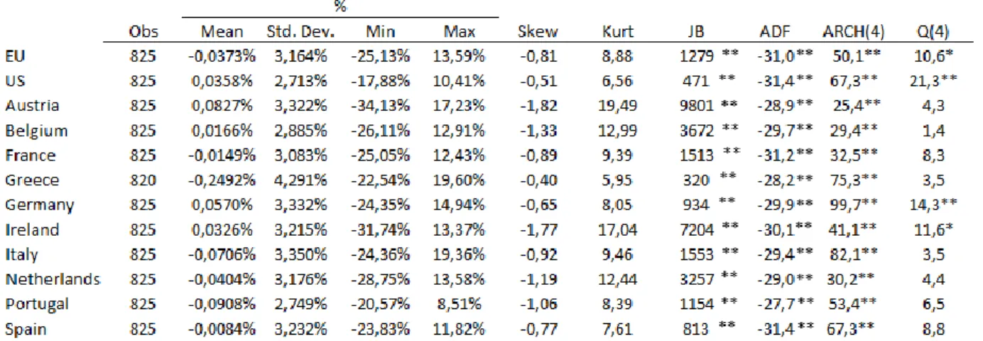
Before estimation of the models, I perform some tests on the weekly returns from the markets under study. Tables 1 and 2 present the summary statistics for the weekly stocks and bond returns, respectively, as well as the results of the tests on normality (Jarque-Bera test), autoregressive conditional heteroscedasticity (ARCH LM test) and autocorrelation (Portmanteau Q test for white noise). The mean returns on equity assume both negative (−0.2492% for Greece) and positive (0,0827% for Austria) values. For the bond returns, the values for the mean are all positive with the lowest value for Greece (0,0684%) and the highest for Germany (0,1596%). The most volatile market is Greece for both equity and bond markets, which is certainly a consequence of the crises experienced in this country from 2009 onwards.
1 Indexes are calculated as follows: ∑𝑘≠𝑖𝑤𝑘,𝑡𝑅𝑘,𝑡 ∑𝑘≠𝑖𝑤𝑘,𝑡
As expect from financial assets, all countries present excess kurtosis and negative skewness, and the Jarque-Bera test is significant, indicating a rejection of normality. The presence of excess kurtosis shows that extreme values (excessive gains and losses) are more frequent in this series than would be expected in a normal distribution. The ARCH test shows that for both stock and bond data, returns exhibit conditional heteroscedasticity and the Q test reveals significant autocorrelation in most markets. Therefore, we should model returns using an ARCH or GARCH model to account for this characteristics.
Table 1. Summary statistics for the stock returns
Table 3. Estimation Results for the Bivariate Regime-Switching model for the EU and US Stock Returns
4.2 Empirical Results
4.2.1 Bivariate model for the EU and the US
Table 3 presents the estimation results of the bivariate regime-switching model previously introduced.
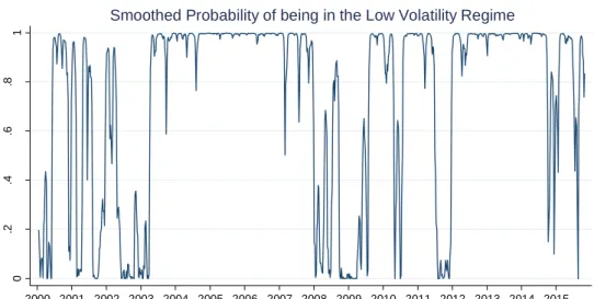
These results show a separation of states based on the levels of volatility. Eurozone and US equity markets are in high and low volatility states at the same time. The results also suggest that returns are insignificant or negative in the high volatility state (state 2), with more evidence for significance in the low volatility state (state 1). Using a graph to plot the smoothed probabilities that both the Eurozone and US equity markets are jointly in the low volatility state, we can observe that in the years previous to the financial crisis of 2008 these markets were mainly in the low volatility state. The switch occurred after that period with slumps at the most critical years of the crisis, 2009 with the propagation of the crisis in Europe and 2010 with the bailouts of some European countries: Greece (2010), Ireland (2010) and Portugal (2011). In 2012, Greece was provided with a second bailout package and defaulted on its debt and due to political instability, the hypothesis of a “Grexit” began to be advanced, a speculation of a possible exit of Greece from the Euro. All these occurrences are likely to lead to an increase in market volatility and coincide with the high volatility period.
Table 4. Estimation Results for the Bivariate Regime-Switching for German and US Bond Returns
4.2.2 Bivariate model for Germany and US
The estimation results for the bivariate regime-switching normal model for the bonds are presented in Table 4.
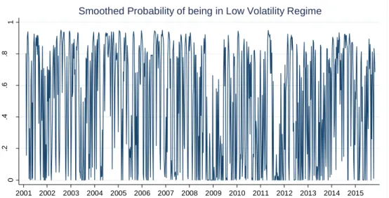
Based on these results, the conclusions are the same as those from the equity market. Both the Eurozone – using Germany Bonds – and the US bond returns are in the high volatility state at the same time and returns seem also higher in the low volatility state. Nonetheless, the figure that plots the joint probability of both markets being in the low volatility state is much different from before. 0 .2 .4 .6 .8 1 2000 2001 2002 2003 2004 2005 2006 2007 2008 2009 2010 2011 2012 2013 2014 2015
Figure 2. Smoothed Probability of being in the Low Volatility Regime for Bond Returns
For the bond market, there is a constant switch between the period of low and high volatility. The duration of each regime is much lower too, with 2.71 time periods for state 1 and 2.90 time periods for state 2, whereas for the stock returns not only was the duration of each regime higher, but also the difference between the duration of each regime was more significant. (Regime1:26.06 time periods; Regime2:9.31 time periods).
This could be due to the fact that volatility in bond returns is not only lower, but less influenced by common news, with investors doing a proper distinction between countries and taking country specific risk more into account. Also, the difference between the level of volatility in states 1 and 2 is lower when compared with the equity markets, in which the distinction between regimes is less evident.
4.2.3 Univariate Spillover Model
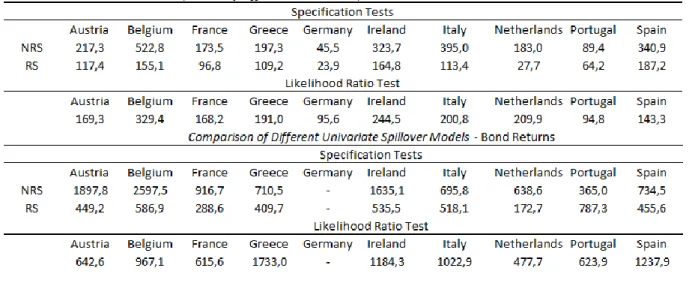
To assess the differences between the univariate model with regime switching spillovers and a model with constant spillover parameters, a joint test for normality in the standardized residuals is used, testing the null hypothesis of mean zero, unit variance, no autocorrelation up to order 4, no skewness and no excess kurtosis. Even though both models produce large test statistics, for all countries, the model with regime-switching spillovers produces the lowest test
0 .2 .4 .6 .8 1 2001 2002 2003 2004 2005 2006 2007 2008 2009 2010 2011 2012 2013 2014 2015
Table 5. Comparison of Different Spillover Models Stock and Bond Returns
statistics, suggesting that the regime-switching model is more suitable to model the mean and variance of local returns (Baele, 2005). A Likelihood ration test is also performed to analyze whether models are statistically different from each other. To perform the test, a model was perform the likelihood and therefore could be used as an indicator of significance. In all countries, the single regime model is rejected in favor of the two regime switching model, serving as evidence that regime switches should be taken into account.
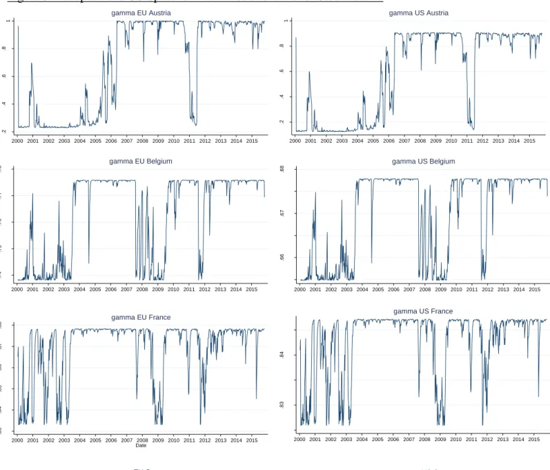
4.2.4 Results on Regime switching spillover effects
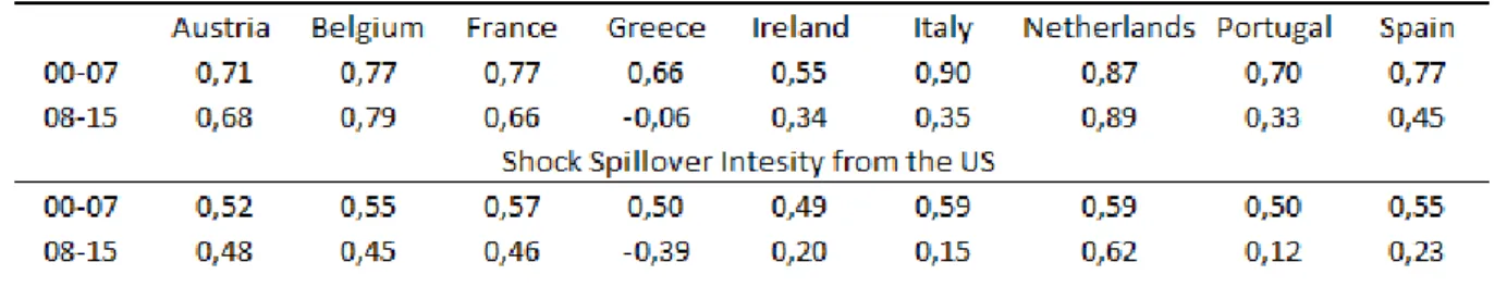
Table 6 presents the results of the shock spillover intensities. To have a better understanding of the evolution of these intensities over time and with respect to the crises period, the results for two time periods are presented: the “pre-crises” period, from 2000 to 2007 – and 2001 to 2007 in the bond market case -, and the crises and its aftermath period from 2008 to 2015. The evolution of shock spillover is also represented in Figures 3 and 4 (please see appendix)
For stocks, in the majority of countries, the sensitivity to EU shocks is greater than to US shocks, with the exception of the Germany, Ireland and Netherlands. This could be related to the higher interconnections of these economies with the US market.
Regarding the evolution of the sensitivity to shocks, it has increased with respect to the “pre-crisis” period in all countries, with the exception of Germany, the Netherlands and France. Surprisingly, in the two former economies (Germany and the Netherlands) the sensitivity to both EU and US shocks has slightly decreased whereas France presented roughly the same values over time. This unexpected result is verified in three of the strongest economies in the Eurozone and could be an indicator of their relative good performance in contrast with the other countries markets in turbulent times. At the same time, the countries where that increase is more noticeable include the ones more affected by the crisis: Portugal, Greece and Italy.
In the case of bonds, the difference of impact of the Eurozone (represented by the German Bond index) is even more significant when compared to the US. The evolution of its values over time is opposite to the stocks behavior, with the decrease of the sensitivity to shocks in the crises period and after that, with the exception of the Netherlands and Belgium. This could result from the change in investor’s perception about the bonds in the Eurozone. Before the crisis, Euro Area countries sovereign bonds were seen as similar investments in terms of risk. After the
Table 8. Time-varying spillover effects for the Bond Market
sovereign debt crises exposed the true fiscal situation of some periphery countries, the yields on these countries increased relative to the German benchmark, reflecting the different levels of credit risk associated to each country.
The next two Tables, present the proportion of total return variance that can be attributed to EU and US shock spillovers. Again, the proportion of variance attributed to EU shocks is dominant, and is on average higher for the following countries: France, Portugal, Greece and Spain. For bonds, the EU is still the dominant force, but it is important to notice that Portugal, Greece, Italy and Spain present now the lowest proportions of variance, which could be an evidence of the divergence that the bond market experienced in the Eurozone with the sovereign debt crisis. Since we are using the German bonds as a proxy, the proportion of variance explained by this asset is lower in the countries with the highest spread.
Table 9. Variance Proportions accounted for the EU and US stock markets
5. Conclusion
The purpose of this work, is to measure and understand the level of interdependence in a strongly integrated market like the Eurozone. Both equity and bond markets are analyzed and Eurozone shocks intensity is compared to global shocks, using the US as a proxy. The time period under study which includes both a “calm” period and a “turbulent” period, with the 2008 financial crises and the European sovereign debt crises, justifies the use of a regime switching framework to account for the behavior of the returns in the different time periods.
Based on the empirical findings, both regional (Eurozone) and world factors have an important impact on market volatility in the countries under analysis, with stronger influence from the Eurozone. For equity markets, in general, these factors have experienced an increase in its intensity, especially remarkable after the 2008 crises period. Evidence suggests, that a country’s economic performance may be linked to the intensity of shock spillovers, with stronger economies observing a decrease in its values.
Regarding the bond markets, the Eurozone impact compared to the US is even more significant, even though its behavior over time is the opposite of that of the stock market. Spillover intensities decrease after the crisis of 2008, which is seen as a consequence of the increase in the spreads of these countries with regards to the German bonds, which are used as a Euro market proxy.
These findings suggest an increase in market integration in the equity market, especially evident with the 2008 crisis, which could contribute to the loss of potential diversification. The result also confirms the importance of the Eurozone market on each member’s economy, revealing an increase in its importance also when compared with previous studies before the introduction of the Euro. In the bond market, they also suggest a decrease in integration,
possibly due to the sovereign debt crisis that created divergence in perception of investors’ country specific risk.
Specification and a likelihood ratio tests offer evidence for the accuracy of the regime switching model when compared to the non-regime-switching, which provides an advantage in this analysis. Disadvantages of this study are related to assumption of common regime switches between the Eurozone and the US market. This assumption implies that forces that govern shock spillover intensities are the same. This restricts the shifts in the shock spillover intensities, creating a prediction that may not be true. Another drawback may be the use of indexes that exclude the country under observation as they may not be as accurate, since they were extracted from Bloomberg and created based on given weights. Besides these factors, the use of Germany as the Euro Area proxy for bond returns is not a perfect substitute for Eurobonds especially after the sovereign debt crisis that created divergence in bond markets in this region.
In the future, it would be interesting to extend the analysis to countries that more recently joined the monetary union as well as to measure the correlations between the different markets.
References
Asgharian, Hossein and Marcus Nossman. 2011. "Risk contagion among international
stock markets." Journal of International Money and Finance, 30(1): 22-38
Baig, Taimur and Ilan Goldfajn. 1999. “Financial Market Contagion in the Asian Crisis”,
IMF Staff Papers, 46 (2): 167-195
Bauwens, Luc, Arie Preminger and Jeroen V.K. Rombouts. 2006. "Regime Switching
Garch Models." Ben-Gurion University of the Negev, Department of Economics, Working Papers 0605
Białkowski, Jedrzej, Martin T. Bohl, and Dobromił Serwa. 2006. “Testing for Financial
Spillovers in Calm and Turbulent Periods.” Quarterly Review of Economics and Finance 46(3): 397–412.
Bekaert, Geert, and Campbell R. Harvey. 1997. “Emerging Equity Market Volatility.”
Journal of Financial Economics, 43(1): 29–77.
Bekaert, Geert, Campbell R. Harvey, and Angela Ng. 2005. “Market Integration and
Contagion.” Journal of Business, 78(1): 39-69
Białkowski, Jedrzej, Martin T. Bohl, and Dobromił Serwa. 2006. “Testing for Financial
Spillovers in Calm and Turbulent Periods.” Quarterly Review of Economics and Finance, 46(3): 397–412.
Bollerslev, Tim. 1986. “Generalized autoregressive conditional heteroskedasticity.” Journal
of Econometrics, 31: 307–27.
Brunetti, Celso, Roberto S. Mariano, Chiara Scotti and Augustine H.H. Tan. 2008.
“Markov Switching GARCH Models of currency turmoil in Southeast Asia.” Emerging
Cai, Jun. 1994. “A Markov Model of Switching-Regime ARCH.” Journal of Business &
Economic Statistics, 12(3): 309–16.
Calvo, Guillermo A., Leonardo Leiderman and Carmen M. Reinhart. 1996. The Journal
of Economic Perspectives, 10(2): 123-139.
Chen, Ruquan. 2009. “Volatility and Correlation in Financial Markets: Econometric Modeling
and Empirical Pricing.” Phd diss. London School of Economics
Christiansen, Charlotte. 2007. “Volatility-Spillover Effects in European Bond Markets.”
European Financial Management, 13(5): 923–48.
Constâncio, Vitor. 2012. “Contagion and the European Debt Crisis.” Financial Stability
Review, (16): 109–21.
Ehrmann, Michael, Marcel Fratzscher and Roberto Rigobon. 2011. “Stocks, Bonds and
Exchange Rates: Measuring International Financial Transmission.” Journal of Applied
Econometrics, 26: 948-974
Engle, Robert F. 1982. “Autoregressive Conditional Heteroscedasticity with Estimates of the
Variance of United Kingdom Inflation.” Econometrica, 50(4): 987-1007
Forbes Kristin J. and Roberto Rigobon. 2002. “No Contagion, Only Interdependence:
Measuring Stock Market Comovements.” The Journal Of Finance, 57(5): 2223–2261.
Gray, Stephen F. 1996. “Modeling the conditional distribution of interest rates as a
regime-switching process”. Journal of Financial Economics, 42(1): 27-62.
Haas, Markus, Stefan Mittnik and Mark S. Paolella. 2004. “Mixed normal conditional
heteroscedasticity”. Journal of Financial Econometrics, 2, 211–250
Hamilton, James D. 1989. “A New Approach to the Economic Analysis of Nonstationary
Hamilton, James D. and Raul Susmel. 1994. “ARCH and Changes in Regime.” Journal of
Econometrics, 64: 307-333
Mandilaras, Alex and Graham Bird. 2010. "A Markov switching analysis of contagion in the
EMS," Journal of International Money and Finance, 29(6): 1062-1075
Mário, José, and Luís C. Nunes. 2012. “A Markov regime switching model of crises and
contagion: The case of the Iberian countries in the EMS”. Journal of Macroeconomics, 34: 1141–1153
Ng, Angela. 2000. “Volatility Spillover Effects from Japan and the US to the Pacific–Basin.”
Journal of International Money and Finance, 19(2): 207–33
Papavassiliou, Vassilios G. 2014. “Cross-Asset Contagion in Times of Stress.” Journal of
Economics and Business 76: 133–39.
Papavassiliou, Vassilios G. 2014. “Financial Contagion during the European Sovereign Debt
Crisis: A Selective Literature Review.” Crisis Observatory, ELIAMEP, Hellenic Foundation for European & Foreign Policy, Research Paper No 11
Philippas, Dionisis, and Costas Siriopoulos. 2013. “Putting the ‘C’ into Crisis: Contagion,
Correlations and Copulas on EMU Bond Markets.” Journal of International Financial Markets,
Institutions and Money, 27: 161–76.
Schmukler, Sergio L. 2004. "Financial globalization: gain and pain for developing countries."
.4 5 .5 .5 5 .6 .6 5 2000 2001 2002 2003 2004 2005 2006 2007 2008 2009 2010 2011 2012 2013 2014 2015 gamma US Greece
Figure 3- European and US Spillover Intensities over time for Stock returns
.2 .4 .6 .8 1 2000 2001 2002 2003 2004 2005 2006 2007 2008 2009 2010 2011 2012 2013 2014 2015 gamma US Austria .2 .4 .6 .8 1 2000 2001 2002 2003 2004 2005 2006 2007 2008 2009 2010 2011 2012 2013 2014 2015 gamma EU Austria .7 4 .7 5 .7 6 .7 7 .7 8 2000 2001 2002 2003 2004 2005 2006 2007 2008 2009 2010 2011 2012 2013 2014 2015 gamma EU Belgium .6 5 5 .6 6 .6 6 5 .6 7 .6 7 5 .6 8 2000 2001 2002 2003 2004 2005 2006 2007 2008 2009 2010 2011 2012 2013 2014 2015 gamma US Belgium .8 3 .8 4 .8 5 .8 6 .8 7 .8 8 2000 2001 2002 2003 2004 2005 2006 2007 2008 2009 2010 2011 2012 2013 2014 2015 Date gamma EU France .8 2 5 .8 3 .8 3 5 .8 4 .8 4 5 2000 2001 2002 2003 2004 2005 2006 2007 2008 2009 2010 2011 2012 2013 2014 2015 gamma US France .6 .7 .8 .9 1 2000 2001 2002 2003 2004 2005 2006 2007 2008 2009 2010 2011 2012 2013 2014 2015 gamma EU Germany .7 5 .8 .8 5 .9 .9 5 2000 2001 2002 2003 2004 2005 2006 2007 2008 2009 2010 2011 2012 2013 2014 2015 gamma US Germany .7 5 .8 .8 5 .9 2000 2001 2002 2003 2004 2005 2006 2007 2008 2009 2010 2011 2012 2013 2014 2015 gamma EU Greece
.4 5 .5 .5 5 .6 .6 5 2000 2001 2002 2003 2004 2005 2006 2007 2008 2009 2010 2011 2012 2013 2014 2015 .6 .6 5 .7 .7 5 .8 .8 5 2000 2001 2002 2003 2004 2005 2006 2007 2008 2009 2010 2011 2012 2013 2014 2015 .7 .8 .9 1 1 .1 2000 2001 2002 2003 2004 2005 2006 2007 2008 2009 2010 2011 2012 2013 2014 2015 gamma EU Italy .7 .7 5 .8 .8 5 2000 2001 2002 2003 2004 2005 2006 2007 2008 2009 2010 2011 2012 2013 2014 2015 gamma US Italy .7 .7 5 .8 .8 5 .9 .9 5 2000 2001 2002 2003 2004 2005 2006 2007 2008 2009 2010 2011 2012 2013 2014 2015 gamma EU Netherlands .8 4 5 .8 5 .8 5 5 .8 6 2000 2001 2002 2003 2004 2005 2006 2007 2008 2009 2010 2011 2012 2013 2014 2015 gamma US Netherlands .5 .6 .7 .8 .9 2000 2001 2002 2003 2004 2005 2006 2007 2008 2009 2010 2011 2012 2013 2014 2015 gamma EU Portugal .3 .4 .5 .6 .7 2000 2001 2002 2003 2004 2005 2006 2007 2008 2009 2010 2011 2012 2013 2014 2015 gamma US Portugal .9 4 .9 6 .9 8 1 2000 2001 2002 2003 2004 2005 2006 2007 2008 2009 2010 2011 2012 2013 2014 2015 gamma EU Spain .6 9 .7 .7 1 .7 2 .7 3 .7 4 2000 2001 2002 2003 2004 2005 2006 2007 2008 2009 2010 2011 2012 2013 2014 2015 gamma US Spain
.6 2 .6 4 .6 6 .6 8 .7 .7 2 2001 2002 2003 2004 2005 2006 2007 2008 2009 2010 2011 2012 2013 2014 2015 gamma GER Austria
.4 2 .4 4 .4 6 .4 8 .5 .5 2 2001 2002 2003 2004 2005 2006 2007 2008 2009 2010 2011 2012 2013 2014 2015 gamma US Austria .7 7 .7 8 .7 9 .8 2001 2002 2003 2004 2005 2006 2007 2008 2009 2010 2011 2012 2013 2014 2015 gamma GER Belgium
.4 .4 5 .5 .5 5 2001 2002 2003 2004 2005 2006 2007 2008 2009 2010 2011 2012 2013 2014 2015 gamma US Belgium .5 5 .6 .6 5 .7 .7 5 .8 2001 2002 2003 2004 2005 2006 2007 2008 2009 2010 2011 2012 2013 2014 2015 gamma GER France
.3 5 .4 .4 5 .5 .5 5 .6 2001 2002 2003 2004 2005 2006 2007 2008 2009 2010 2011 2012 2013 2014 2015 gamma US France -. 2 0 .2 .4 .6 2001 2002 2003 2004 2005 2006 2007 2008 2009 2010 2011 2012 2013 2014 2015 gamma GER Greece
-. 5 0 .5 2001 2002 2003 2004 2005 2006 2007 2008 2009 2010 2011 2012 2013 2014 2015 gamma US Greece
.3 .3 5 .4 .4 5 .5 .5 2001 2002 2003 2004 2005 2006 2007 2008 2009 2010 2011 2012 2013 2014 2015 .1 .2 .3 .4 .5 2001 2002 2003 2004 2005 2006 2007 2008 2009 2010 2011 2012 2013 2014 2015 .2 .4 .6 .8 1 2001 2002 2003 2004 2005 2006 2007 2008 2009 2010 2011 2012 2013 2014 2015 gamma GER Italy
0 .2 .4 .6 2001 2002 2003 2004 2005 2006 2007 2008 2009 2010 2011 2012 2013 2014 2015 gamma US Italy .2 .3 .4 .5 .6 .7 2005 2006 2007 2008 2009 2010 2011 2012 2013 2014 2015 gamma GER Portugal
.1 .2 .3 .4 .5 .6 2001 2002 2003 2004 2005 2006 2007 2008 2009 2010 2011 2012 2013 2014 2015 gamma US Spain .4 .5 .6 .7 .8 2001 2002 2003 2004 2005 2006 2007 2008 2009 2010 2011 2012 2013 2014 2015 gamma GER Spain
.8 6 .8 8 .9 .9 2 2001 2002 2003 2004 2005 2006 2007 2008 2009 2010 2011 2012 2013 2014 2015 gamma GER Netherlands
.5 8 .6 .6 2 .6 4 .6 6 2001 2002 2003 2004 2005 2006 2007 2008 2009 2010 2011 2012 2013 2014 2015 gamma US Netherlands 0 .1 .2 .3 .4 .5 2005 2006 2007 2008 2009 2010 2011 2012 2013 2014 2015 gamma US Portugal