As for other controls, they all come from the WDI, as follows: population growth, imports and exports of goods and services (in of GDP) – whose sum gives us the trade openness - and

(1)

Carlos Pestana Barros & Nicolas Peypoch

A Comparative Analysis of Productivity Change in Italian and Portuguese Airports

WP 006/2007/DE _________________________________________________________

António Afonso & João Tovar Jalles

Fiscal Volatility, Financial Crises and Growth

WP 06/2012/DE/UECE _________________________________________________________

De pa rtme nt o f Ec o no mic s

W

ORKING

P

APERS

ISSN Nº 0874-4548

School of Economics and Management

(2)

Fiscal Volatility, Financial Crises and Growth

António Afonso

$ #

and João Tovar Jalles

#

January 2012

Abstract

We use a panel of developed and emerging countries for the period 1970-2008 to assess how fiscal policy volatility and financial crises affect growth. We find that economic growth is lower in the presence of more volatile fiscal policy. Moreover, with a financial crisis government spending is stickier than revenue.

JEL: C23, E62, H50.

Keywords: growth, fiscal volatility, crises, panel analysis.

1. Introduction

Fiscal volatility is an important issue concerning fiscal policy and its effect on growth. From a theoretical point of view, restrictions on government expenditure volatility may have both positive and negative effects on long-run growth. With regard to government spending in particular, the theoretical pendulum appears to sway towards the conventional wisdom, that it may be a source of economic instability. On the one hand, governments can smooth out the business cycle fluctuations by the use of discretionary changes in fiscal policy1 and by the use of automatic stabilizers (e.g., Sachs and Sala-i-Martin, 1992; von Hagen, 1992; Afonso and Furceri, 2008). Therefore, fiscal policy may positively affect private investment and long-run growth. On the other hand, fiscal policy itself might be a source of business cycle fluctuations and exacerbate (undesirably) macroeconomic volatility, e.g., in case of pro-cyclical measures. In addition, given the difficulties in implementing sustainable fiscal policies, it is worthwhile assessing the impact of fiscal volatility on economic activity.

$_{ISEG/UTL - Technical University of Lisbon, Department of Economics; UECE – Research Unit on Complexity and}

Economics. UECE is supported by FCT (Fundação para a Ciência e a Tecnologia, Portugal), email: aafonso@iseg.utl.pt.

#_{European Central Bank, Directorate General Economics, Kaiserstraße 29, D-60311 Frankfurt am Main, Germany. email:}

antonio.afonso@ecb.europa.eu.

_{University of Aberdeen, Business School, Edward Wright Building, Dunbar Street, AB24 3QY, Aberdeen, UK. email:}

j.jalles@abdn.ac.uk

#_{European Central Bank, Directorate General Economics, Kaiserstraße 29, D-60311 Frankfurt am Main, Germany. email:}

joao.jalles@ecb.europa.eu.

1

(3)

2

Since changes in fiscal policy may be linked to financial crises, which by themselves have a detrimental effect on macroeconomic outcomes and macro (and fiscal) volatility, it is important to clarify the effect such disruptive events have on the fiscal-growth relationship. This idea is also related to the degree of responsiveness and persistence of fiscal policy to macroeconomic conditions (Afonso et al. 2010). While extraordinary fiscal measures have contributed to reduce the real impact of the recent crisis, they also have increased the burden of public debt and the size of (implicit) fiscal contingent liabilities, raising concerns about fiscal sustainability in a number of countries, all of which further damper growth prospects.

Section 2 presents the dataset and methodology. Section 3 discusses the empirical results. The last section concludes.

2. Methodology and data

In the context of a neoclassical growth model we use the following empirical specification to assess the linkages between fiscal policy (volatility and financial crises) and growth.

it i t it it it io

it it

it y y x G S

y  _₁  ₀ ₁      (1) where i (i=1,…,N) denotes the country, t (t=1,…,T) indicates the period, y_it y_it_₁represents the growth rate of real GDP per capita; yi₀is the initial value of real GDP per capita; xit is a vector of control variables (population growth, investment, education and trade openness);

it

G is a fiscal policy-related variable, either total government revenues or expenditures; S_it is a vector of either fiscal volatility measures or financial crises dummies interacted with fiscal variables; i, tcorrespond to the country-specific and time effects, respectively. Finally, it is a column vector of some unobserved zero mean white noise-type satisfying the standard assumptions.   , ₀, ₁, and  are unknown parameters.

Our dependent variable, the growth rate of real GDP per capita, comes from the World Bank’s Word Development Indicators (WDI). Fiscal variables come from the WDI, the IMF’s International Financial Statistics (IFS) and Easterly’s (2001) data. They comprise of the Total Government Revenue and Total Government Expenditure (both in % of GDP). With respect to human capital proxies we rely on the average years of schooling for the population over 25 years old from the international data on educational attainment by Barro and Lee (2010).2 As for other controls, they all come from the WDI, as follows: population growth, imports and exports of goods and services (in % of GDP) – whose sum gives us the trade openness - and

2

(4)

gross fixed capital formation (proxying for investment). We measure fiscal volatility by taking the standard deviation of both total government revenues and expenditures over each 5-year period and we then include these in our regression equation (we simultaneously include each of the two government variables of interest with one volatility measure). Financial crises dummies come from Leaven and Valencia’s (2010) publicly available database. We interact expenditures and revenues with banking, debt and currency dummies as additional regressors and include one at a time.

Turning to the econometric techniques, cross-country regressions are usually based, in this context, on average values of fiscal variables and growth over long time periods. However, for long time spans, the level of government spending is likely to be influenced by demographics, particularly by an increasing share of elderly people. Therefore, a simultaneity issue arises. Moreover, problems such as endogeneity, both in terms of government spending and tax policies, and inefficiency, due to the discarding of information on within-country variation, can come up. Resorting to panel data can overcome (some of) these problems, and has other advantages. Specifically, we focus mainly on combined cross-section time-series regressions using cumulative 5-year non-overlapping averages to smooth the effects of short-run fluctuations. We short-run within fixed-effects as a benchmark model despite being aware of the econometric IV-related problems associated with this method in the context of fiscal policy and growth. Given that technological change occurs over time, a time index is a logical way to control for the effect of technological progress on the evolution of per capita GDP growth. However, the effect of technological change on output growth would likely not be well captured by a simple time trend that assumes a constant effect over time. Therefore, non-linear effects of technological change on output growth are allowed for by using individual year indicator dummies in our estimated panel models.3

One needs to address the potential endogeneity problem of right-hand side regressors and while country-specific fixed effects might capture some of the omitted variables (if we miss out an important variable it not only means our model is poorly specified it also means that any estimated parameters are likely to be biased), it does not solve the problem and we may get may get biased coefficient estimates. Therefore, we also estimate (1) using Generalised Methods of Moments (GMM). The first-differenced GMM estimate can be poorly behaved if the time series are persistent. This problem can get very serious in practice and authors like

3

(5)

4

Bond, Hoeffler and Temple (2001) suggest the use of a more efficient GMM estimator, the system estimator, to exploit stationarity restrictions.4

3. Empirical Results

Looking at Table 1, we find that volatility of both expenditures and revenues is detrimental to output growth, in line with the findings of Afonso and Furceri (2010). As a robustness exercise other volatility measures were computed, more specifically, we applied the Hodrick-Prescott (HP), the Baxter-King (BK) and Christiano-Fitzgerald random walk (CFRW) filters to the levels of total government expenditures and revenues in order to extract their cyclical components. We then took the standard deviation over each 5-year period of the extracted cyclical components. For reasons of parsimony results with alternative filtering procedures are available upon request but conclusions are qualitatively similar.

[Table 1]

Additionally, we find evidence that total government revenues affect growth negatively (as in Plosser, 1992) in emerging economies (Table 2). A similar general conclusion also applies to government spending whose negative and significant coefficient is robust across full and OECD samples (Fölster and Henrekson, 1999).5 The detrimental effect of revenue volatility seems to be much larger for OECD countries than for emerging economies, while the negative effect of spending volatility is rather similar across country groups, which is consistent with others’ results (e.g., Aghion et al., 2006). Running a system GMM estimator instead does not alter the main findings.

[Table 2]

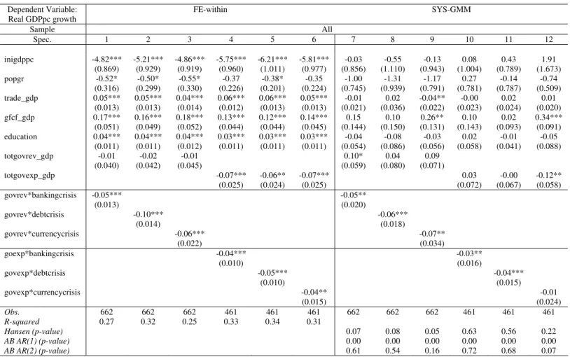
Turning to the effect of financial (bank, debt, and currency) crises, our results in Table 3 show that for the full sample government revenue appears to be statistically insignificant6 but when interacted with any type of financial crisis there is then an adverse effect for output growth, associated with revenue losses in the collection processes, which can be related with lower economic activity.

Moreover, the magnitude of the interaction terms when revenue is considered is higher than when government expenditures are used, in other words, with a financial crisis

4

Although stationarity of averages of investment and population growth rates are quite consistent with the Solow growth model, constant means of per capita GDP series are clearly not. Fortunately, also here, the inclusion of the time dummies solves the problem without violating the validity of the additional moment restrictions used by the system GMM estimator. In the type of convergence regressions to be analysed, the succession of time dummies can be interpreted as the evolution of common TFP over time.

5

Including a quadratic term as an additional regressor in our specifications, for both expenditures and revenues, does not provide meaningful estimated coefficients (not shown for parsimony).

6

(6)

government spending is stickier than revenue. This finding is corroborated by Afonso et al. (2010) who find that government revenue reacts relatively more to macro conditions (and seem to be less persistent). Government expenditures keep their statistically negative coefficients and the detrimental effects in output growth are further deepened when crisis take place and governments have to incur in increased socially-related expenditure facing the aftermath of economic busts. From a policy perspective, the fact that fiscal policy is rather persistent (particularly expenditures) implies that the fiscal authorities have less leeway to curb spending behaviour. For the OECD sub-group results (not shown) are similar but only banking and debt crisis more consistently affect growth negatively when interacted with either government revenues or expenditures.

[Table 3]

Finally, Beetsma and Giuliodori (2010) reported on the existence of fiscal policy interdependence for EU countries. In this context, we apply Pesaran’s (2004) CD test for the OECD sub-sample and find a statistic of 15.26, corresponding to a p-value of zero (the null hypothesis is of cross-sectional independence).7 We re-run the main regressions with Dricoll-Kraay (1998) robust standard errors – this non-parametric technique assumes the error structure to be heteroskedastic, autocorrelated up to some lag and possibly correlated between groups. Our results, not presented for reasons of parsimony, are in line with previous findings.

4. Conclusion

In a panel of developed and emerging countries for the period 1970-2008 we assessed how fiscal policy volatility and financial crises impact on growth, via the use of the standard deviation over each 5-year period of the extracted cyclical components of government spending and revenue. We find that economic growth is lower in the presence of volatile fiscal policy. Therefore, the implementation of smoother fiscal policies helps creating a friendlier and stable growth environment, via, for instance, more stable tax codes that allow private investors to plan better in the medium term.

Moreover, government revenue volatility seems to be larger for OECD countries than for emerging economies, while the negative effect of spending volatility is rather similar across country groups. In addition, with a financial (bank, debt, and currency) crisis government spending is stickier than revenue. Hence, in the context of such crisis, the effects on fiscal imbalances tend to be magnified, due to higher revenue drops, which can be seen as also highlighting the relevance of automatic stabilisers.

(7)

6 References

1. Afonso, A., Furceri, D. (2008), “EMU Enlargement, Stabilisation Costs and Insurance Mechanisms”, Journal of International Money and Finance, 27 (2), 169-187.

2. Afonso, A., Furceri, D. (2010), “Government size, composition, volatility and economic growth”, European Journal of Political Economy, 26 (4), 517-532.

3. Afonso, A., Agnello, L. Furceri, D. (2010), “Fiscal policy responsiveness, persistence, and discretion”, Public Choice, 145, 503-530.

4. Aghion, P., Barro, R., Marinescu, I. (2006), “Cyclical Budgetary Policies: their determinants and effects on Growth”, mimeo.

5. Barro, R., Lee, J.W. (2010), “International data on educational attainment, updates and implications”, WP 42, Center for International Development, Harvard University.

6. Beetsma, R. and M. Giuliodori (2010), “Discretionary Fiscal Policy: Review and Estimates for the EU”, Economic Journal, 121 (1), F4-F32.

7. Bond, S., Hoeffler, A., Temple, J. (2001), “GMM Estimation in Empirical Growth Models”, CEPR Discussion Paper 3048.

8. Driscoll, J., Kraay, A. (1998), “Consistent covariance matrix estimation with spatially dependent panel data”, Review of Economics and Statistics, 80 (4), 135-157.

9. Easterly, W. R. (2001), “The Lost Decades: Developing Countries Stagnation in Spite of Policy Reform 1980-1998”, Journal of Economic Growth, 6(2): 135-157.

10.Easterly, W. and Rebelo, S. (1993), “Fiscal Policy and Economic Growth: an empirical investigation”, Journal of Monetary Economics, 32, 417-458.

11.Fölster, S. and M. Henrekson (2001) “Growth Effects of Government Expenditure and Taxation in Rich Countries”, European Economic Review, 45(8), 1501–1520.

12.Laeven, L., Valencia, F. (2010), "Resolution of Banking Crises: The Good, the Bad, and the Ugly," IMF Working Paper 10/146.

13.Pesaran, H. (2004), “General diagnostic tests for cross section dependence in panels”, Cambridge Working Papers in Economics, 0435, University of Cambridge.

14.Plosser, C. I. (1992), “The Search for Growth”, Federal Reserve Bank of Kansas City. 15.Sachs, J., Sala-i-Martin, X. (1992), "Fiscal Federalism and Optimum Currency Areas:

Evidence for Europe from the United States," CEPR Discussion Papers 632, C.E.P.R. Discussion Papers.

(8)

Table 1: Total General Government Revenue and Expenditure, Volatility and Growth, 5-year averages – Fixed Effects and System-GMM

Sample ALL

Dependent Variable: Real GDPpc growth

FE-within SYS-GMM

Spec. 1 2 3 4

inigdppc -4.31*** -4.90*** -1.15* 0.91

(0.723) (0.820) (0.720) (1.656) popgr -0.40 -0.63* 0.11 -0.70 (0.329) (0.367) (0.757) (0.838) trade_gdp 0.04*** 0.04*** -0.002 0.03

(0.012) (0.016) (0.020) (0.019) gfcf_gdp 0.11*** 0.09** 0.32*** 0.37*** (0.034) (0.042) (0.093) (0.131) education 0.04*** 0.02* 0.54* 0.02

(0.010) (0.012) (0.032) (0.056) totgovrev_gdp 0.01 -0.02

(0.042) (0.053)

sdtotgovrevgr -18.14** -8.06

(7.258) (8.517)

totgovexp_gdp -0.08*** -0.17***

(0.029) (0.060)

sdtotgovexpgr -19.01*** -12.12

(6.278) (14.887)

Obs. 587 397 587 397

R-squared 0.22 0.26

Hansen (p-value) 0.23 0.35

AB AR(1) (p-value) 0.00 0.00

AB AR(2) (p-value) 0.65 0.22

Note: The models are estimated by either Within Fixed Effects (FE-within) or Two-Step robust System GMM (SYS-GMM). For the latter method lagged regressors are used as suitable instruments. Volatility measures are computed as the 5 year standard deviation of government expenditures (revenues) growth rate. The dependent variable is real GDPpc growth. Robust heteroskedastic-consistent standard errors are reported in parenthesis below each coefficient estimate. The Hansen test evaluates the validity of the instrument set, i.e., tests for over-identifying restrictions. AR(1) and AR(2) are the Arellano-Bond autocorrelation tests of first and second order (the null is no autocorrelation), respectively. A constant term has been estimated but it is not reported for reasons of parsimony. *, **, *** denote significance at 10, 5 and 1% levels.

Table 2: Total General Government Revenue and Expenditure, Volatility and Growth, 5-year averages – Fixed Effects and System-GMM

Sample OECD Emerg

FE-within SYS-GMM FE-within SYS-GMM

Spec. 1 2 3 4 9 10 11 12

inigdppc -2.55*** -1.92*** -0.62 -2.10* -3.32** -5.18*** -0.06 -1.16

(0.431) (0.545) (0.894) (1.124) (1.524) (1.738) (0.973) (1.125) popgr -0.86** -0.74 0.04 -1.19 -1.17* -1.43** -0.26 -0.384 (0.342) (0.455) (0.927) (0.879) (0.596) (0.638) (0.568) (0.673) trade_gdp 0.04** 0.05*** 0.02** 0.03*** 0.02 -0.00 0.03 0.02

(0.014) (0.011) (0.008) (0.100) (0.022) (0.029) (0.021) (0.019) gfcf_gdp 0.12** 0.09 0.29*** 0.22** 0.15 0.17 0.12* 0.06 (0.049) (0.055) (0.085) (0.102) (0.097) (0.123) (0.080) (0.162) education 0.01** 0.01** 0.02 0.04* 0.03* 0.02 0.03 -0.03

(0.006) (0.007) (0.017) (0.022) (0.017) (0.032) (0.026) (0.053) totgovrev_gdp -0.03 -0.01 -0.11** -0.12*

(0.033) (0.055) (0.040) (0.068)

sdtotgovrevgr -15.01** -10.66 -6.46 -3.12

(5.669) (10.624) (12.482) (13.988)

totgovexp_gdp -0.13*** -0.08 -0.18* -0.04

(0.031) (0.057) (0.096) (0.079)

sdtotgovexpgr -20.02*** -20.73 -22.55** -35.43*

(7.210) (14.079) (10.563) (21.11)

Obs. 193 140 193 140 144 98

R-squared 0.30 0.47 0.18 0.30

Hansen (p-value) 0.80 0.69 0.86 0.69

AB AR(1) (p-value) 0.00 0.01 0.03 0.04

AB AR(2) (p-value) 0.31 0.21 0.24 0.12

(9)

8

Table 3: Total General Government Revenue and Expenditure, Financial Crisis and Growth, 5 year averages – Fixed Effects and System-GMM (full sample)

Note: The models are estimated by either Within Fixed Effects (FE-within) or Two-Step robust System GMM (SYS-GMM). For the latter method lagged regressors are used as suitable instruments. The dependent variable is real GDPpc growth. Robust heteroskedastic-consistent standard errors are reported in parenthesis below each coefficient estimate. The Hansen test evaluates the validity of the instrument set, i.e., tests for over-identifying restrictions. AR(1) and AR(2) are the Arellano-Bond autocorrelation tests of first and second order (the null is no autocorrelation), respectively. A constant term has been estimated but it is not reported for reasons of parsimony. *, **, *** denote significance at 10, 5 and 1% levels.

FE-within SYS-GMM

Sample All

Spec. 1 2 3 4 5 6 7 8 9 10 11 12

inigdppc -4.82*** -5.21*** -4.86*** -5.75*** -6.21*** -5.81*** -0.03 -0.55 -0.13 0.08 0.43 1.91 (0.869) (0.929) (0.919) (0.960) (1.011) (0.977) (0.856) (1.110) (0.943) (1.004) (0.789) (1.673) popgr -0.52* -0.50* -0.55* -0.37 -0.38* -0.35 -1.00 -1.31 -1.17 0.27 -0.14 -0.74 (0.316) (0.299) (0.330) (0.226) (0.201) (0.224) (0.745) (0.939) (0.791) (0.781) (0.787) (0.509) trade_gdp 0.05*** 0.05*** 0.04*** 0.06*** 0.06*** 0.05*** -0.01 0.02 -0.04** -0.00 0.02 0.01

(0.013) (0.013) (0.014) (0.012) (0.013) (0.013) (0.021) (0.036) (0.022) (0.023) (0.024) (0.020) gfcf_gdp 0.17*** 0.16*** 0.18*** 0.13*** 0.12*** 0.14*** 0.15 0.10 0.26** 0.10 0.02 0.34***

(0.051) (0.049) (0.052) (0.044) (0.044) (0.045) (0.144) (0.150) (0.131) (0.143) (0.093) (0.091) education 0.04*** 0.04*** 0.04*** 0.03*** 0.03*** 0.03*** -0.04 -0.08 -0.03 0.02 -0.01 -0.05

(0.011) (0.011) (0.012) (0.011) (0.011) (0.011) (0.054) (0.086) (0.056) (0.058) (0.041) (0.088) totgovrev_gdp -0.01 -0.02 -0.01 0.10* 0.04 0.09

(0.040) (0.042) (0.045) (0.059) (0.080) (0.071)

totgovexp_gdp -0.07*** -0.06** -0.07*** 0.03 -0.00 -0.12** (0.025) (0.024) (0.025) (0.072) (0.067) (0.058)

govrev*bankingcrisis -0.05*** -0.05**

(0.013) (0.020)

govrev*debtcrisis -0.10*** -0.06***

(0.014) (0.018)

govrev*currencycrisis -0.06*** -0.07**

(0.022) (0.034)

goexp*bankingcrisis -0.04*** -0.03**

(0.010) (0.016)

govexp*debtcrisis -0.05*** -0.04***

(0.010) (0.015)

govexp*currencycrisis -0.04** -0.01

(0.015) (0.024)

Obs. 662 662 662 461 461 461 662 662 662 461 461 461

R-squared 0.27 0.32 0.25 0.33 0.34 0.31

Hansen (p-value) 0.07 0.08 0.05 0.63 0.56 0.22

AB AR(1) (p-value) 0.00 0.00 0.00 0.00 0.00 0.00