Do changes in tax regulation affect firms’ capital structure?

(1)

Do

changes

in

tax

regu

la

t

ion

affec

t

f

irms’

cap

i

ta

l

s

truc

ture?

Gonça

lo

Tender

Arro

ja

D

isser

ta

t

ion

wr

i

t

ten

under

the

superv

is

ion

of

Professor

D

iana

Bonf

im

D

isser

ta

t

ion

subm

i

t

ted

in

par

t

ia

l

fu

lf

i

lmen

t

of

requ

iremen

ts

for

the

MSc

in

Managemen

t

w

i

th

Ma

jor

in

Corpora

te

F

inance

,

a

t

the

Un

ivers

idade

Ca

tó

l

ica

Por

tuguesa

January

2017

(2)

Do changes in tax regulation affect firms’ capital

structure?

Author: Gonçalo Tender Arroja Supervisor: Professor Diana Bonfim

Abstract

The aim of this dissertation is to assess how changing tax regulation may affect the capital structure of firms, in particular, how the introduction of a new tax provision – the Notional Interest Deduction (NID) – impacted firms’ financing decisions in Italy. To perform this study, we gathered company data from 2005 to 2015 and we analysed a sample of 197 Italian public firms, separating them into two distinct groups: (i) Financial companies and (ii) Non-financial companies. While for Financial companies it seems that the NID implementation did not translate itself into statistically significant effects, results show that for Non-financial companies there is a slightly increase of 2% in leverage ratios, that is softened for more profitable firms. Results seem to be robust when changing the form of treatment regarding outliers and also when altering the time period of our analysis.

(3)

Do changes in tax regulation affect firms’ capital

structure?

Author: Gonçalo Tender Arroja Supervisor: Professor Diana Bonfim

Resumo

O objectivo desta tese é avaliar como alterações no regulamento fiscal podem afectar a estrutura de capital de empresas, em particular, como a introdução de uma nova provisão fiscal – o Notional Interest Deduction (NID) – impactou as decisões de financiamento das empresas em Itália. Para realizar este estudo, reunimos dados empresariais de 2005 até 2015 e analisámos uma amostra de 197 empresas públicas italianas, separando-as em dois grupos distintos: (i) empresas Financeiras e (ii) empresas Não-Financeiras. Enquanto para as empresas Financeiras o NID não aparenta reflectir-se em resultados estatisticamente significativos, os resultados demonstram que para as empresas Não-Financeiras há um pequeno aumento de 2% nos rácios de alavancagem, que é atenuado para empresas de maior rentabilidade. Os resultados evidenciam ser robustos quando alteramos o modo de tratamento respeitante a outliers e o período temporal da nossa análise.

(4)

Acknowledgements

I would like to start by thanking my Supervisor, Professor Diana Bonfim,

whose help and guidance allowed me to reach the objectives that I aimed for

with this Master Thesis. Without her comments, suggestions and critics, I could

have never acquired the level of knowledge and detail that I believe to have

obtained and expose in this study.

Secondly, I would like to thank all my family – with a special emphasis

on my grandmother - Maria de Lourdes Lopes Sacadura Arroja - and my father

– Rui Manuel Sacadura Arroja – for their support and patience while I was

developing this work. Throughout the hardest times, it was them who helped me

to come out more motivated and focused to keep pursuing my goals.

Finally, I would like to thank my friend André Silva Graça Branquinho,

for his advices, for his company during intense work sessions and for helping

me to “open my eyes” towards revealing and interesting world economic factors

that constituted part of my motivation for studying this particular subject.

(5)

I – Introduction...7

I.1) Notional Interest Deduction (NID)...8

I.2) Hypotheses / Research Questions...8

I.3) Contribution of present dissertation...9

II - Literature Review...11

II.1) Capital structure...11

II.2) Dual Tax systems...12

II.2.1) Dual income tax in Italy...13

II.2.2) The Italian notional interest deduction (NID)...13

III – Data and Methodology...15

III.1) Sample...15

III.2) Methodology – Multiple Regression...16

III.3) Variables Explanation...17

III.3.1) Dependent Variable...17

III.3.2) Explanatory Variables...17

III.3.2.1) Variable of Interest...17

III.3.2.2) Control Variables...18

IV – Empirical Analysis & Results...21

IV.1) Descriptive Statistics...21

IV.2) Correlations...24

IV.3) Regression Results...25

IV.3.1) Fixed vs Random-effects...25

IV.3.2) Regression Outputs...27

IV.3.3) Regression Adaptations...30

IV.3.3.1) Adaptations: Non-financials group...30

(6)

IV.4) Additional Robustness Tests...35

IV.4.1) Different handling of outliers...35

IV.4.2) Reduced time span for the analysis...38

V – Conclusions & Limitations...41

VI – References...43

(7)

I – Introduction

Throughout the years, one of the main research topics in Empirical Finance has been the decision regarding a firm’s optimal capital structure and the factors that condition this decision. Identifying the sources of capital structure variation and their practical relationship with the predominant theories that aim to provide an explanation for capital structure –trade-off and pecking order- is currently a source of motivation for many researchers (Graham, and Leary 2011). Within the trade-off theory there is, without a doubt, an agreed consensus regarding the tax advantages of debt and its positive contribute to firm value up to a certain level (Korteweg 2009). However, this optimal level of debt is still under great debate: some authors tend to view it as a trade-off between the benefits of debt and the negative incentives generated with suppliers (Hennessy, and Livdan 2009), but the general consensus seems to be that there is a cap to these positive effects of contracting debt.

With this in mind, and with the excess debt and consequent negative effects observed in firms during the 2008 financial crisis, the study of dual tax regimes and the implementation of tax policies that provide a fiscal incentive to equity increases has been incentivized (IMF, 2009). Trying to find a viable tax policy that not only provides firms with the established benefits of contracting debt but that also enables these fiscal incentives to financing through equity is, according to De Mooij (2011) and the IMF, a key aspect that could have many benefits.

This dissertation in mainly focused in analysing a concrete tax incentive -the Notional Interest Deduction (NID) – in order to verify whether this much needed recapitalization can be prompted in response to a more “equity-favourable” tax policy. The impacts of the introduction of the NID will be assessed through the analysis of the Italian case, where the NID was introduced in 2011. Italian firms are, according to both the European Commission (2008) and the IMF (2009) some of the more leveraged firms among European firms, making them highly exposed to default risk.

This high leverage seems alarming, especially when related to the high number of NPL’s (Non-performing Loans) that is observed in Italy (see Appendix 1). It is evidenced that besides high leverage ratios, there is also a great potential for a part of this leverage to end up in a default situation on their respective loans. This problem still subsists as the high level of NPL’s remains as one of the major concerns regarding Italian bank’s balance sheets (IMF Country Report No. 16/222, July 2016).

(8)

Throughout this paper we will try to verify the existence of, and quantify the changes in the capital structure of Italian firms, resulting from the introduction of the NID in Italy. This study will also try to assess the source of those changes and its theoretical impact in the default risk of Italian firms.

I.1) Notional Interest Deduction (NID)

The NID, also referred to in Italy as ACE - “Aiuto alla Crescita Economica”, meaning Aid to Economic Growth, is a tax incentive to firms’ equity funding. It is commonly referred to by its English concept: ACE – Allowance for Corporate Equity, and it was introduced in Italy in 2011 (Italian Law Decree, 06 December 2011, n. 201). It is a tax incentive for firms to increase its capital and a possible solution for the existing debt bias when it comes to deciding amongst sources of funding.

While under most tax systems only interest expenses seem to be deductible, the NID tries to eliminate this bias: the NID implements a benefit for firms, which is calculated as a percentage of annual positive variations in equity. That percentage is defined as the imputation rate. Further detail regarding this concept and its application in Italy will be given in Section II.

I.2) Hypotheses/ Research Questions

Most of the existing literature relating tax policies and capital structures is done to assess the tax advantages of debt. As evidenced in the Literature Review section, there are also some studies that try to assess the impact of alternative tax regimes based on the idea of equity subsidies. However, those studies are either focused on similar, but nonetheless different tax regimes – like Dual Tax systems -, or focused in analysing the impact of the NID in other countries, as in the Belgian case (which also incorporates some differences when compared to the Italian NID).

In terms of similar studies on Dual Income Tax systems, we can highlight the study performed by Sørensen (2009) that was focused on Nordic countries and that will be mentioned throughout Section II – among others-. Also in Section II we will refer studies regarding the other applications of the NID itself that were conducted mainly for the Belgian case (see Zangari, 2014 and Panier et al., 2015), which included several differences mostly regarding the application base (non-incremental for the Belgian case) and specific anti-avoidance rules (which seem to be “tighter” for the Italian case).

(9)

This way, this thesis will focus on trying to answer two specific research questions: the first question is mainly focused at addressing the existing bias towards the fiscal benefits of debt and verifying if changing that bias materializes in a real impact among firms’ capital structures, by analysing the Italian case of the NID application.

Research Question 1: Do changes in tax policies affect capital structure decisions?

The second question is more focused on assessing if this possible impact of changing tax regimes - that will be assessed by the first research question - is positive, or negative. By positive we mean that the impact generated will lead to a reduction in the leverage ratio of the analysed firms, whereas negative will increase that same ratio. When we use the term positive for lower leverage ratios we imply two distinct meanings: (1) if we are putting in practice a tax regime that aims at implementing higher capitalization among firms, it is only natural that we consider it as positive if it accomplishes the objective for which it was designed; and (2) if, as described before, we consider that the high level of debt among Italian firms is not only a considerable source of credit risk for those firms, but also a potential threat for the overall economic stability of the country (and even for the European Union) , then one must find the qualitative use of the word positive to describe a scenario in which that problem is being solved.

Therefore, the second research question can be defined as:

Research Question 2: Does the implementation of NID lead lower leverage ratios?

Considering the motivation for this study, we expect that the answer to both these questions is affirmative, and further detail regarding the methodology that was implemented in practice and the results obtained will be explained in consequent sections.

I.3) Contribution of present dissertation

Besides the personal motivation for the present Master Thesis, the aim of this dissertation was directed at two distinct areas of possible contribution: the first one concerns the existing financial literature regarding tax regimes that try to put an end to the fiscal bias of the benefits of debt. As mentioned before, and throughout the next section - Literature Review – there seems to be, to our best knowledge, a reduced amount of studies focused on assessing

(10)

how a tax regime that subsidizes equity can impact the capital structure of firms. Even though there are some studies in this area, it seems that (i) they could be further developed and (ii) they could be applied to other specific countries and samples of data for which this impact was not studied. Therefore, we decided to perform this analysis for the Italian case, which seemed to be value-adding: we will study the impact of the NID, including in our sample a period of 4 to 5 years before the NID implementation, and the same number of years after. To the best of our knowledge, this has not been done before and will allow us to have a more realistic measure of the impacts of the introduction of this tax policy, since we are basing ourselves on a significant amount of data posterior to the introduction of this specific effect. This effect will be studied also incorporating other firm-specific factors that influence firms’ capital structure, and that will be explained throughout the paper.

The second area of contribution is related to the financial crisis of 2008: this dissertation can perhaps help materialize the belief that a reduction of firm’s leverage, in this case in Italy, can lead to “healthier” capital structures, with lower default risk, without compromising financial results. As mentioned before, the IMF as voiced their concern regarding the high levels of debt and the excessive credit risk of Italian firms, and if we can show that a tax regime like the NID can indeed reduce the debt ratios of Italian firms, it could be a good starting point to try and implement the same regime in other European countries which have never experienced such policies. This would show that an optimal tax policy can shape the economic reality of business financing, leading to more capitalized and self-sustained companies, that will not create such an over-demand for credit and that will eventually take pressure off financial institutions ratios.

In short, this Master Thesis will be organized on the following order: in Section II we will present existing literature related to the topic we are analysing. Section III will focus on the sample and methodology used, while also describing and justifying the other firm-specific factors we used to explain Italian firms’ capital structure. Section IV will present the results we got with our study, and sections V and VI will respectively refer the main conclusions and limitations that we could verify while performing this analysis.

(11)

II – Literature Review

In this section we will focus on existing papers and researches that can help achieve an objective and supported view of what is currently perceived regarding some concepts that are, without a doubt, intertwined with the objective of this dissertation. In order to fully comprehend the possible effect of changing tax policies in capital structure, one should first be acquainted with recent empirical finance researches regarding both capital structure and dual tax regimes that have been put in practice before, and that allow for a more realistic approach to tackle this problem.

II.1) Capital Structure

Since the ground-breaking research conducted by Modigliani and Miller (1958), the great focus in empirical finance studies has been the analysis and testing of the two mainstream theories regarding capital structure: the trade-off and the pecking order models. The trade-off model proposes that firms should be able to manage the benefits and the costs of contracting debt, and balance them to an optimum level where that relationship is maximized (Kraus, and Litzenberger 1973).

On the other hand, according to Myers and Majluf (1984), the pecking order theory establishes an order or hierarchy for firms’ financing that is established on the basis of avoiding asymmetry of information problems. Since managers know more about the firm than outside stakeholders, the way firms are financed should be decided as to minimize the costs of security issuance (Myers, and Majluf 1984). Along this line of thought, when raising funds, priority should be given to internal funds, followed by external debt and lastly, by the issuance of new equity (Kraus, and Litzenberger 1973). When a firm is not able to fund itself internally, it should opt for debt, contracting it up to the theoretical optimum as established by the trade-off theory.

According to Graham, and Leary (2011) both these theories have been successful in explaining some of the factors that condition capital structures. However, Graham and Leary (2011) also state that both theories have failed in fully explaining the capitalization of firms. This failure to explain much of the variation in companies’ debt policies can, according to these authors, be explained by several factors that include variables mis-measurements and other effects such as the ones generated by supply and non-financial stakeholders (among others).

(12)

In addition, both these theories also fail to incorporate the effect of tax regimes that subsidize equity, maybe because this kind of taxation has not been widely adopted around the world. However, recent studies have started to question the bias related to the tax advantages of debt over equity, and raised significant doubts regarding the principals for this bias, since it seems evident that a firm’s leverage and riskiness would decrease if interest expenses were not tax deductible (Karpavičius et al, 2016).

Panier et al. (2015) conducted a study to assess the impact of taxes in the capital structure of Belgian firms, by analysing the effects of the implementation of the NID in Belgium. Based on their sample, they concluded that having a tax policy that subsidizes equity indeed increases the capitalization of firms. This was verified for both new and existing firms, but with a higher effect for new and large firms. It is also shown that the lower levels of leverage observed after the NID implementation in Belgium were in fact generated by higher levels of equity and not by reducing previous level of debt. This indeed proves that, under the NID, Belgian firms found the characteristics of equity financing to be more advantageous than the ones of debt financing.

II.2) Dual Tax Systems

The first fiscal policy that addressed the pending issue regarding the tax inconsistencies in the treatment of equity and debt sources of funding was the Dual Income Tax (DIT). This system was initially implemented in Europe, around 1990, in four Nordic countries. Later in that decade it started being adopted in other countries like Italy, Croatia, Austria and Belgium (Genser, 2006).

Early in the 21st century, the EU regarded the implementation of these dual tax systems as most important and believed it should be implemented widely across Europe (Cnossen, 2004).

Georg von Schanz, a German scholar, introduced the first notions of dual tax systems in the beginning of the 19th century. Later, around 1920-1930, Robert Haig and Henry Simmons contributed to the development of such ideas, which led to the naming of SHS (Schanz/Haig/Simmons) income.

According to SHS income tax definition, income should be separated into two different components: annual consumption and increases in asset value, which lead to a change in Net Worth (I = C + Δ NW). In the SHS system, "Personal income may be defined

(13)

change in the value of the store of property rights between the beginning and end of the period in question." (Simons, 1938)

This was the first tax system to actively include two different components in its calculation. It was on this basis of distinct components for tax calculations that the first dual income tax systems started being developed.

Dual income taxes seem to be based on the same underlying logic, but present some differences: income is separated as either ordinary or above-normal income. Sørensen (2009) refers that DIT “…is a particular form of schedular income tax which combines progressive

taxation of labor and transfer income with a low flat tax on all capital income”. Sørensen

(2009) adds that a wide base for the capital income tax is necessary in order to ensure tax neutrality.

II.2.1) Italy’s Dual Income Tax

The Italian dual income tax was put in place from 1998 to 2003. Panteghini, Parisi, and Pighetti (2012) state that, as we have seen before, this tax system was applied on the basis of recognizing two separate components: ordinary and above-normal income. In the Italian case the ordinary income was taxed at a lower rate.

Also according to Panteghini, Parisi, and Pighetti (2012), the Government reform for a dual tax income applied the DIT benefit to new subscriptions and earnings retained after 1998. This benefit would initially be null and eventually grow as companies became more capitalized.

However, after the 2001 Italian elections, which lead to a change in government, it was observed that a shift in policies towards the DIT was at hand: the Italian Government stopped yielding any benefits to equity increases posterior to June 30th, 2001 and it also reduced the imputation rate by half. (Panteghini, 2012)

To assess the impact of the DIT, Bernasconi (2005) revealed in his studies that leverage ratios were reduced while the DIT had been in place. Based on his conclusions, Bernasconi actively asked that the elimination of these fiscal policies would be revised.

II.2.2) The Italian notional interest deduction (NID) – or ACE-

In 2011 the Italian Government decided to again take a step in the direction of dual tax systems, and it introduced the notional interest deduction (NID). This dissertation aims at studying the effects this particular incentive: even though it is similar to the DIT system that was put in practice in the past, under the NID, ordinary income is exempt.

(14)

According to Law Decree, 22 December 2011, n. 214 and

Decree by the Ministry of Economy and Finance dated 14 March 2012 the NID only applies to changes in the level of capital. Positive elements will be capital increases like cash contributions or allocation of profits to reserves, whereas negative elements will result from equity decreases (e.g. distributing retained earnings).

In 2010, Griffith R., Hines J. and P.B. Sørensen recommended that the NID would be calculated on an incremental basis. This suggests that the NID would have to only benefit new wealth, meaning changes in the level of capital posterior to the enforcement of this tax policy, and not on previous wealth. Recent taxation papers from the European Commission (Ernesto Zangari, 2014) seem to provide consistency to Griffith (2010); even though there are cases of non-incremental NID application (e.g. Belgium), these papers seem to point out the Italian example as more able to fight tax planning, not only due to its incremental base, but by combining it with strict anti-avoidance rules. These rules aim at optimizing the NID by ensuring not only that “old equity” isn’t converted into “new equity” but also by focusing on financial transactions between related parties.

(15)

III – Data and Methodology

In this section we will start by describing the data used, therefore presenting the sample that was gathered for the purpose of this thesis. Consequently, we will evidence the methodology that was put in place in order to assess the possible impact of the introduction of the NID in Italy: this will involve the description of the regression used, as well as the explanation for the both the dependent and independent variables incorporated in the model.

III.1) Sample

For the purpose of this study, data was gathered for 197 Italian public firms, starting from the end of 2005, up to the end of 2015 (11 years). The source of this data was Thomson’s Datastream add-in, which enabled us to access the Worldscope database, directly through Microsoft Excel. In this database, there is information for publicly traded firms only (which somehow limited our analysis due to the fact that we initially also wanted to include private firms, and later realised we could not). All the firms included in our sample are therefore traded in the Milan Stock Exchange, and the currency involved is, consequently, the Euro.

To avoid the bias of just including firm that are still active nowadays, our criteria was to include every firm that was active in 2005: this means that for some firms, we might not get values (up to the end of 2015) for every variable retrieved, since they might have gone bankrupt. However, this represents a small amount of the total firms studied (only 6 out of the 169 Non-Financials firms went bankrupt), and we decided to keep those firms in our sample to avoid the bias of only comprising firms that “survived” the analysed time-span in our sample.

For the purpose of this study, we decided to separate the 197 firms in our sample into two groups. The criteria for each group were based on the operating industry of each firm (as labelled on the Worldscope database). The first group is constituted by “financial” companies and therefore it incorporates firms that fit in one of the four following industries: (i) Banks (ii) Equity Investment Instruments (iii) Financial Services and (iv) Non-Equity Investment Instruments. This group includes a total of 28 firms. We will refer to this group as the Financials Group.

The second group includes all the remaining firms, that seem to be linked to a different business reality, defined by being a part of wide set of industries (from the

(16)

manufacturing, to the aerospace or retail industry – among others –) that are considered as non-financial. This group comprises a bigger number of firms, accounting for a total of 169 firms. Throughout this study, we will refer to this group and the Non-Financials group.

The reason for separating this sample into these two groups is that Financial and Non-Financial firms seem to have very different capital structures and different determinants of leverage.

In total, for each of these 197 firms, we retrieved 7 different variables (for the previously mentioned period of 2005-2015), consequently generating panel data. These variables are (i) Total Assets, (ii) Total Debt, (iii) Other Tangible Assets, (iv) PPE – Power, Plant and Equipment, (v) Net Sales or Revenues, (vi) EBIT – Earnings before Interest and Taxes and (vii) Total Interest on Debt. We will explain the literary motivation for which these variables were obtained for in the next sub-section.

III.2) Methodology – Multiple Regression

In order to be able to assess the impact of the introduction of the NID in Italy, a multiple regression was estimated. This regression aims at assessing if there is a significant change on the leverage ratio of the firms in our sample after the introduction of the NID. However, the chosen regression also comprises other explanatory variables that are mostly based on firm-specific characteristics, which have proven, in previous literature, to have an impact on the leverage ratio of firms.

Most recent literature seems to be moving towards the direction of incorporating firm-specific, and even country-specific effects in their models to explain capital structure decisions (Abe de Jong et al. 2008). Along that line of thought, this present dissertation incorporates in its methodology six explanatory variables: one variable of interest, that will assess the impact of the NID introduction in Italy, and five control variables that try to incorporate these firm-specific effects.

Therefore, the multiple regression that was put in place is described below:

Levi =β0 + β1Sizei + β2Profit.i+ β3Growthi + β4Tang. i + β5 FinViab. + β6NID + Ɛi Further explanation about the variables incorporated in this regression is provided bellow.

(17)

17

III.3) Variables Explanation

III.3.1) Dependent Variable

Since the purpose of this study is to assess the impacts of changing tax policies in the capital structure of Italian firms, the dependent variable will obviously have to reflect the capital structure of these firms. Therefore, the dependent variable will be the leverage ratio of the firms included in our sample. This leverage ratio will be calculated as the ratio between Total Debt and Total Assets (_{𝐿𝑒𝑣i} = '()*+ ,-.)/

'()*+ 011-)1/ ), and Levi will represent the leverage ratio for firm i. It would have been also possible to use the long-term leverage ratio: instead of Total Debt we would have used Total Long-Term Debt to compute the ratio, but since we are interested in verifying if Italian firms decrease their overall levels of debt in the presence of the NID, it is best suited to check the impacts on a leverage ratio that incorporates all their debt.

III.3.2) Explanatory Variables

As far as explanatory variables are concerned, these will be separated in two distinct “categories”: we will first define our variable of interest, following with a second category composed by control variables that try to account for the firm-specific effects.

III.3.2.1) Variable of Interest

NID - This is the variable on which we will be more focused, since it is the variable

that will try to explain the effect of changing tax policies in the leverage ratio of Italian firms. At this point, expect the results to show that: (1) the included dummy variable for the effect of the NID to be statistically significant and (2) the coefficient associated with this variable to be negative, which would evidence that the NID not only affects the capital structure of firms, but also indeed contributes to a lower leverage ratio, and therefore, to a lower credit risk among Italian firms.

This variable will be a dummy variable, and consequently, will only take the value of either 0 or 1 (binary variable). When the firm-data gathered is in a period where the NID is put in practice (2011-2015), this variable will assume a value of 1. For the remaining years, this variable will always be equal to 0. However, since the NID was put only put in practice by the government in December 2011, we will also assume the value 0 for the year of 2011,

(18)

18 since the adjustment in not instantaneous.

III.3.2.2) Control Variables

Size – throughout recent literature, one can see that there seems to be an evident empirical relationship between firm size and leverage. It seems that as firms grow in size, they tend to get, not only an easier access to credit, but also better credit conditions, which culminates in higher leverage ratios for bigger firms. Krushev et al. (2015) point out that even though there seem to be exceptions – some smaller firms seem to choose higher leverage when refinancing, to compensate for their less frequent refinancing periods – there is mainly a positive relationship between firm size and leverage.

In our model, we will define Size as the natural logarithm of Total Assets (_{𝑆𝑖𝑧𝑒i} = ln 𝑇𝑜𝑡𝑎𝑙 𝐴𝑠𝑠𝑒𝑡𝑠i ). We do this because our sample includes firms of different sizes, that can have big differences in terms of value and, therefore, by using the logarithm of the variable we reduce the absolute value of those differences, thus improving the model. We will expect that the coefficient associated with this variable is positive as per the reasons mentioned above.

Profitability – the second control variable we decided to include in our multiple regression is profitability. On one hand, one could think that more profitable firms could more easily get access to credit since they are ability to generate cash-flows is higher. However, the intuition behind the inclusion of this variable is the opposite, and may be related to the Pecking Order Theory: if one firm is very profitable, why should it incur in the costs of debt and its asymmetry of information, when it can fund itself internally? Frank et al. (2003) seem to corroborate this intuition. In their research regarding the relative importance of several factors in the leverage ratios of U.S firms, they show that profitability seems to negatively correlated with leverage, meaning that more profitable firms tend to have lower leverage ratios.

In our regression, we will define Profitability as EBIT – Earnings before Interest and Taxes, divided by Total Assets. We initially thought to define Profitability by using the variable ROA – Return on Assets –, but by using EBIT we are most likely to avoid high correlation with other variables in the model since EBIT it is not affected by the impact of taxes or interests on Debt. Therefore, Profitability can be defined by the expression:

(19)

19 (_{𝑃𝑟𝑜𝑓𝑖𝑡. i} = CDE'/

'()*+ 011-)1/), and we will expect a negative coefficient associated to this variable.

Growth – when measuring the tax benefits of Debt, Graham (2000) was focused on

assessing how much of a firm’s value would be generated by the fiscal benefits of debt. However, Graham (2000) also seems to point out that during his research he found out evidence of other firm-specific factors, such as growth, to be associated with conservative debt policies (implying a negative relation between growth and leverage). More recently, Billett et al. (2007) conducted a research to specifically assess relationships between growth opportunities and leverage ratios, debt maturity and covenants. In this study, Billett et al. consistently observed this negative relationship between growth opportunities and leverage which, despite attenuated by the presence of covenant protections, was still evident.

With this in mind, we define our variable Growth as the variation rate in the level of Net Sales or Revenues, which is a commonly used approach. Therefore, Growth will be measured by the expression (_{𝐺𝑟𝑜𝑤𝑡ℎi} = I-) J*+-1 (K L-M-NO-1 ())/

I-) J*+-1(K L-M-NO-1 ()QR)/ − 1), as mentioned above, we will expect a negative coefficient associated with this variable.

Tangibility – this variable was one of the variables for which the decision to include it, or not, in the regression used was most difficult. Nowadays it seems that we can find more and more examples of firms which seem to have very few tangible assets within their asset structure, but that nonetheless present themselves as highly financed by debt (Lim et al. 2016). This seems to be the result of a “new-age” of businesses: these businesses appear to emerge out of the opportunities created by our society’s technological advances. By using the internet, innumerable possibilities arose that enable companies to provide virtual services, without actually owning any physical assets. Therefore, most of their assets consist of intellectual property or softwares that seem to have no physical property. Even though Lim et al. (2016) show that there is a positive relationship between intangible assets and debt that is based on the fact that intangible assets can generate cash-flows as reliably as tangible ones, there are many studies that seem to evidence that there is a more significant relationship between asset tangibility and leverage (Hall, 2011). Hall (2011) seems to point out that companies with more tangible assets present themselves with higher leverage ratios. This is a consequence of the existing possibility for tangible assets, not only to generate reliable cash-flows, but also to be more easily used as collateral in debt contracts.

(20)

20 After careful thought, we decided to include tangibility in our regression for two reasons: (1) it seems that most Italian firms do not fit the profile of the “new age” businesses described above and (2) the conclusions revealed by Hall (2011), among others, seem to be solid and not driven by industry concentrations. We will define the variable Tangibility as the ratio between tangible assets and total assets (_{𝑇𝑎𝑛𝑔. i} ='*NWX.+- 011-)1/

'()*+ 011-)1/ ) and, as evidenced by Hall’s conclusions (2011), we will expect a positive coefficient for the variable.

Financial Viability – regarding firm-specific factors included in our analysis, this is

the last factor that we believed that it could be relevant to add. The intuition behind it is that a company’s ability to pay its interests on outstanding debt, might not only condition its ability to contract further debt, but could also affect credit terms in case the firm can indeed engage in contracting new debt.

In our regression, we will define Financial Viability as the Interest Coverage ratio, which is equal to the EBIT – Earnings before Interest and Taxes –, divided by Interest Expenses on Debt. Therefore, the formula bellow is representative of this variable:

(𝐹𝑖𝑛𝑉𝑖𝑎𝑏. i = 𝐸𝐵𝐼𝑇i

𝑇𝑜𝑡𝑎𝑙 𝐼𝑛𝑡𝑒𝑟𝑒𝑠𝑡 𝑜𝑛 𝐷𝑒𝑏𝑡i)

We will expect a negative coefficient for this variable, which is associated with the fact that firms that are more financially viable will have a lower need for debt. This goes in line with the logic for expecting a negative coefficient associated with profitability.

(21)

IV – Empirical Analysis & Results

We will initiate this section by providing detailed statistics of the variables included in our regression. Consequently, we will provide information regarding the correlations between those variables and follow up by showing our regression results. These results will be divided into three sub-sections. Finally, we conclude this section with a robustness test, to provide further significance to our results.

IV.1) Descriptive Statistics

In terms of working the sample used for the purpose of this study, the explanation for the treatment of outliers was the following: we decided to do something that seemed to fit a formal and literary approach: we winsorized every variable in our model (except the variable of interest – NID – since it is a dummy variable) by 5%. What this means is that we took the 5% extremes from both the upper and lower tails of the distribution of each variable, and moved them respectively to the values corresponding to the values of the percentiles 5 and 95. We handled outliers in the same way, for the two groups in our analysis.

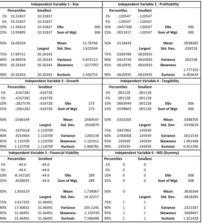
Below, we provide three tables regarding information concerning these variables, after already handling the outliers. Table 1 shows the summary statistics of the dependent variable, for both groups previously described in our study. Tables 2 and 3 show the detailed statistics for the independent variables, respectively, for the Financials and Non-Financials groups.

Table 1 – Descriptive Statistics (Dependent Variable)

Dependent Variable - Leverage (Financials) Dependent Variable - Leverage (Non-Financials)

Percentiles Smallest Percentiles Smallest

1% 0 0 1% .019499 .019499 5% 0 0 5% .019499 .019499 10% .0644524 0 Obs 305 10% .0521221 .019499 Obs 1835 25% .2301583 0 Sum of Wgt. 305 25% .1585335 .019499 Sum of Wgt. 1835 50% .3456197 Mean .3213423 50% .2963058 Mean .297643

Largest Std. Dev. .1570769 Largest Std. Dev. .1736537

75% .4298907 .5748129 75% .4151829 .6387459

90% .5219639 .5748129 Variance .0246732 90% .5523129 .6387459 Variance .0301556 95% .5748129 .5748129 Skewness -.4540208 95% .6387459 .6387459 Skewness .1937331 99% .5748129 .5748129 Kurtosis 2.484657 99% .6387459 .6387459 Kurtosis 2.225974

(22)

Table 2 – Descriptive Statistics (Independent Variables): Financials

Independent Variable 1 - Size Independent Variable 2 - Profitability

1% 10.31837 10.31837 1% -.120547 -.120547 5% 10.31837 10.31837 5% -.120547 -.120547 10% 11.93614 10.31837 Obs 306 10% -.0457306 -.120547 Obs 300 25% 13.93895 10.31837 Sum of Wgt. 306 25% .0011417 -.120547 Sum of Wgt. 300 50% 16.00334 Mean 15.78766 50% .0118434 Mean .0038285

Largest Std. Dev. 2.622044 Largest Std. Dev. .039218

75% 17.69721 20.26343 75% .0204789 .0610935 90% 18.89978 20.26343 Variance 6.875113 90% .0414739 .0610935 Variance .001538 95% 20.26343 20.26343 Skewness -.3277057 95% .0610935 .0610935 Skewness -1.777103 99% 20.26343 20.26343 Kurtosis 2.430753 99% .0610935 .0610935 Kurtosis 6.465634 Independent Variable 3 - Growth Independent Variable 4 - Tangibility

1% -.6167281 -.616728 1% .001128 .001128 5% -.6167281 -.616728 5% .001128 .001128 10% -.2827576 -.616728 Obs 273 10% .0063949 .001128 Obs 306 25% -.1061282 -.616728 Sum of Wgt. 273 25% .0199603 .001128 Sum of Wgt. 306 50% .0166149 Mean .0569547 50% .0310203 Mean .0388705

75% .1670518 1.110709 75% .0437962 .145939

90% .4253964 1.110709 Variance .1265139 90% .0783008 .145939 Variance .0011534 95% 1.110709 1.110709 Skewness 1.101911 95% .145939 .145939 Skewness 1.901468 99% 1.110709 1.110709 Kurtosis 5.460781 99% .145939 .145939 Kurtosis 6.451296

Independent Variable 5 - Financial Viability Independent Variable 6 - NID (Dummy)

1% -44.6 -44.6 1% 0 0 5% -44.6 -44.6 5% 0 0 10% -8.142105 -44.6 Obs 289 10% 0 0 Obs 308 25% .4438033 -44.6 Sum of Wgt. 289 25% 0 0 Sum of Wgt. 308 50% 1.850219 Mean 1.734067 50% 0 Mean .3636364

75% 3.617325 31.46491 75% 1 1

90% 17.40631 31.46491 Variance 205.1245 90% 1 1 Variance .2321587

95% 31.46491 31.46491 Skewness -1.159743 95% 1 1 Skewness .5669467

(23)

Table 3 – Descriptive Statistics (Independent Variables): Non-Financials

Independent Variable 1 - Size Independent Variable 2 - Profitability

1% 10.54737 10.54737 1% -.1423909 -.1423909 5% 10.54737 10.54737 5% -.1423909 -.1423909 10% 10.98661 10.54737 Obs 1835 10% -.0673193 -.1423909 Obs 1808 25% 11.92045 10.54737 Sum of Wgt. 1835 25% .0003432 -.1423909 Sum of Wgt. 1808 50% 12.993 Mean 13.331 50% .0397705 Mean .0313563

75% 14.59948 17.17213 75% .0748413 .149969 90% 16.07966 17.17213 Variance 3.442163 90% .116733 .149969 Variance .0049581 95% 17.17213 17.17213 Skewness .4540068 95% .149969 .149969 Skewness -.6729476 99% 17.17213 17.17213 Kurtosis 2.280017 99% .149969 .149969 Kurtosis 3.325458 Independent Variable 3 - Growth Independent Variable 4 - Tangibility

1% -.3871188 -.387118 1% .0123968 .0123968 5% -.3871188 -.387118 5% .0123968 .0123968 10% -.2141018 -.387118 Obs 1666 10% .0249062 .0123968 Obs 1835 25% -.0711818 -.387118 Sum of Wgt. 1666 25% .0856907 .0123968 Sum of Wgt. 1835 50% .0230367 Mean .0285161 50% .2040986 Mean .2544357

75% .1223136 .4489812 75% .3854673 .6953256

90% .288247 .4489812 Variance .0373108 90% .5638735 .6953256 Variance .0403969 95% .4489812 .4489812 Skewness .0603463 95% .6953256 .6953256 Skewness .7025498 99% .4489812 .4489812 Kurtosis 3.270309 99% .6953256 .6953256 Kurtosis 2.429915

Independent Variable 5 - Financial Viability Independent Variable 6 - NID (Dummy)

1% -12.46917 -12.4691 1% 0 0 5% -12.46917 -12.4691 5% 0 0 10% -5.163688 -12.4691 Obs 1807 10% 0 0 Obs 1859 25% .0006463 -12.4691 Sum of Wgt. 1807 25% 0 0 Sum of Wgt. 1859 50% 3.160747 Mean 6.679925 50% 0 Mean .3636364

75% 8.290769 50.16484 75% 1 1

90% 23.55924 50.16484 Variance 192.0168 90% 1 1 Variance .2315295

95% 50.16484 50.16484 Skewness 1.776922 95% 1 1 Skewness .5669467

99% 50.16484 50.16484 Kurtosis 6.178076 99% 1 1 Kurtosis 1.321429

As we can see from the tables above, we seem to have a relatively well-balanced panel of companies for the two groups. In terms of firm size, we can detect firms with low and high

(24)

size, without much difference in the means for both groups. When looking at Profitability, we also have included profitable and non-profitable firms for both groups, but it is interesting to see that the average Profitability for the Financials group is almost ten times the value for Non-Financial firms. When looking at Growth, we can see that we have included firms that are growing as well as firms that have decreasing revenues, which seem to be in a more mature state (some even in a state of bankruptcy). It also seems evident that we incorporate firms that have both high and low levels of Tangibility, and, as expected, the level of Tangibility is much higher for the Non-Financials group. As far as Financial Viability is concerned, we can see that even though we winsorized our variables at 5%, there is still a great level of variance.

In principle, since the data seems to be well-balanced, all this evidence combined should allow for a good overall representativeness of the results we obtained.

IV.2) Correlations

When looking at the correlations between the dependent variable and the explanatory variables incorporated in our model, conclusions can be drawn regarding the relationship of these variables with the level of Leverage. We can also check for high correlations between explanatory variables, that can evidence multicollinearity problems.

Tables 4 and 5, presented below, show Pearson’s correlation coefficients (which assumes a linear relationship between variables) for both groups in our analysis.

Table 4 – Pearson Coefficients (Financials group)

Pearson's Correlation Coefficients

Leverage Size Profitability Growth Tangibility Fin.Viability NID

Leverage 1.0000 Size 0.5542 1.0000 Profitability 0.1918 0.4238 1.0000 Growth -0.0322 -0.0113 0.1832 1.0000 Tangibility 0.0243 -0.2602 -0.4390 -0.0634 1.0000 Fin.Viability 0.0841 0.1969 0.7169 0.1972 -0.3045 1.0000 NID -0.0045 0.0464 -0.1363 -0.0249 -0.0775 -0.1088 1.0000

When looking at the correlation coefficients for the Financials group, one can see that the apparent existing high correlations all come from the variables Size and Profitability. Size

(25)

is the only variable that shows significant correlation with the dependent variable (around 50%), while Profitability shows significant correlation with other explanatory variables (namely Size, Tangibility and Financial Viability).

Another interesting aspect that we can observe from this Table is that for this group our variable of interest (NID) seems to be negatively correlated to our dependent variable (Leverage) and to the majority of the explanatory variables, except for Size. This could perhaps be an indicator, for future analyses, that Financial firms might verify an increase in Size, when in the presence of the NID (please note that correlation does not imply causality. It is simply an indicator of a possible positive relationship).

Table 5 – Pearson Coefficients (Non-Financials group)

Pearson's Correlation Coefficients

Leverage Size Profitability Growth Tangibility Fin.Viability NID

Leverage 1.0000 Size 0.0356 1.0000 Profitability -0.3012 0.2561 1.0000 Growth -0.1219 0.0713 0.3119 1.0000 Tangibility 0.2558 0.1057 -0.0361 -0.0189 1.0000 Fin.Viability -0.4936 0.0353 0.6598 0.1822 -0.1336 1.0000 NID 0.0573 0.0119 -0.1256 -0.1511 -0.0294 -0.0677 1.0000

Focusing on the Pearson coefficients for correlations in respect to the Non-Financials group, we can see some major differences when comparing to the Financials group: first of all, the variable that seems to have more correlation with the other in the Financials group (Size) is no longer highly correlated neither with our dependent variable, neither with Tangibility. It seems that the only relatively high correlation it maintained is with the variable Profitability. When considering this different group in our sample (Non-Financials), Profitability is still highly correlated with other explanatory variables, but in this case, mostly with Growth and Financial Viability. Another important difference, that goes against our initial intuition is that the NID is slightly positively correlated to Leverage. We will address this issue in the next sub-section.

IV.3) Regression Results

IV.3.1) Fixed vs Random-effects

(26)

use a Fixed-effects or a Random-effects regression for each of these groups. This decision was made based on the results of the Hausman test. Under this test, the null hypothesis is that a Random-effects regression is best suited for the data we are using, while the alternative hypothesis is that a Fixed-effects regression is better. We performed the Hausman test for the two groups in our study, and we evidenced that both for the Financials, and the Non-Financials groups, we would reject the null hypothesis and conclude that the Fixed-effects regression was best suited.

Below, we can see Tables 6 and 7 that show the results of the Hausman test, respectively for the Financial and Non-Financials group.

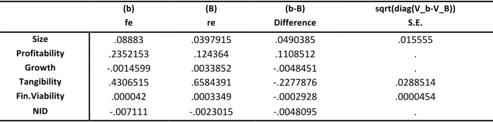
Table 6 – Hausman test results (Financials group)

(b) (B) (b-B) sqrt(diag(V_b-V_B))

fe re Difference S.E.

Size .08883 .0397915 .0490385 .015555 Profitability .2352153 .124364 .1108512 . Growth -.0014599 .0033852 -.0048451 . Tangibility .4306515 .6584391 -.2277876 .0288514 Fin.Viability .000042 .0003349 -.0002928 .0000454 NID _-.007111 _-.0023015 _-.0048095 _. Test: Ho: difference in coefficients not systematic chi2(6) = (b-B)'[(V_b-V_B)^(-1)](b-B) = 15.09 Prob>chi2 = 0.0196 (V_b-V_B is not positive definite)

As we can see, for a significance level of 5%, and with a Probabilitity>chi2 equal to 1.96%, we have to reject the null hypothesis that a Random-effects model is more appropriate, and therefore, the suited regression for the Financials group is, the Fixed-effects one. Table 7 will show the same results for the Non-Financials group.

(27)

Table 7 – Hausman test results (Non-Financials group)

(b) (B) (b-B) sqrt(diag(V_b-V_B))

fe re Difference S.E.

Size .0421669 .0169075 .0252594 .0057236 Profitability -.4395955 -.3937209 -.0458746 .0023662 Growth -.0019152 .0017696 -.0036848 . Tangibility .073604 .0904754 -.0168714 .007927 Fin.Viability -.0008 -.0014923 .0006924 .0000668 NID .0077866 .0075165 .0002701 . Test: Ho: difference in coefficients not systematic chi2(6) = (b-B)'[(V_b-V_B)^(-1)](b-B) = 69.26 Prob>chi2 = 0.0000 (V_b-V_B is not positive definite)

When looking at the Non-Financials group, it seems that for a significance level of 5%, we also have to reject the null hypothesis, and as a consequence, the Fixed-effects regression is, again, the most appropriate one.

Therefore, the regression outputs in the next sub-section were generated having these results into consideration.

IV.3.2) Regression Outputs

When looking at the first results obtained, they seem to be quite different for the two groups in our analysis. Below, in tables 8 and 9, we have the STATA outputs of the initial regressions we ran for both groups.

Table 8 - Initial Regression Output (Financials)

Fixed-effects (within) regression Number of obs = 257

Group variable: CompanyCode Number of groups = 28

R-sq: within = 0.1729 Obs per group: min = 5 between = 0.3667 avg = 9.2 overall = 0.3310 max = 10 F(6,223) = 7.77 corr(u_i, Xb) = -0.8178 Prob > F = 0.0000

(28)

Leverage Coef. Std. Err. z P>z [95% Conf. Interval] Size .08883 .0167697 5.30 0.000 .0557827 .1218773 Profitability .2352153 .2465845 0.95 0.341 -.2507187 .7211492 Growth -.0014599 .0147607 -0.10 0.921 -.0305483 .0276285 Tangibility .4306515 .2061464 2.09 0.038 .0244073 .8368957 Fin.Viability .000042 .000596 0.07 0.944 -.0011326 .0012166 NID -.007111 .0107481 -0.66 0.509 -.0282919 .0140699 _cons -1.104122 .264036 -4.18 0.000 -1.624447 -.583797

Looking at Table 8, we can see from the initial results regarding the financials group, that there are several relevant aspects to evidence: (i) Regarding the control variables, and as expected, the coefficients associated with the variables Size and Tangibility are positive. This goes in line with previous literature mentioned in Section 3. We also verify that the coefficients associated with the variables Growth, Profitability and Financial Viability are not significant, which makes it impossible for us to draw any conclusions since we cannot infer that they are statistically different from zero. This may derive from the small sample of firms that we have in the Financials group. (ii) In respect to the variable of interest, NID, we can also state that the associated coefficient associated to this variable is not statistically different from zero. Even if this coefficient is negative in the first column of Table 8, we can see from the 95% confidence interval in the last two columns that it belongs to a range that includes both positive and negative values. Therefore, based on Table 8, we can make no conclusions regarding the impact of the NID in the leverage ratio of Financial firms. (iii) finally, even though the R squared of the model is not high (around 33%), we can see that overall significance of the model is attested for a 5% significance level, since the Probability > F = 0.0000.

In the next sub-section (Regression Adaptations) we will perform some adjustments to this initial regression, to check if we can improve our results, since it seems that we have some variables with extremely high P values, which can be dropped from our initial regression.

(29)

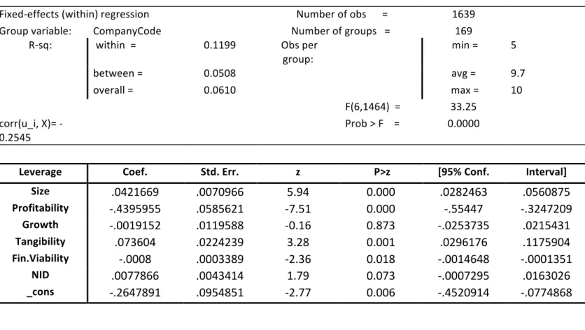
Table 9 - Initial Regression Output (Non-Financials)

R-sq: within = 0.1199 Obs per group: min = 5 between = 0.0508 avg = 9.7 overall = 0.0610 max = 10 F(6,1464) = 33.25 corr(u_i, X)= -0.2545 Prob > F = 0.0000

Leverage Coef. Std. Err. z P>z [95% Conf. Interval]

Size .0421669 .0070966 5.94 0.000 .0282463 .0560875 Profitability -.4395955 .0585621 -7.51 0.000 -.55447 -.3247209 Growth -.0019152 .0119588 -0.16 0.873 -.0253735 .0215431 Tangibility .073604 .0224239 3.28 0.001 .0296176 .1175904 Fin.Viability -.0008 .0003389 -2.36 0.018 -.0014648 -.0001351 NID .0077866 .0043414 1.79 0.073 -.0007295 .0163026 _cons -.2647891 .0954851 -2.77 0.006 -.4520914 -.0774868

When we look at Table 9, there are some immediate differences one can detect when comparing with the results from the Financials group. (i) It seems that for the Non-Financials group, the coefficient associated with Profitability is negative, which goes in line to what we expected. Also, the coefficient associated with Financial Viability changed, and is now negative, which again seems to go in line with existing literature and consequently, to what we expected beforehand. (ii) the coefficients associated with Size and Tangibility and did not change, and remain in line to what we were initially hoping to get. However, the coefficient associated to the variable Growth is not statistically different from zero, just like in Table 8. (iii) The coefficient associated with the variable of interest, NID, is positive, which is something that contradicts its intended effect and that we were not expecting to obtain. However, this is only true for a significance level of 10%. (iv) Finally, when considering a 5% significance level, all variables in the model seem to be significant, apart from Growth and our variable of interest – NID –. However, our variable of interest is significant when considering a 10% significance level, whereas Growth would imply a significance level above 80% to be significant. Again, in the next sub-section (Regression Adaptions) we will address these issues.

(30)

(around 8%), but the general significance of the model is attested by looking at the Probability > F which is 0.0000.

IV.3.3) Regression Adaptations

IV.3.3.1) Adaptations: Non-Financials group

After analysing the outputs from the initial regressions, the major issue we found was the positive coefficient associated with the NID variable, for the Non-Financials group. This would mean that, in the presence of the NID, firms would become more leveraged, which for us did not make sense given the theoretical framework we discussed before. Therefore, we decided to run regressions containing interaction terms of the control variables, multiplied by the variable of interest. In these regressions, we decided not to drop the variable Growth, since by doing so, we would not be able to assess whether the source of our changes in results would come from adding the interaction term, or from dropping the variable. Since the variable Growth was not significant, we decided not run any regressions including an interaction term with that variable. The different regressions we ran, for the Non-Financials group, are the following:

(i)Levi =β0 + β1Sizei + β2Profit.i + β3Growthi + β4Tang.i + β5FinViab.i + β6NID + β7Size*NID + Ɛi

(ii)Levi =β0 + β1Sizei + β2Profit.i + β3Growthi + β4Tang.i + β5FinViab.i + β6NID + β7Profit.*NID + Ɛi

(iii)Levi =β0 + β1Sizei + β2Profit.i + β3Growthi + β4Tang.i + β5FinViab.i + β6NID + β7Tang.*NID + Ɛi

(iv)Levi =β0 + β1Sizei + β2Profit.i + β3Growthi + β4Tang.i + β5FinViab.i + β6NID + β7FinViab.*NID + Ɛi

What we intended with these regressions was to check if we could identify at least one interaction variable with a negative coefficient associated, meaning that the NID would only

(31)

lead lower leverage ratios for firms with specific characteristics. Since the coefficient associated with the NID variable for the Financials group was already negative, there was no need to run these regressions for that particular group.

In our analysis, we will not show the outputs of regressions (iii) and (iv) since the coefficients associated with the interaction variable in all those regressions were still positive, and therefore, there seemed to be no need in evidencing them. However, Tables 10 and 11, presented below, show the output of regressions (i) and (ii), which seemed to provide interesting results, that go in line with the intended effect of the NID introduction (especially regression ii).

Table 10 - Adapted Regression (i) (Non-Financials)

R-sq: within = 0.1253 Obs per group: min = 5

between = 0.0467 avg = 9.7

overall = 0.0578 max = 10

F(7,1463) = 29.94

corr(u_i, X) = -0.2824 Prob > F = 0.0000

Size _.0470935 _.0072654 _6.48 _0.000 _.0328418 _.0613452 Profitability -.4462395 .0584448 -7.64 0.000 -.5608841 -.331595 Growth -.003227 .0119343 -0.27 0.787 -.0266372 .0201832 Tangibility _.0718734 _.0223704 _3.21 _0.001 _.027992 _.1157548 Fin.Viability -.000778 .0003381 -2.30 0.022 -.0014413 -.0001148 NID .09988 .0310063 3.22 0.001 .0390584 .1607017 sizeNID _-.0068945 _.0022985 _-3.00 _0.003 _-.0114032 _-.0023857 _cons -.3300289 .0976777 -3.38 0.001 -.5216323 -.1384256

For this regression, where we include an interaction variable equal to Size*NID (referred to as sizeNID in Table 10) we can see that even though the coefficients associated with the variables Size and NID by themselves are positive, the result of the interaction term between these two variables has a negative coefficient associated to it (with a P value of 0.000, which makes it significant). This means that the observed impact of the NID (for Non-Financial firms) in increasing Italian firms’ leverage ratios is smaller for larger firms. In that case, for larger size firms, the NID would lead to an increase in leverage ratios that is lower

(32)

than for smaller size firms. We can also see that the P value for the NID variable decreased to 0.001, and that the majority of the P values observed for the control variables makes them significant for a 5% significance level.

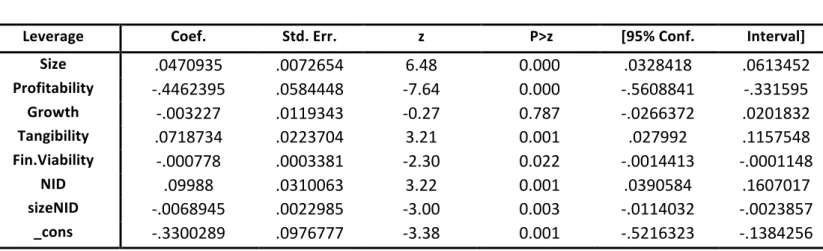
Table 11 - Adapted Regression (ii) (Non-Financials)

between = 0.0307 avg = 9.7

F(7,1463) = 32.78

corr(u_i, X) = -0.4062 Prob > F = 0.0000

Size .0546544 .0074421 7.34 0.000 .040056 .0692528 Profitability -.3177284 .0627009 -5.07 0.000 -.4407215 -.1947352 Growth -.0057848 .0118799 -0.49 0.626 -.0290882 .0175186 Tangibility .0690194 .022249 3.10 0.002 .025376 .1126627 Fin.Viability -.0007925 .000336 -2.36 0.018 -.0014517 -.0001333 NID .0166597 .0046365 3.59 0.000 .0075648 .0257546 profitNID -.3503235 .0680613 -5.15 0.000 -.4838316 -.2168154 _cons -.4347139 .1002558 -4.34 0.000 -.6313744 -.2380534

As far as Non-Financials are concerned, this seems to be our best regression in terms of results: not only are all coefficients associated with our variables significant (except for Growth), but we can see that, even though the NID seems to lead to an increase close to 2% in leverage ratios, for more profitable firms there is a high decrease in that effect (evidenced by the coefficient associated with our interaction term equal to around 35%). This is indeed more in line to what we initially hoped to achieve. We will later interpret this result in section IV.

From this point on, we will consider our Adapted Regression (ii) (for the Non-Financials group) as our Final Regression for this group, since it seems to be the most relevant.

IV.3.3.2) Adaptations: Financials group

The second set of adaptations to our initial regressions was done to the Financials group. Even though we had decided to avoid as much as possible to remove any variables

(33)

from our initial regressions, it seemed that due to the extremely high P value observed regarding the variables Growth and Financial Viability, we decided we had to run a regression where we would exclude these variables. There were other variables that had coefficients with relatively high P values, but we decided to keep them for the theoretical reasons mentioned above and due to the fact that, despite not significant at a 5%-10% level, their inclusion contributed to the overall significance for the model. The adapted regression ran was, therefore, the following:

(i) _{Levi =β0 + β1Sizei + β2Profit.i + β3Tang. i + β4NID + Ɛi}

Below, in Table 12, we can see the results of that regression, which was mainly intended at increasing the significance of the negative coefficient associated with the NID variable (meaning: decreasing its P value).

Table 12 - Adapted Regression (i) (Financials)

between = 0.4040 avg = 10.7

F(4,267) = 12.18

corr(u_i, X) = -0.7400 Prob > F = 0.0000

Size .0779012 .0131714 5.91 0.000 .0519681 .1038342

Profitability .1920912 .1996191 0.96 0.337 -.2009366 .585119

Tangibility .464106 .1876835 2.47 0.014 .094578 .833634

NID -.011799 .0107536 -1.10 0.274 -.0329716 .0093736

_cons -.9218063 .205866 -4.48 0.000 -1.327133 -.516479

As evidenced from the results above, we can see that after excluding the variables Growth and Financial Viability from our model, the significance of the coefficient associated with our variable of interest also improved (P value decreased to around half of its value in the initial regression). Also, even though we cannot state that the coefficient associated to our variable of interest is significantly different from zero, we can observe that its P value decreased to almost half of its initial value.