Interest rates dynamics: Contribution of
macroeconomic information in four
European markets
I S A B E L M A L D O N A D O C A R L O S P I N H O F R A N C I S C O R O D R Í G U E Z D E P R A D O C A R L A A Z E V E D O L O B O X I I I I B E R I A N I N T E R N A T I O N A L B U S I N E S S C O N F E R E N C E 2 0 - 2 1 O C T O B E R 2 0 1 7 I S C T E - I N S T I T U T O U N I V E R S I T Á R I O D E L I S B O AInterest rates dynamics
Predictive ability in the term structure of interest rates dynamic models;
Using data from German, English, Spanish and Portuguese public debts, the inflation rate and the annual variation of the industrial production index;
Results obtained, for the period from January 1990 to December 2012, indicate that the consideration of macroeconomic factors has a positive contribution to the improvement of forecasts for different countries and maturities.
Interest rates dynamics
Dynamic ModelsVasicel (1977), Cox et. al (1985), Duffie and Kan (1996), Ang and Piazzesi (2003)
Statistic Models
McCulloch (1971, 1975), Nelson and Siegel (1987), Svensson (1994)
With of macroeconomic variables
Data and Methodology
Public debt interest rates of four European countries: Germany, United Kingdom, Spain and Portugal
Period: from January 1990 to December 2012
Monthly observations
Maturities of 3, 6, 9, 12, 24, 36, 48, 60, 72, 84, 96, 108 and 120 months
For unobserved maturities, we used the non-parametric interpolation procedure proposed by McCulloch (1971, 1975)
Macroeconomic variables: consumer price index (CPI) and industrial production index, total industry excluding construction (ICI).
Results
•
Adjustment quality•
Out-Off-Sample Predictive Ability•
Contribution of Macroeconomic VariablesResults - adjustment analysis
Estimation and adjustment quality:
•
Dynamic Nelson and Siegel model (DNS)•
Affine Dynamic Nelson and Siegel model (ADNS)•
Estimation for the period January 1990 to December 2012, assuming autoregressive specifications of first order, AR(1), and vector autoregressive specifications of first order, VAR(1).Results - adjustment analysis
Estimation of the DNS-AR(1)
Germany Lt-1 St-1 Ct-1 µ q λ LogL Lt 0.9912 - - 0.0507 0.0025 0.051 -14499.1 St 0 0.9134 - -0.0199 0.0022 Ct 0 0 0.8904 -0.0101 0.0023 United Kingdom Lt-1 St-1 Ct-1 µ q λ LogL Lt 0.9991 0 0 0.0627 0.0022 0.073 -14748.5 St 0 0.9868 0 -0.0197 0.0024 Ct 0 0 0.9803 -0.0126 0.0024 Portugal Lt-1 St-1 Ct-1 µ q λ LogL Lt 0.9988 0 0 0.0597 0.0023 0.06 -12417.1 St 0 0.943 0 -0.0213 0.0025 Ct 0 0 0.8923 -0.0124 0.003 Spain Lt-1 St-1 Ct-1 µ q λ LogL Lt 0.9872 0 0 0.0597 0.0023 0.065 -12825.6 St 0 0.9371 0 -0.0212 0.002 Ct 0 0 0.896 -0.0126 0.0028
Results - adjustment analysis
Estimation of the DNS-VAR(1)
Table 2 present the transition matrix A, the media vector µ and the q matrix.
Germany Lt-1 St-1 Ct-1 µ qL q_S q_C λ LogL Lt 0.9859 0.0048 0.0086 0.0951 0.0028 - - 0.052 -14492.1 St -0.0077 0.9279 0.0595 0.0444 0.0023 0.00203 -Ct 0.0415 0.0512 0.9265 0.3365 0.0026 0.00284 0.00271 United Kingdom Lt-1 St-1 Ct-1 µ qL q_S q_C λ LogL Lt 0.9997 0.0046 0.0015 0.0646 0.0021 - - 0.072 -14750.5 St 0.0005 0.969 0.0653 -0.0209 0.002 0.0023 -Ct -0.0067 -0.0864 0.9741 -0.0123 0.0021 0.0022 0.0024 Portugal Lt-1 St-1 Ct-1 µ qL q_S q_C λ LogL Lt 0.9973 0.0095 0.0094 0.0578 0.003 - - 0.0672 -12407.3 St 0.0094 0.9261 0.0102 -0.0223 0.0024 0.0018 -Ct 0.0104 0.0137 0.9033 -0.0057 0.0049 0.0029 0.0021 Spain Lt-1 St-1 Ct-1 µ qL q_S q_C λ LogL Lt 0.9862 0.0561 0.0116 0.0635 0.0022 - - 0.069 -12807.3 St 0.0025 0.9074 0.0495 -0.0275 0.0025 0.0027 -Ct 0.0873 -0.0459 0.8947 -0.018 0.0035 0.003 0.0028
Results - adjustment analysis
Estimation of the ADNS-AR(1)
Table 3 presents the estimated parameters for the Kp matrix, θ vector and diagonal diffusion matrix Σ for ADNS model.
Germany K KL KS KC θ Σ σL σS σC λ KL 0.1259 - - 0.061 σL 0.005 0 0 0.0681 KS - 0.2305 - -0.0185 σS 0 0.0062 0 KC - - 1.0623 -0.0115 σC 0 0 0.0059 United Kingdom K KL KS KC θ Σ σL σS σC λ KL 0.1152 - - 0.0881 σL 0.005 0 0 0.07 KS - 0.2726 - -0.0174 σS 0 0.0062 0 KC - - 1.1602 -0.0092 σC 0 0 0.0059 Portugal K KL KS KC θ Σ σL σS σC λ KL 0.0725 - - 0.0713 σL 0.0025 0 0 0.056 KS - 0.2605 - -0.0283 σS 0 0.01 0 KC - - 0.9964 -0.0031 σC 0 0 0.0038 Spain K KL KS KC θ Σ σL σS σC λ KL 0.1508 - - 0.066 σL 0.0031 0 0 0.0671 KS - 0.1386 - -0.0252 σS 0 0.0063 0 KC - - 0.876 -0.014 σC 0 0 0.0102
Results - adjustment analysis
Estimation of the ADNS-VAR(1)
Table 4 presents the estimated parameters for the Kp matrix, θ vector and diagonal diffusion matrix Σ for ADNS model.
Germany K KL KS KC θ Σ σL σS σC λ KL 0.02765 1.6931 -1.1819 0.0521 σL 0.0028 0.057 KS -0.491 0.6457 -0.6817 -0.0179 σS 0.002 0.0021 KC -0.7436 0.9196 1.2368 -0.0073 σC 0.0023 0.0025 0.0027 United Kingdom K KL KS KC θ Σ σL σS σC λ KL 0.1093 -0.2833 0.207 0.0625 σL 0.0018 0.083 KS -0.0103 0.2979 0.4087 -0.0398 σS 0.0022 0.002 KC 0.2557 0.0524 1.3231 -0.008 σC 0.0024 0.0027 0.003 Portugal K KL KS KC θ Σ σL σS σC λ KL 0.1933 -0.4819 0.1497 0.0972 σL 0 0.0565 KS 0.13 0.2383 -0.8557 0.0115 σS 0.0028 0.0028 KC 0.3553 1.9332 1.3287 -0.0064 σC 0.0026 0.0027 0.0038 Spain K KL KS KC θ Σ σL σS σC λ KL 0.1633 -0.2318 0.1097 0.0735 σL 0 0.067 KS 0.1408 0.2873 -0.7507 -0.0375 σS 0.0042 0.0025 KC 0.2378 1.0335 1.1743 -0.038 σC 0.0037 0.0032 0.0027
Results - adjustment analysis
Root mean squared error for Germany, United Kingdom, Portugal and Spain
Maturity Germany 3 6 9 12 24 36 48 60 72 84 96 108 120 DNS-AR(1) 0.2863 0.179 0.1277 0.1087 0.0784 0.0991 0.1187 0.1141 0.0905 0.057 0.0288 0.0504 0.0884 DNS-VAR(1) 0.0672 0.0812 0.1144 0.1287 0.0825 0.0255 0.0471 0.0534 0.0394 0.023 0.0451 0.0809 0.1215 ADNS-AR(1) 0.0908 0.0428 0.0755 0.0914 0.0641 0.0553 0.08000 0.0806 0.0613 0.0342 0.0367 0.0699 0.1086 ADNS-VAR(1) 0.0619 0.0535 0.0878 0.1037 0.0631 0.0321 0.0614 0.0653 0.0476 0.023 0.0369 0.0739 0.1152 United Kingdom 3 6 9 12 24 36 48 60 72 84 96 108 120 DNS-AR(1) 0.2578 0.1508 0.0929 0.0863 0.0749 0.0975 0.1491 0.1831 0.1906 0.1387 0.0686 0.1173 0.2201 DNS-VAR(1) 0.1200 0.0824 0.1200 0.1420 0.1109 0.0577 0.1073 0.1477 0.1604 0.1135 0.0648 0.1374 0.2388 ADNS-AR(1) 0.1597 0.0784 0.0987 0.1252 0.1044 0.0800 0.1276 0.1646 0.1746 0.1275 0.0766 0.1343 0.2335 ADNS-VAR(1) 0.1223 0.0957 0.133 0.1539 0.1222 0.0633 0.1067 0.1453 0.1571 0.1100 0.0674 0.1437 0.2448 Portugal 3 6 9 12 24 36 48 60 72 84 96 108 120 DNS-AR(1) 0.2247 0.1596 0.1302 0.111 0.1497 0.1753 0.2393 0.2819 0.2555 0.2772 0.1704 0.0964 0.2453 DNS-VAR(1) 0.2556 0.2036 0.1098 0.0890 0.2081 0.1411 0.1409 0.1689 0.1514 0.1837 0.1650 0.1983 0.3251 ADNS-AR(1) 0.1576 0.0350 0.0853 0.1174 0.1830 0.1195 0.1689 0.2045 0.1959 0.2282 0.1447 0.1288 0.3017 ADNS-VAR(1) 0.1296 0.0436 0.1221 0.1577 0.2021 0.1243 0.1735 0.2224 0.1919 0.2031 0.1739 0.2026 0.3650 Spain 3 6 9 12 24 36 48 60 72 84 96 108 120 DNS-AR(1) 0.3217 0.1985 0.1968 0.2154 0.2511 0.3442 0.4378 0.3623 0.2464 0.2084 0.1535 0.115 0.3567 DNS-VAR(1) 0.1388 0.0796 0.1423 0.1744 0.116 0.2507 0.385 0.3307 0.2465 0.2232 0.1659 0.1056 0.3379 ADNS-AR(1) 0.1385 0.0794 0.1424 0.1745 0.1159 0.2505 0.3848 0.3306 0.2465 0.2233 0.1659 0.1057 0.3379 ADNS-VAR(1) 0.1895 0.0796 0.1296 0.1716 0.1054 0.2119 0.3558 0.3128 0.2407 0.2214 0.1672 0.1103 0.3437
Table 5 shows the RMSE for the estimation of Diebold-Li models with autoregressive first-order process DNS-AR(1), with vector autoregressive first-order process, DNS-VAR(1), and also for the affine models ADNS-AR(1) and ADNS-VAR(1).
Results - adjustment analysis
The degree of adjustment between the observed rates and estimated rates is generally high for the different models.
The estimation results shows that none of the models analyzed seems to be clearly
superior to the others in terms of adjustment.
The adjustment analysis allows us to state that, as regards the temporal dimension, DNS and ADNS models, have a good adjustment in market stability phases, however, in periods of high volatility the adjustment quality decreases considerably.
Results – out off sample predictive ability
The data set was divided into two subsets:
an initial, January 1990 to December 2002 used for the initial estimation
and a second subset, January 2003 to December 2012, used for forecasting
Methodology based on the rolling windows method with 120 observations
Prediction horizons set: h = 1, 3, 6, 9, 12, 15 and 18 months
For the 13 maturities estimated (3, 6, 9, 12, 24, 36, 48, 60, 72, 84, 96, 108 and 120 months) was determined the RMSE as well as the ratio RMSE and RMSE of the random walk model (RW).
Results – out off sample predictive ability
Root mean squared error, Germany
Maturity A) RW 3 6 9 12 24 36 48 60 72 84 96 108 120 h=1 0.23 0.216 0.209 0.207 0.227 0.235 0.231 0.224 0.217 0.211 0.208 0.204 0.203 h=3 0.475 0.476 0.479 0.482 0.493 0.484 0.461 0.437 0.414 0.395 0.38 0.366 0.357 h=6 0.775 0.78 0.783 0.786 0.772 0.74 0.702 0.665 0.629 0.598 0.573 0.551 0.534 h=9 1.002 1.001 0.998 0.993 0.935 0.875 0.821 0.773 0.73 0.693 0.661 0.636 0.616 h=12 1.217 1.211 1.201 1.186 1.077 0.983 0.912 0.856 0.809 0.769 0.735 0.708 0.686 h=15 1.419 1.41 1.396 1.375 1.231 1.109 1.021 0.955 0.902 0.859 0.825 0.797 0.775 h=18 1.6 1.591 1.576 1.554 1.395 1.251 1.143 1.062 0.999 0.949 0.909 0.878 0.853 B) DNS-AR(1) 3 6 9 12 24 36 48 60 72 84 96 108 120 h=1 0.273 0.218 0.209 0.213 0.225 0.247 0.27 0.271 0.252 0.227 0.208 0.207 0.224 h=3 0.507 0.477 0.474 0.476 0.486 0.49 0.489 0.474 0.444 0.41 0.38 0.359 0.35 h=6 0.801 0.78 0.775 0.774 0.763 0.746 0.727 0.699 0.66 0.616 0.574 0.538 0.512 h=9 1.029 1 0.985 0.975 0.924 0.884 0.851 0.813 0.766 0.714 0.662 0.618 0.581 h=12 1.245 1.209 1.184 1.162 1.064 0.996 0.948 0.902 0.849 0.792 0.736 0.686 0.643 h=15 1.445 1.406 1.376 1.347 1.217 1.124 1.061 1.005 0.945 0.884 0.824 0.771 0.724 h=18 1.621 1.586 1.556 1.526 1.379 1.264 1.183 1.112 1.043 0.974 0.907 0.848 0.797 C) DNS-VAR(1) 3 6 9 12 24 36 48 60 72 84 96 108 120 h=1 0.25 0.215 0.219 0.226 0.231 0.242 0.261 0.262 0.245 0.222 0.207 0.208 0.228 h=3 0.495 0.477 0.479 0.484 0.491 0.489 0.485 0.468 0.439 0.407 0.377 0.358 0.351 h=6 0.794 0.78 0.78 0.781 0.767 0.746 0.724 0.695 0.655 0.612 0.57 0.536 0.51 h=9 1.018 0.996 0.985 0.976 0.925 0.882 0.847 0.808 0.76 0.709 0.658 0.614 0.577 h=12 1.232 1.201 1.18 1.161 1.064 0.993 0.943 0.896 0.843 0.786 0.73 0.681 0.638 h=15 1.433 1.399 1.372 1.346 1.217 1.121 1.056 0.999 0.939 0.878 0.818 0.765 0.718 h=18 1.613 1.582 1.556 1.528 1.382 1.264 1.179 1.107 1.037 0.968 0.901 0.842 0.79
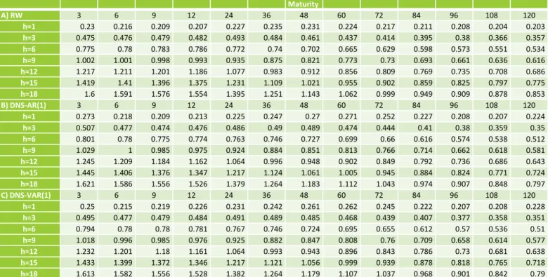
Table 6 presents in three panels the RMSE for Germany, for out-of-sample forecasts of RW model (Panel A), Latent Factor Model DNS-AR(1) (Panel B) and Latent Factor Model DNS-VAR(1) (Panel C). In all cases, the forecasts were made for the period between 01: 2003 and 12:2012. The forecasts were made for the maturities of 3, 6, 9, 12, 24, 36, 48, 60, 72, 84, 96, 108 and 120 months, and
Results – out off sample predictive ability
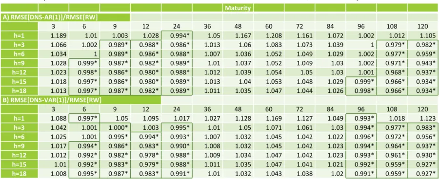
Root mean squared error ratio for DNS-AR and DNS-VAR models, Germany
Table 7 presents in two panels the RMSE ratio for Germany, for out-of-sample forecasts, for the autoregressive of first order process AR (1) in latent factors model (DNS) (Panel A) and for the vector autoregressive of first order process VAR (1) in latent factors model (DNS) (Panel B). The values marked with the symbol * correspond to the forecast horizons (h) and maturities for which the models show a superior performance. The forecasts in all cases presented were made for the period between 01:2003 and 12:2012. The forecasts were made for the maturities of 3, 6, 9, 12, 24, 36, 48, 60, 72, 84, 96, 108 and 120 months and for forecast horizons of 1 to 18 months (h=1, h=3, h=6, h=9, h=12, h=15 and h=18).
Maturity A) RMSE[DNS-AR(1)]/RMSE[RW] 3 6 9 12 24 36 48 60 72 84 96 108 120 h=1 1.189 1.01 1.003 1.028 0.994* 1.05 1.167 1.208 1.161 1.072 1.002 1.012 1.105 h=3 1.066 1.002 0.989* 0.988* 0.986* 1.013 1.06 1.083 1.073 1.039 1 0.979* 0.982* h=6 1.034 1 0.989* 0.986* 0.988* 1.007 1.036 1.052 1.049 1.029 1.002 0.977* 0.959* h=9 1.028 0.999* 0.987* 0.982* 0.989* 1.01 1.037 1.052 1.049 1.03 1.002 0.971* 0.943* h=12 1.023 0.998* 0.986* 0.980* 0.988* 1.012 1.039 1.054 1.05 1.03 1.001 0.968* 0.937* h=15 1.018 0.997* 0.986* 0.980* 0.989* 1.013 1.04 1.053 1.048 1.029 0.999* 0.966* 0.934* h=18 1.013 0.997* 0.987* 0.982* 0.989* 1.011 1.035 1.047 1.044 1.026 0.998* 0.966* 0.934* B) RMSE[DNS-VAR(1)]/RMSE[RW] 3 6 9 12 24 36 48 60 72 84 96 108 120 h=1 1.088 0.997* 1.05 1.095 1.017 1.027 1.128 1.169 1.127 1.049 0.993* 1.018 1.123 h=3 1.042 1.001 1.000* 1.003 0.995* 1.01 1.05 1.071 1.061 1.03 0.994* 0.977* 0.983* h=6 1.025 1.001 0.995* 0.994* 0.993* 1.007 1.032 1.045 1.042 1.022 0.996* 0.972* 0.956* h=9 1.017 0.994* 0.986* 0.983* 0.990* 1.008 1.032 1.045 1.042 1.023 0.994* 0.964* 0.937* h=12 1.012 0.992* 0.982* 0.978* 0.988* 1.009 1.034 1.047 1.042 1.023 0.993* 0.961* 0.930* h=15 1.01 0.992* 0.983* 0.979* 0.988* 1.011 1.035 1.047 1.041 1.021 0.992* 0.959* 0.927* h=18 1.008 0.995* 0.987* 0.983* 0.991* 1.01 1.032 1.043 1.038 1.02 0.991* 0.959* 0.927*
Results – out off sample predictive ability
In general, the results obtained for the forecasts out of sample, indicate a superiority of the and VAR (1) models relative to the AR (1) model.
The VAR model (1) performs well in terms of forecasting, however, is not systematically superior to RW model in all maturities.
In our case, grouping the performance indicators for short-term maturities (3 to 12 months), medium term (24 to 60 months) and long term (72 to 120 months) we note that as the
Results – contribution of macroeconomic
variables
In order to assess the impact of the introduction of macroeconomic variables in the dynamic models, we added to the state vector of the first order VAR(1) model two macroeconomic variables, representing:
inflation rate
Results – contribution of macroeconomic
variables
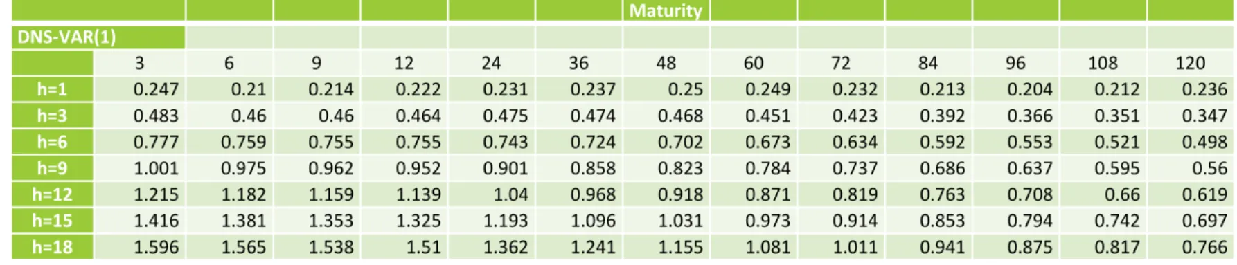
Root mean squared error of DNS-VAR models with Macroeconomic Factors, Germany
Maturity DNS-VAR(1) 3 6 9 12 24 36 48 60 72 84 96 108 120 h=1 0.247 0.21 0.214 0.222 0.231 0.237 0.25 0.249 0.232 0.213 0.204 0.212 0.236 h=3 0.483 0.46 0.46 0.464 0.475 0.474 0.468 0.451 0.423 0.392 0.366 0.351 0.347 h=6 0.777 0.759 0.755 0.755 0.743 0.724 0.702 0.673 0.634 0.592 0.553 0.521 0.498 h=9 1.001 0.975 0.962 0.952 0.901 0.858 0.823 0.784 0.737 0.686 0.637 0.595 0.56 h=12 1.215 1.182 1.159 1.139 1.04 0.968 0.918 0.871 0.819 0.763 0.708 0.66 0.619 h=15 1.416 1.381 1.353 1.325 1.193 1.096 1.031 0.973 0.914 0.853 0.794 0.742 0.697 h=18 1.596 1.565 1.538 1.51 1.362 1.241 1.155 1.081 1.011 0.941 0.875 0.817 0.766
Table 8 presents the RMSE for Germany, for the out-of-sample forecasts of the vector autoregressive of first order process VAR (1) for the latent factors model (DNS) with macroeconomic variables. In all cases presented the forecasts were carried out for the period from 1:2003 to 12:2012. The forecasts were made for the maturities of 3, 6, 9, 12, 24, 36, 48, 60, 72, 84, 96 108 and 120 months, and for forecast horizons of 1 to 18 months (h=1, h=3, h=6, h=9, h=12, h=15 and h=18).
Results – contribution of macroeconomic
variables
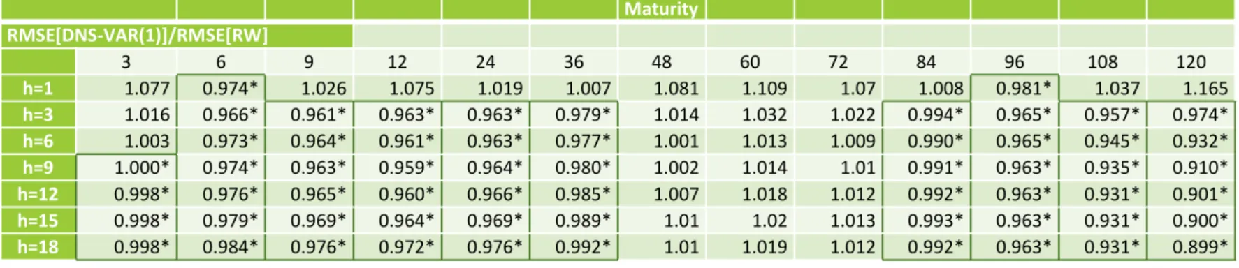
Root mean squared error ratio of the DNS-VAR model with Macroeconomic Factors, Germany
Table 9 shows the RMSE ratio for Germany, for the out-of-sample predictions of the vector autoregressive first order VAR (1) for latent factors model (DNS) and macroeconomic variables. The values marked with the symbol * correspond to the forecast horizons (h) and maturities for which the models perform better. The predictions in all cases were carried out for the period from 1:2003 to 12:2012. The forecasts were made for the maturities of 3, 6, 9, 12, 24, 36, 48, 60, 72, 84, 96, 108 and 120 months, and for forecast horizons of 1 to 18 months (h=1, h=3, h=6, h=9, h=12, h=15 and h=18).
Maturity RMSE[DNS-VAR(1)]/RMSE[RW] 3 6 9 12 24 36 48 60 72 84 96 108 120 h=1 1.077 0.974* 1.026 1.075 1.019 1.007 1.081 1.109 1.07 1.008 0.981* 1.037 1.165 h=3 1.016 0.966* 0.961* 0.963* 0.963* 0.979* 1.014 1.032 1.022 0.994* 0.965* 0.957* 0.974* h=6 1.003 0.973* 0.964* 0.961* 0.963* 0.977* 1.001 1.013 1.009 0.990* 0.965* 0.945* 0.932* h=9 1.000* 0.974* 0.963* 0.959* 0.964* 0.980* 1.002 1.014 1.01 0.991* 0.963* 0.935* 0.910* h=12 0.998* 0.976* 0.965* 0.960* 0.966* 0.985* 1.007 1.018 1.012 0.992* 0.963* 0.931* 0.901* h=15 0.998* 0.979* 0.969* 0.964* 0.969* 0.989* 1.01 1.02 1.013 0.993* 0.963* 0.931* 0.900* h=18 0.998* 0.984* 0.976* 0.972* 0.976* 0.992* 1.01 1.019 1.012 0.992* 0.963* 0.931* 0.899*
Results – contribution of macroeconomic
variables
The results obtained point to an improvement in the forecast ability for the dynamic Nelson and Siegel model after the incorporation of macroeconomic variables.
As can be seen by the RMSE for most of the maturities and forecast horizons,
macroeconomic information contributes positively to the predictive ability of the model, in the case of Germany (Table 8), UK, Spain and Portugal.
The positive contribution of the inclusion of macroeconomic data is also reflected in an
Results – contribution of macroeconomic
variables
Even if, in many cases, the RW model continue to provide a superior foresight, the model VAR(1) considering the two mentioned macroeconomic factors, performs better for short maturities in the United Kingdom, and short maturities as well as for long maturities in the case of Germany, Spain and Portugal.
These results reinforce the current assumption in literature that the incorporation of macroeconomic information has a clear contribution to the improvement of forecasting ability.
Results – temporal evolution of errors
analysis
In order to analyze the evolution of the model's performance compared to models that do not include macroeconomic data, we study the evolution of the RMSE for the latent factors models (DNS) compared to the RMSE of the random walk model for the autoregressive of first order process AR(1)), the vector autoregressive of first order process
(DNS-VAR(1)) and the autoregressive of first order process, incorporating macroeconomic factors (DNS-VAR(1)MF).
The data are for the period from January 2003 to December 2012, and for maturities of 1, 5 and 10 years and forecasting horizons 3 and 6 months.
Results – temporal evolution of errors
analysis
Results – temporal evolution of errors
analysis
Results – temporal evolution of errors
analysis
Results – temporal evolution of errors
analysis
Results – temporal evolution of errors
analysis
As we have seen by examining the Figures 2 to 5, for maturities of 1, 5 and 10 years and prediction horizons of 3 and 6 months, the performance of AR(1), VAR(1) and VAR(1)MF models varies over January 2003 to December 2012.
The analysis of the evolution of RMSE series allows us to conclude that, in general, the
inclusion of macroeconomic data in dynamic models, namely information on the inflation rate and the annual change in the industrial production index, improves its relative performance, which can be seen through the evolution of the RMSE series of the model with best
Conclusion
We find that, for the countries under study, for the period considered and for the dynamic specification of these factors, there is a superiority of the results obtained for the RW and VAR(1) models when compared whit the AR(1) model. The VAR(l) model performs well in terms of prediction, however this is not systematically higher than the RW model in all maturities.
The inclusion of macroeconomic variables representative of inflation and the annual growth of industrial production index shows a positive contribution to the forecasts improvement, for the 4 countries analyzed, for all maturities and for all forecast horizons.
Even if, in many cases, the RW model continue to provide a superior foresight, the model VAR(l) considering these two macroeconomic factors, performs better for short maturities in the United Kingdom and for short maturities and long maturities in the case of Germany, Spain and Portugal.