Behavioral modeling optimization and enhancement for high-speed analog mixed-signal I/O interfaces

WAEL DGHAIS

Otimização

e

Melhoria

da

Modulação

Comportamental para os Interfaces de E/S

Analógica e de Sinal Misto de Alta Velocidade

Behavioral

Modeling

Optimization

and

Enhancement for High-Speed Analog Mixed-Signal

I/O interfaces

DSP / LOGIC CORE

Digital Domain

V

DD

Chip #1

V

DD

Chip #2

Output

Interface

Input

Interface

DSP / LOGIC CORE

Digital Domain

v

2(t)

i

2(t)

v

1(t)

Analog Domain

Modelling

Transmission Medium

Wael Dghais

Behavioral Modeling Optimization and Enhancement

for High-Speed Analog Mixed-Signal I/O interfaces

Tese apresentada à Universidade de Aveiro para cumprimento dos requisitos necessários à obtenção do grau de Doutor em Engenharia Electrotécnica, realizada sob a orientação científica do Doutor José Carlos Pedro, Professor Catedrático, e co-orientação científica do Doutor Telmo Reis Cunha, Professor Auxiliar, do Departamento de Electrónica, Telecomunicações e Informática da Universidade de Aveiro.

Apoio financeiro da FCT no âmbito do QREN-POPH na Tipologia 4.1 – Formação Avançada, comparticipado pelo Fundo Social Europeu e por fundos nacionais do MEC com a referência SFRH / BD / 63927 / 2009.

O júri

Presidente Prof. Doutor Paulo Jorge de Melo Matias Faria de Vila Real

Professor Catedrático do Departamento de Engenharia Civil da Universidade de Aveiro.

Prof. Doutor Luís Miguel Teixeira d' Ávila Pinto da Silveira

Professor Catedrático do Instituto Superior Técnico, Universidade de Lisboa.

Prof. Doutor Vítor Manuel Grade Tavares,

Professor Auxiliar da Faculdade de Engenharia da Universidade do Porto.

Prof. Doutor Luís Filipe Mesquita Nero Moreira Alves,

Professor Auxiliar do Departamento de Electrónica, Telecomunicações e Informática da Universidade de Aveiro.

Prof. Doutor. José Carlos Esteves Duarte Pedro,

Professor Catedrático do Departamento de Electrónica, Telecomunicações e Informática da Universidade de Aveiro (Orientador).

 AGRADECIMENTOS I have been especially lucky to have so many great people helping me out with different aspects of my life and work in Aveiro, Portugal, at the Instituto de Telecomunicações (IT) and the Universidade de Aveiro.

I would like to express my sincere gratitude to my supervisor, Professor José Carlos Pedro, for his guidance and support during my graduate studies. I will always be grateful for his generous supports, insightful suggestions and encouragement during the PhD course and the research work. José takes every aspect of his advising role seriously by analyzing ideas and finding their faults. Moreover, I always find him concerned and available for help. José is also a great teacher who trains his students to break down problems to simple fundamental concepts.

My co-supervisor, Professor Telmo Reis Cunha, was always available for any questions and discussions. I have also benefited from taking his courses in nonlinear system identification theory. His approach to teaching and explaining the difficulties by illustrative examples is very practical. A good part of my PhD work relies on what I have learned from his course and the results of many fruitful discussions.

I would like to thank professors Luis Nero Neves and Fethi Bellamin for their orientations in the beginning of my research and their recommendation’s letters to get the Portuguese scholarship from FCT (Fundação para a Ciência e a Tecnologia).

I would like also to express my gratitude for my colleague Hugo Miguel Teixeira for many hours of fascinating discussions, strong intuition, and collaborative research work. I am grateful also to the rest of our wireless group at IT who helped me by providing valuable feedback within their areas of expertise.

I would especially like to thank my wife, Malek Souilem, for her supports, discussions and sacrifices. It certainly wouldn’t have been possible for me to get this far without the sacrifices of my parents, Habib Dghais and Rafika Kalboussi, my grand-mother Khadija Souilem, and my brothers Mohamed Ashraf Dghais and Ghassen Dghais. This dissertation is a result of their 29 years of infinite love and support, and for that, they own all my success. This dissertation is dedicated to them as a token of thankfulness and gratitude.

Finally, my thanks go to the president of the PhD committee and the examiner for honoring me with their presence and taking the time to evaluate my work.

Palavras-chave Interfaces analógicas e mistas de entrada/saída do circuito integrado, identificação de sistemas não-lineares, Integridade de sinal, aproximação da função, modelação comportamental baseados na tabela, análise transiente, extracção de modelo no domínio do tempo e no domínio da frequência.

 Resumo A integridade do sinal em sistemas digitais interligados de alta velocidade, e avaliada através da simulação de modelos físicos (de nível de transístor) é custosa de ponto vista computacional (por exemplo, em tempo de execução de CPU e armazenamento de memória), e exige a disponibilização de detalhes físicos da estrutura interna do dispositivo.

Esse cenário aumenta o interesse pela alternativa de modelação comportamental que descreve as características de operação do equipamento a partir da observação dos sinais eléctrico de entrada/saída (E/S).

Os interfaces de E/S em chips de memória, que mais contribuem em carga computacional, desempenham funções complexas e incluem, por isso, um elevado número de pinos. Particularmente, os buffers de saída são obrigados a distorcer os sinais devido à sua dinâmica e não linearidade. Portanto, constituem o ponto crítico nos de circuitos integrados (CI) para a garantia da transmissão confiável em comunicações digitais de alta velocidade.

Neste trabalho de doutoramento, os efeitos dinâmicos não-lineares anteriormente negligenciados do buffer de saída são estudados e modulados de forma eficiente para reduzir a complexidade da modelação do tipo caixa-negra paramétrica, melhorando assim o modelo standard IBIS. Isto é conseguido seguindo a abordagem semi-física que combina as características de formulação do modelo caixa-negra, a análise dos sinais eléctricos observados na E/S e propriedades na estrutura física do

buffer em condições de operação práticas.

Esta abordagem leva a um processo de construção do modelo comportamental fisicamente inspirado que supera os problemas das abordagens anteriores, optimizando os recursos utilizados em diferentes etapas de geração do modelo (ou seja, caracterização, formulação, extracção e implementação) para simular o comportamento dinâmico não-linear do buffer. Em consequência, contributo mais significativo desta tese é o desenvolvimento de um novo modelo comportamental analógico de duas portas adequado à simulação em overclocking que reveste de um particular interesse nas mais recentes usos de interfaces de E/S para memória de elevadas taxas de transmissão.

A eficácia e a precisão dos modelos comportamentais desenvolvidos e implementados são qualitativa e quantitativamente avaliados comparando os resultados numéricos de extracção das suas funções e de simulação transitória com o correspondente modelo de referência do estado-da-arte, IBIS.

Keywords: Analog mixed-signal IC I/O interfaces, nonlinear system identification, signal integrity (SI), functional approximation, table-based behavioral modeling, transient analysis, Time and frequency domain model extraction.

Abstract: Signal integrity (SI) simulation of high-speed digital interconnected system via transistor level models is computational expensive (e.g. CPU time and memory storage), and requires the availability of physical details information of device’s internal structure. This scenario raises the interest for a behavioral modeling alternative which describes the device’s operation characteristics based on the observed input/output (I/O) electrical signal.

I/O buffers that interface memory’s interconnects have major share in the computational load containing a very active complex functional part and high numbers of pins. Particularly, output buffers/drivers are forced to distort the I/O signals due to their nonlinear dynamics. In this concern, they constitute the integrated circuit (IC) bottleneck of ensuring reliable data transmission in the high-speed digital communication link.

In this PhD work, the previously neglected driver’s nonlinear dynamic effects are efficiently captured to significantly reduce the state of the art black-box parametric modeling complexities and enhance the input/output buffers information specifications (IBIS). This is achieved by following the gray-box approach that merges the features of the black-box model’s formulation, the analysis of the observed I/O electrical signals and the buffer’s physical structure properties under practical operation conditions.

This approach leads to physically inspired behavioral model’s construction procedure that overcomes the issues of the previous modeling approaches by optimizing the resources used at different model’s generation steps (i.e. characterization, formulation, extraction, and implementation) to mimic the driver’s nonlinear dynamic behavior. Moreover, the most important achievement is the development of a new two-port analog behavioral model for overclocking simulation that copes with the recent trends in I/O memory interfaces characterized by higher data rate transmission.

The effectiveness and the accuracy of the developed and implemented behavioral models are qualitatively and quantitatively assessed by comparing the numerical results of their functions extraction and transient simulation to the ones simulated and extracted with transistor level models and the state of the art IBIS in order to validate their predictive and the generalization capabilities.



TABLE OF CONTENT

AGRADECIMENTOS ... i

RESUMO/ ABSTRACT ... ii

TABLE OF CONTENT ... iv

LIST OF ACRONYMS ... vi

LIST OF TABLES ... viii

LIST OF FIGURES ... ix

CHAPTER I: Preliminaries and Backgrounds ... 1

1.1 Introduction ... 1

1.2 SI Simulation of Digital Transmission Link ... 2

1.3 System Identification Framework ... 6

1.3.1 Hierarchy of Modeling Approaches ... 6

1.3.2 Device Characterization ... 7

1.3.3 Model Structure Formulation and Extraction ... 10

1.3.4 Model Implementation and Validation... 10

1.3.5 Summary ... 11

1.4 Thesis Contributions and Dissertation Outline ... 12

CHAPTER II: Driver’s Behavioral Modeling Methodologies ... 15

2.1 Introduction ... 15

2.2 Mathematical Modeling and Function Approximation ... 15

2.2.1 Parametric Functions ... 17

2.2.2 Scattering Functions ... 20

2.2.3 Equivalent Circuit Based Functions ... 22

2.3 Digital I/O Buffer Behavioral Modeling Approaches ... 24

2.3.1 Mathematical Formulation... 24

2.3.2 IBIS Behavioral Modeling ... 27

2.3.3 Black-Box Parametric Modeling ... 30

2.4 Summary ... 33

CHAPTER III: Behavioral Modeling Optimization and Enhancement ... 35

3.2 Reduced-Order Parametric Extraction ... 36

3.2.1 The Current-Charge (I-Q) Description ... 37

3.2.2 Parametric Extraction of the I-Q Model ... 39

3.2.3 Step Input Describing Function Identification ... 41

3.2.4 Model Validation Results ... 42

3.2.5 Summary ... 48

3.3 Least-Squares Extraction of a New Table-Based Model ... 49

3.3.1 Model Extraction and Enhancement ... 50

3.3.2 Model Implementation... 53

3.3.3 Nonlinear Output Functions’ Validation ... 54

3.3.4 Channel Reflection Simulation ... 56

3.3.5 Crosstalk Simulation ... 58

3.3.6 Summary ... 59

3.4 Frequency Domain Extraction... 60

3.4.1 Frequency Domain Model Formulation ... 61

3.4.2 Model Functions’ Extraction Results ... 62

3.4.3 Model Validation Results ... 63

3.4.4 Summary ... 66

3.5 Two-port Solution for Overclocking Simulation ... 66

3.5.1 IBIS Model in Overclocking Conditions ... 68

3.5.2 Proposed Two-Port Behavioral Model ... 70

3.5.3 Model’s Computational Complexity ... 76

3.5.4 Model Implementation and Validation ... 77

3.5.5 Summary ... 84

CHAPTER IV: Conclusions and Future Work ... 85

4.1 Conclusions ... 85

4.2 Future Work ... 86

4.3 Publications ... 87

IEEE JOURNAL TRANSACTIONS ... 87

IEEE CONFERENCES ... 87



LIST OF ACRONYMS

Acronyms Definition

ANNs Artificial Neural Networks

ANFIS Adaptive Neuro-Fuzzy Inference Systems

AMS Analog Mixed Signal

ADS Advanced Design System

CAD Computer-Aided Design

CMOS Complementary Metal-Oxide -Semiconductor

C-V Capacitance-Voltage

DUM Device Under Modeling

DAC Data Access Component

DC Direct Current

DR Data Rate

DSP Digital Signal Processing

ESD Electrostatic Discharge

ESS Exponential Swept-Sine

ODE Ordinary Differential Equation

Q-V Charge-Voltage

IBIS Input/Output Buffer Information Specification

IC Integrated Circuit

I-Q Current-Voltage

I/O Input/Output

IP Intellectual Property

I-V Current/Voltage

ITRS International Technology Roadmap for Semiconductors

LUT Look Up Table

MOSFET Metal-Oxide-Semiconductor Field-Effect Transistor

NMSE Normalized Mean Square Error

PD Pull-Down

PU Pull-Up

PWL Piece-Wise Linear

RE Relative Error

RBF Radial Basis Function

SDD Symbolic Defined Device

SFWFTD Spline Function With Finite Time Difference SI Signal Integrity

VHDL Very high-speed integrated circuit Hardware Description

VNA Vector Network Analyzer

VLSI: Very Large Scale Integration



LIST OF TABLES

Table 3. 1. Performance of the TL, IBIS, and the I-Q Model for the SI simulation setup

of at the far-end voltage, when the buffer is driven by the bit pattern “0100110110... 48

Table 3. 2. Performance of the simulation of the TL, [15], and the I-Q models. ... 56

Table 3. 3. Performance of the transient simulation of the TL, IBIS, the work of [15]

and the I-Q models for the SI Setup of Figure 3.24 at the far-end voltage. ... 58

Table 3. 4. Performance of the simulation of the TL, IBIS, and the I-Q models for the

setup of Figure 3.32. ... 65

Table 3.5 Number of FLOPs for Different Operations [45]………74

Table 3. 6. Performance of the behavioral model’s simulation of the test case #1…….76 Table 3. 7. Performance of the behavioral model’s simulation of the test case #2…….79 Table 3. 8. Computational efficiency of the model’s simulation of the test case #3…...81



LIST OF FIGURES

Figure 1. 1 Integration’s number of transistors per chip [1]. ... 1

Figure 1. 2. Clock frequency trend for local on-chip (Core) and entire chip [1]. ... 2

Figure 1. 3 Main parts of a generic of a high-speed digital interconnected system. ... 3

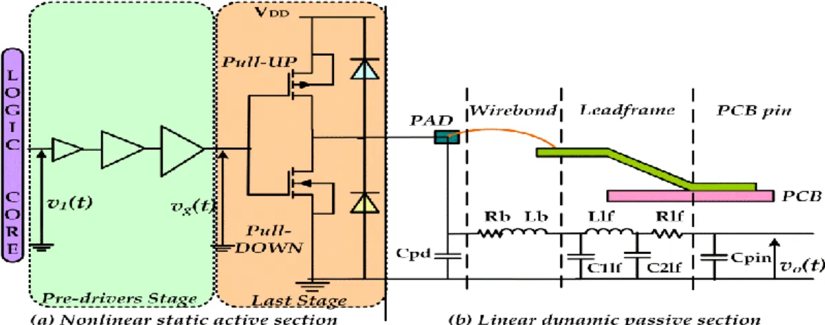
Figure 1.4 The two I/O buffer model sections: (a) Nonlinear active section and its main electrical variables. (b) Three-stages linear dynamic section of the package network. ... 3

Figure 1. 5. Ideal waveform at the logic core and Real waveform at receiving gate. ... 5

Figure 1. 6 Model hierarchy according to the physical details included in the model description and the design level [8]. ... 6

Figure 1. 7. Generic structure of the two-port I/O buffer with its relevant electrical variables. ... 8

Figure 1. 8. Behavioral modeling framework based on system identification theory. ... 9

e Figure 2. 1. One-port active network. ... 16

Figure 2. 2. General structure of a recursive ANN. ... 18

Figure 2. 3. Training scheme of an artificial neural network. ... 19

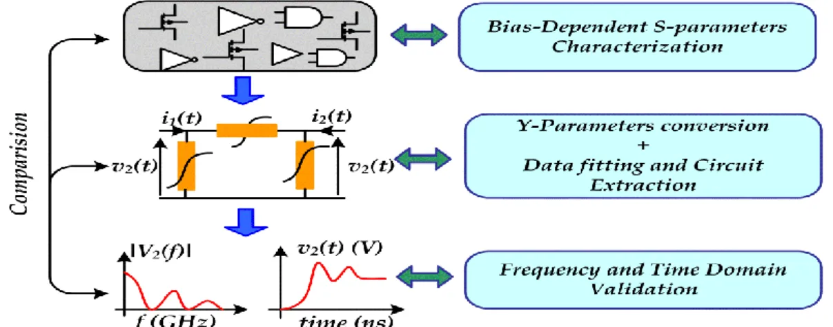
Figure 2. 4. Two port S-parameters characterization for the active device. ... 20

Figure 2. 5. Implementation diagram of the equivalent circuit extraction technique based on frequency domain measurements. ... 21

Figure 2. 6. Equivalent circuit nonlinear model with four state functions [16]. ... 23

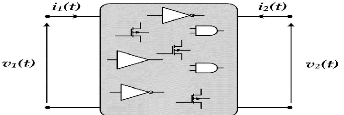
Figure 2.7. Basic structure of the two port I/O buffer and its main electrical variables. ... 25

Figure 2. 8. Key portions of the active intrinsic parts of IBIS model’s elements [25]. ... 27

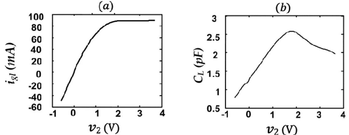
Figure 2. 9. Simulation setup for the generation the four I-V curves for IBIS model. The diodes start to conduct as exceeds the supply voltage bounds by an overvoltage . ... 28

Figure 2. 10. IBIS output buffer static I-V characteristics: (a) PD I-V curve, (b) PU I-V curve. 28 Figure 2. 11. Simulation setup for the transient identification signals when is kept at the high or the low logic state for each up and down transitions at the input . ... 29

Figure 2. 12. A functional form reproducing an observed electrical behavior of the device. ... 30

Figure 2. 13. Procedure for modeling the driver’s nonlinear dynamic function (.). ... 31

Figure 3. 1. One-port representation of the PU or PD devices of the driver’s last stage. ... 38

Figure 3. 2.Simulation setup for generating the driver’s identification signals for and . ... 40

Figure 3. 3. Model structure used in the identification of the two memoryless nonlinearities and for each local model. ... 40

Figure 3. 4. Time domain waveforms: (a) PWL signal, (b) ESS signal.(c) Spectrum magnitudes in dBv of the ESS, the PWL, and the pad voltage in mismatch loading condition. ... 43

Figure 3. 5. Comparison between the MSE convergences when the model of the driver’s PD last stage is trained with PWL(solide line) and ESS (dashed line). ... 43

Figure 3. 6. Single-valued nonlinear surface relates the output current to the output voltage and its first derivative (state variable). ... 43 Figure 3. 7. Static model’s functions of the PD last stage: (a) I-V function, (b) C-V function. . 44 Figure 3. 8. Comparison between the C-V functions extracted with ESS large signal (solid line) and the bias-dependent ac (dashed line). ... 44 Figure 3. 9. Model extrapolation (a) Comparison between the of the TL model (solid line) and the I-Q behavioral model (dashed line) when excited with a pulse. (b) The relative error with a much finer scale. The obtained NMSE was -30.08 dB. ... 45 Figure 3. 10. SI simulation setup used for the model validation. ... 46 Figure 3. 11. Validation of the I-Q behavioral model. The near-end voltage waveforms: (a)

Td=1.5ns and (b) Td=1ns. TL model response: solid line; I-Q model response: dotted line. ... 46

Figure 3. 12. Validation of the I-Q behavioral model. The far-end voltage waveforms: (a)

Td=1.5ns and (b) Td=1ns. TL model response: solid line; I-Q model response: dotted line. ... 47

Figure 3. 13. Comparison between the IBIS (dashed line) and the TL model (solid line) of the far-end voltage. ... 47 Figure 3. 14 Accuracy of I-Q and IBIS behavioral models is illustrated by the RE for each model in predicting the far-end voltage. ... 47 Figure 3. 15. Zoomed perspective of the first up transition of Figures 3.12.a and 3.14. IBIS model response: dashed line; I-Q model response: dotted line; TL model :solid line. ... 48 Figure 3. 16. Selected time instants of the duplicate amplitude of the for model extraction. ... 51 Figure 3. 17.Nonlinear dynamic characteristic of the output port of the lower and upper devices. ... 52 Figure 3. 18. Proposed model structure for the output behavior of an I/O buffer ( and are implemented as static LUTs). ... 52 Figure 3. 19. The mixed-model driver’s behavioral model circuit components within a CAD. . 54 Figure 3. 20. Conduction and displacement single valued nonlinearities for (a) the upper, and (b) the lower devices of the driver’s last stage... 55 Figure 3. 21. Comparison between the measured versus trajectories for the TL model, the proposed I-Q model and the model of [15]. ... 55 Figure 3. 22. Comparing the time-domain waveforms estimated by the TL model, the I-Q model and the model of [15]. ... 56 Figure 3. 23. Channel reflection setup used for the evaluation of the I-Q and IBIS models. ... 56 Figure 3. 24. waveform. Solid lines: TL model; dashed line I-Q model. ... 57

Figure 3. 26. Crosstalk validation setup with the RLCG coupled-line structure (Length=0.1m;

R11=R22=45.97/m,R12=5.23/m;C12=-17.69pF/m,C11=C22=317.72pF/m;L11=L22= 251nH/m, L12=41.38nH/m; G11= G12= G22= 0.00 S/m). ... 58

Figure 3. 27. Comparision between the near-end and far-end voltage waveform and on the active channel of Figure 3.27. Solid lines: TL; dashed lines: I-Q model. ... 59

Figure 3. 28. Comparision between the near-end and far-end voltage waveforms and

on the quiet channel of Figure 3.27. Solid lines: TL; dashed lines: I-Q model. ... 59

Figure 3. 29. Simulation setup for the extraction the bias-dependent Y-parameters data characterizing the upper and lower devices of driver’s output admittance. ... 61 Figure 3. 30. Extraction and comparison of the I-V function with dc measurements at the left side and the Q-V function at the right side. lower (a) and upper (b) devices’ functions. ... 63 Figure 3. 31. Crosstalk simulation setup used for the I-Q behavioral model validation. ... 63 Figure 3. 32. Comparison between the far-end voltage waveform on the active channel. Solid lines: TL model; dashed lines: I-Q model. ... 64 Figure 3. 33. Comparison between the IBIS and I-Q behavioral models against the TL model. Zoomed view of the far-end voltage waveform: (a) the first up output’s transition, and (b) the last down output’s transition. ... 64 Figure 3. 34. Validation of the I-Q behavioral model. The near-end voltage waveform on the quiet channel and the voltage error of the IBIS and I-Q behavioral models. ... 65 Figure 3. 35. Comparison between IBIS and I-Q behavioral models against the TL model in predicting the noise on the quiet channel. Zoomed view of the near-end voltage waveform: (a) the first up output’s transition. (b) the last down output’s transition. ... 65 Figure 3. 36 Generic digital I/O buffer electrical structure with its relevant electrical variables. ... 67 Figure 3. 37. SI evaluation setup for IBIS model under overclocking conditions. ... 69 Figure 3. 38. Comparison between the of the IBIS and TL models. (a) normal operation at a bit-rate of DR=350 Mbps and (b) overclocking operation at DR=800 Mbps. ... 69 Figure 3. 39. Step response characteristics of the pre-driver stage. ... 70 Figure 3. 40. Two-port circuit implementation of the digital output buffer. ... 72 Figure 3.41. Driver’s last stage simulation setup for the voltage-current gate effect identification. ... 72 Figure 3. 42.System’s representation of the Hammerstein model of the pre-driver’s stage. ... 73 Figure 3. 43. Simulation setup for the identification of and . ... 73 Figure 3. 44. Simulation setup for recording the transient identification signal for the filter parameters estimation. ... 74 Figure 3. 45. Nonlinear voltage-current functions for the output port PU and PD networks. ... 78 Figure 3. 46. Nonlinear voltage-current functions for upper and lower pre-driver’s stage. ... 78

Figure 3. 47. Circuit implementation of the FOPDT filters. ... 79 Figure 3. 48. Crosstalk simulation setup used for the two-port behavioral model validation. .... 79 Figure 3. 49. Validation of the two-port behavioral model for the test case #1, (a) on PCB trace #1 and (b) on PCB trace #2. ... 80 Figure 3. 50. Validation of the two-port behavioral model for the test case #2, (a) on PCB trace #1 and (b) on PCB trace #2. ... 81 Figure 3. 51. Comparison between the gate voltage waveform of the TL model and the one predicted by the pre-driver’s behavioral model for the test case #2. ... 82 Figure 3. 52. Eye diagram derived from the waveform of Figure 3.49 and the definition of the eye opening parameters and . ... 82 Figure 3. 53. Eye opening parameters of the waveform for the TL , IBIS model, and two-port behavioral model... 83

CHAPTER I:

Preliminaries and Backgrounds

This chapter presents a general introduction to the down-scaling trend in very-large-scale integration (VLSI) circuit and concepts concerning signal integrity (SI) and working mechanisms for digital communication systems. The classifications of various mathematical modeling approaches that can be used within the computer aided design (CAD) tools to evaluate the SI performance of a high-speed digital link are then described. Moreover, the need for suitable modeling of input/output (I/O) buffers characterized by their nonlinear dynamic behaviors for an accurate and fast prediction of SI is explained. This chapter ends by discussing the organization and the flow of the PhD thesis.

1.1

Introduction

Over the last decades, the continuing downscaling of the voltage supply, the high density integration, and the switching speeds of VLSI circuits have been increasing fast in the IC CMOS process in order to achieve high performance logic operation with reduced power and cost. As shown in Figure 1.1, the number of transistors per chip grows exponentially which reduces 25% the cost-per function every year in the ITRS [1]. It is worth to note that the ITRS partially uses historical trends to project the future of the semiconductor industry.

In addition, Figure 1.2 shows the trend of the clock frequency of microprocessors which had kept increasing until it reached 3 GHz. Although it has been decreased slightly down to 1–2 GHz when introducing the multi-core scheme, the local on chip and the core clock frequency is expected to keep increasing [1]. Consequently, the high frequency effects observed in the digital interconnected subsystems that were previously ignored in the model’s generation cannot be overlooked anymore and have to address these issues efficiently for accurate system level analysis [2], [3].

Figure 1. 2. Clock frequency trend for local on-chip (Core) and entire chip [1].

These circumstances have brought tremendous challenges to reliably transmit the data at high-speed. In fact, additional non-ideal effects may be generated and lead to severely distorted voltage and current waveforms and signal jitter, and result in faulty switching and logic errors [3], [4]. Consequently, the high-speed system’s design requires some additional efforts to overcome these issues by accurately predicting these effects in early design stages in order to ensure good signal integrity. This can be achieved by developing more efficient and accurate behavioral models for the main subsystems (i.e. I/O buffers) to capture their nonlinear dynamic behavior in order to evaluate the performance of the I/O signal quality in the whole high-speed digital link [5].

1.2

SI Simulation of Digital Transmission Link

The chip’s functionality is performed within the logic core. However, the I/O buffers are much larger than the core cells and they are required to bond the die to the package and the external interconnects. This transmission link within the IC introduces distortion into the propagating electrical signals. In fact, it can be decomposed as an

active part representing the I/O buffers that interface the logic core and the passive package and the printed circuit board (PCB) interconnects as depicted in Figure.1.3.

Figure 1. 3 Main parts of a generic of a high-speed digital interconnected system.

The I/O signals leave the chip #1 by means of an output buffer/driver characterized by a highly nonlinear dynamic behavior. After propagating through the IC’s package, and then the PCB, which are usually modeled as passive distributed transmission line elements, the signal reaches the chip #2 where the input buffer/receiver detects the transmitted input signal with the above mentioned imperfections according to the switching point voltage. A more detailed description of the I/O buffer enclosed in its package is shown in Figure 1.4.

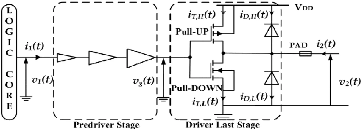
Figure 1.4 The two I/O buffer model sections: (a) Nonlinear active section and its main electrical variables. (b) Three-stages linear dynamic section of the package network.

In the active section, the last stage’s large transistors are arranged as a pull-up (PU) and a pull-down (PD) network. They impose the dominant electrical behavior of the device, while the pre-drivers stage act mostly as highly nonlinear voltage transfer characteristics followed by a resistive path feeding the gate capacitances of the last stage. On the other hand, the passive section structure is extracted from the associated small-outline IC package category [6] from Spectre simulator. The first element, ,

stands for the capacitance associated to the pad where the bond wire attaches the die to the package. After that, the quantities and are respectively the lumped bond wire inductance and resistance. In addition, the inductance , the coupling capacitances

and and the resistance represent the lead frame equivalent lumped model.

Finally, models the capacitive coupling between the lead frame solder pad and the

PCB backplane ground.

Therefore, in circuit-level simulation, the digital I/O buffer circuits have a major share in the computational load containing a very complex functional part and a high number of pins in the IC. Furthermore, due to the high switching frequency that is always being pushed to higher limits, and to the current intensity that is needed to source a generalized set of external ICs, output buffers are forced, in most cases, to distort the I/O signals due to their nonlinearity and dynamics. Thus, they constitute the IC bottleneck in terms of switching speed. In this concern, signal integrity (SI) is a very important task of ensuring sufficient fidelity of a signal transmitted between a driver and a receiver for proper functioning of the circuit (e.g., the signals over the high-speed bus between a processor and its chipset). A signal with good integrity characteristics is defined as one observed at the receiver within the desired time window and with adequate amplitude levels. The ideal voltage waveform in the perfect logic world and the distorted signal - in terms of amplitude and time deviations- by the active driver and the package dynamics of Figure 1.4 are illustrated in Figure 1.5 where the different manifestations of SI degradation are:

 A high logic voltage level lower than the minimum high acceptable level, ,

 A low logic voltage level higher than the maximum acceptable low level, ,

 Excessive signal delay - a rising/falling ( ) edge shows skews longer than the acceptable timing windows,

 Overshoot, undershoot and glitch - ringing and oscillation, long settling time. These effects are aggravated with the increase of the driver’s clock frequency and the mismatch load with external interconnects.

At the receiver’s input, voltage above the reference value is considered as logic high, while voltage below the reference value is considered as logic low. Any delay or amplitude’s distortion of the waveform will result in a failure of the data transmission. For instance, if the signal in Figure 1.5 exhibits excessive ringing into the gray zone while the detection occurs, then the logic level cannot be correctly received.

Figure 1. 5. Ideal waveform at the logic core and Real waveform at receiving gate.

According to this analysis, we conclude that the aim of SI analysis is to ensure reliable high-speed data transmission by evaluating three main issues. Firstly, the reflections that occur because of interconnect discontinuities such as impedance mismatch, vias, and other line discontinuities. Secondly, the noise induced by neighboring connections (crosstalk), produced in a signal line by other lines as inductive and capacitive coupling. Thirdly, the disturbance on power distribution by switching of the digital devices introduces a noise in a signal line that manifests itself by the voltage drop along the inductive path of the power supply network for the IC and its packaging. This noise is also called power and ground bounce, ΔI-noise or Simultaneous Switching Noise (SSN) [2], [3]. Hence, the performance evaluation of high-speed digital systems requires the accurate prediction of the waveforms propagating through the digital interconnects. Such prediction is usually carried out in a time domain simulation that allows the detailed analysis of the interactions between the digital IC peripheral devices (i.e. the input/output buffers’ impedances, and the loading interconnect traces).

In order to perform such simulations, a feasible strategy must subdivide the overall system in well-defined sub-systems typically found along the signal propagation paths, i.e., active devices, package, and transmission-line interconnects as illustrated in Figure 1.3. Each sub-system is separately characterized by a macromodel, i.e., a set of equations that are able to reproduce with sufficient accuracy the electrical behavior of the sub-system which is implemented in CAD library (e.g., SPICE-like, advanced design system (ADS), etc). Hence, modeling digital I/O buffer circuits to accurately capture their nonlinear dynamic behavior becomes a big challenge for SI performance evaluation of modern digital interconnected systems. This will result in an efficient use of CAD tools by providing the valid and appropriate large-signal behavioral models of the main connected sub-circuits [7].

The next section of this chapter outlines basic modeling approaches for the development of a driver’s a mathematical model suitable for system-level simulation by highlighting their strengths and limitations. Finally, the last section outlines how we can describe the driver’s behavioral parametric model using system identification theory.

1.3

System Identification Framework

1.3.1

Hierarchy of Modeling Approaches

As described in the previous section, modern high-speed digital communications systems are too complex to permit the complete simulation of the nonlinear behavior at the transistor level (TL) description. This model is the most accurate solution, and usually it is considered as the reference for the device. Unfortunately, the model completely discloses the internal details of the device. In addition detailed physical descriptions are generally large in size and their effect is to drastically slow down the simulation.

Finally, they cannot be easily plugged in any simulator, since they are usually written for a specific simulator in particular when encryption holds. This problem presents a significant productivity bottleneck for design engineers. A typical design and modeling hierarchy is depicted in Figure 1.6.

Figure 1. 6 Model hierarchy according to the physical details included in the model description and the design level copied from [8].

The modeling hierarchy begins at the bottom with the device model described by the detailed semiconductor physics. It ends at the top by a high-level abstraction that describes the terminal behavior through black-box or equivalent circuit behavioral functions. Since there are too many nonlinear interactions taking place at the system-level, the CAD simulation using TL models which is based on Newton Raphson

algorithm takes a long time to converge and uses too much memory to run [8]. A solution to this simulation bottleneck is to generate reduced-order behavioral models that describe the essential behavior of the complex active circuit blocks [9], [10].

Furthermore, behavioral modeling approaches can be classified according to the level of physical information used in the description of the model mathematical formulation (i.e. physically based (transparent) or black-box (opaque) model’s structure). Firstly, we have the black-box model that accurately describes the device’s experimental data by means of a high-level mathematical abstraction. The model simply solves a numerical fitting problem without reference to any underlying physics. Good examples of black box models are any form of parametric model based on artificial neural networks (ANNs) or other curve fitting techniques [11]-[13]. Secondly, the gray-box models which are parameterizations based on various degrees of physical insights. For instance, the large-signal equivalent circuit’s model composed of electrical elements such as resistors, capacitors, and nonlinear current or voltage sources, which can characterize the electrical properties of the active I/O buffers. The physically meaningful structure is determined by analyzing the recorded experimental data that carries the information on the device’s behavior and correlates it to the mechanism describing the device’s electrical properties by the physical reasoning and approximation theory [14]-[19].

Both the black-box and gray-box approaches use system identification theory tools to generate their model functions or to extract their parameters. They aim to enable circuit designers to capture high-level descriptions of modules and subsystems that speed-up the simulation and hide intellectual property (IP) while guarantying reasonable accuracy. Therefore, circuit designers can send their models to the system design team reducing overall time-to-market and thus generating additional revenues. The behavioral modeling framework will be described in the following subsections.

1.3.2

Device Characterization

When building a mathematical model to describe the I/O buffer’s circuit behavior, the model maker generally has two sources of information; a priori knowledge concerning the I/O buffers behavioral model properties (i.e. design circuit, application, and model structures) and a representative experimental data of the active device nonlinear dynamic effects. Furthermore, the performance of behavioral model’s construction is influenced by two key aspects: the observation and the formulation. The

observation refers to the accurate acquisition of the signals at the input and output ports of the device under modeling (DUM) while exciting the appropriate behavior as shown in Figure 1.7. The formulation corresponds to the choice of a suitable mathematical relation that describes all the significant interactions between the DUM’s input and output signals. Accordingly, sufficient background and a priori knowledge of the DUM is required to observe the right behavior and choose the adequate formulation.

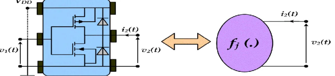
Figure 1. 7. Generic structure of the two-port I/O buffer with its relevant electrical variables.

The terminal currents and of the general two-port behavioral model for the general structure of Figure 1.7 can be expressed in time domain as a function of the two-port terminal voltages , , and their successive higher order derivatives

{ ( ) ( ) (1.1)

The system identification tool does not provide foolproof that always and directly leads to the optimum results. On the basis of the a priori knowledge, the excitation signal is designed to reflect the observed behavior under a specific excitation, the I/O buffer simulation setup is selected, the measurement procedure is specified and the operation range is defined. For instance, the model structure defined by the nonlinear multivariate functions (.) , has to be optimized and identified according to the following modeling framework as depicted in Figure 1.8, which has an interactive logical flow [20].

As arrows in Figure 1.8 point out, the model construction’s steps can be recursive and iterative. For instance, if the model’s accuracy is not satisfying, various model structures and identification signals should be tested and the process repeated. The characterization step considers generating a large-signal data by driving the DUM with

adequate excitation signal and record the time and/or frequency domain data that carry information on its behaviour. The data obtained from stimulation or measurement is processed and analyzed to fit the proper model structure.

Figure 1. 8. Behavioral modeling framework based on system identification theory.

It is worth noting that the DUM’s behavior can be attributed to many sources so that different simulation setups and excitation signal can be used to extract the adequate behavior and then combine them to construct the complete interaction between these effects. The gathered set of measurement results is a good representation of the device behavior only if the identification signal is properly designed to stimulate the nonlinear static characteristics and to excite all possible dynamics of the DUM. Thus, it should cover the frequency and magnitude ranges of interest which is important both for convergence of the behavioral model when used in the simulator. Besides, although the circuit terminations have no impact on the modeling process of linear circuit, the choice of terminations in nonlinear behavioral modeling directly affects the generalization property of the model. In fact, the model accuracy needs to be assessed by subjecting it to various boundary conditions (i.e. I/O signals or terminations). Finally, the resulted

model is implemented in the CAD library. More detailed descriptions of the model’s construction steps are presented in the following sub-sections.

1.3.3

Model Structure Formulation and Extraction

It is worth noting that behavioral modeling activities are not only restricted to replicate the I/O data with general curve fitting methods, that will be presented in subsection 2.2, for given infinite order and complexity [45]. In fact, it involves more challenging tasks as model structure formulation and optimization by means of nonlinear multidimensional function approximation to reduce the model identification and running complexities. This is achieved by analyzing the observed I/O signals, investigating the device physical design structure, and its operation under practical operation condition in order to develop a model that is coupled with measured quantities as it is the case of Input/output Buffer Information Specification (IBIS) that will be described in more details in the subsection 2.3.

Ljung summarizes this model structure formulation problem as follows: “This is no doubt the most important and, at the same time, the most difficult choice in the system identification procedure. It is here that a priori knowledge and engineering intuition and insight have to be combined with the formal properties of the models.” [9]. Furthermore, the model extraction heavily depends on the approximation methods used in the model formulation and the followed identification algorithm of its functions and parameters. In fact, model functions can be dependently extracted in order to minimize the complete model error [14]. It is worth noting that not only special care should be taken regarding the simulation setup but also the ability to perform the model extraction from laboratory measurements by collecting the required data from the available equipment and instruments. The recursive or direct model formulation depends on how deep the memory effect is exposed by the DUM behavior excited with suitable excitation signal.

1.3.4

Model Implementation and Validation

Once the adequate model structure and the corresponding identification algorithm are developed, the model must be exported to the format suitable for the use in most modern circuit simulators. It is worth noting that possible enhancements in behavioral modeling can be achieved by formulating them in language native to the simulator so it eases its implementation and interpolation by different circuit simulators.

Besides, the model validation involves various procedures to evaluate how the model relates to the measurement results and the intended usage. It amounts of verifying the correctness and the validity range of the behavioral model in the practical condition application by determining the correlation between the behavioral model’s and the TL model numerical results. This requires the selection of metrics to quantify the model accuracy while using boundary conditions (i.e. I/O signals or terminations) that have never been used in its extraction.

If the model fails to meet the selected requirements, the model’s identification procedure has to be restarted from an earlier step as shown in Figure 1.8. Various factors can lead to a deficient model:

 The driver’s measurements do not provide sufficient information or are too noisy.

 The selected model structure (i.e. linear vs. nonlinear) is inappropriate to represent the driver’s behavior.

 The chosen order (i.e. number of basis function and the memory length) of the model is too low or too high.

 The model’s identification algorithm failed to correctly extract all the parameters.

The model’s extrapolation assesses the predictive capabilities of the constructed model by subjecting it to excitation signal’s magnitude and frequency ranges higher than the one used in the characterization and extraction steps while loaded by different terminations. In such case, the implemented model’s convergence during the transient simulation should be also verified. This is because simulators solve nonlinear algebraic equations using iterative algorithms such as Newton’s method and it may happen that, in the process of convergence, the iteration takes a step where the independent model variables go outside the region of validity. In fact, the simulator extrapolates the value of the dependent variable (output of the model) according to the definition given for the functions , in (1.1) and cannot encounter the solution of the nonlinear numerical problem and thus will never converge.

1.3.5

Summary

The evaluation of the signal integrity is of a paramount importance with the recent trends in VLSI design characterized by the downscaling of the package integration and the clock frequency. As a result, the number of failures caused by SI problems is on the

rise because existing modeling methodologies for I/O buffers cannot address these issues effectively.

Since the correct operation of I/O buffers is crucial to reliably transmit data through high-speed digital links, developing an efficient model to accurately simulate their nonlinear dynamic behavior is a challenging task that is motivating several research activities [11]-[15]. In fact, the previously neglected nonlinear dynamic effects in the active I/O buffers should be captured in the supplied model to the designer in order to accurately perform time domain simulation.

In order to overcome the TL limitations, behavioral modeling appears to be effective. Such high-level abstractions are developed to characterize the device behavior by subjecting it to various types of excitation to find out the different sources of nonlinearity and dynamics and their effects on device’s behavior. This enables fast and accurate prediction of magnitude and timing waveform quality degradation due to these physical imperfections. Such behavioral models can be classified in two types according to the physical knowledge reflected in the model generation’s process (i.e. the black-box and gray-box techniques).

1.4

Thesis Contributions and Dissertation Outline

According to the new paradigm in the integrated electronic system and the available approaches for circuit descriptions of the output buffers/drivers switching properties in modern simulators, this doctoral thesis is focused in the construction of analog behavioral models of the nonlinear dynamic high-speed drivers enabling efficient simulation and evaluation of SI performance. In fact, modeling the input buffers/receivers is considered as a simpler case of the drivers’ modeling problem and its resulting behavioral models can be extended to model the receiver case. This PhD work is centered on the system identification framework to improve the previously published behavioral modeling [11]-[15]. In fact, the model should balance the accuracy/complexity trade-off which requires profound knowledge of device nonlinearity, circuit design, and nonlinear characterization tools and model formulations.

This work will contribute to reduce the order of nonlinear parametric models [11], [12] and enhance the equivalent circuit IBIS model’s structure [13]-[15] by merging the features of the black-box and gray-box driver’s behavioral modeling generation. Moreover, a completely new physically inspired behavioral two-model mathematical

formulation extraction and implementation is generated for simulating the driver’s behaviors in overclocking operations. These achievements have an important impact to ease the design of the future high-speed digital link by providing effective numerical models of memory I/O interfaces for better simulation performances within the CAD tools.

The remainder of the thesis is organized as follows.

Chapter 2 gives an overview of the common mathematical modeling and function approximation techniques used in nonlinear driver’s behavioral modeling approaches. It also outlines other possible appealing techniques that will be used in improving the previously published approaches and eases the understanding of the achieved results in Chapter 3. Particularly, the general curve fitting and the equivalent circuit-level functions are detailed by discussing their strengths and limitations.

Chapter 3 describes the developed research work that aims improving both the state-of-the-art IBIS and the nonlinear parametric modeling approaches by presenting a physically meaningful empirical model to capture only the one-port driver’s last stage output port behavior along with their different extraction procedures and implementation. In the chapter’s last section, an optimum and physically inspired two-port analog behavioral model for accurately capturing the driver’s operation in overclocking conditions is developed.

Finally, Chapter 4 provides the main conclusions that can be drawn from the achieved results of the PhD thesis and presents the possible future work.

CHAPTER II:

Driver’s Behavioral Modeling Methodologies

2.1

Introduction

Measured or simulated nonlinear behavior can be expressed by a series of equations in time or frequency domain using voltages, currents or incident and reflected waves at all ports. If one performed an infinite number of measurements by changing the environment (i.e. power supply levels, biases, load impedances, etc.), the resulting infinite table of realizations would describe this device completely. Clearly, this is not an option. However, performing a finite set of observations that can be interpolated with confidence using mathematical modeling and function approximation is more practical.

With the aim of analyzing the origins of behavioral modeling developed for output buffer/driver to capture its nonlinear and memory effects and in a way to establish a link with their modeling approaches through large-signal equivalent circuit model and parametric curve fitting techniques, a comprehensive overview of the mathematical modeling framework based on system identification theory is presented in this chapter. For sake of simplicity, the methodology is firstly described for one-port active devices. Then, it is extended to two-ports covering the black-box and the gray-box formulations and identification for modeling the driver’s nonlinear dynamic behaviors where the state-of the-art Input/output Buffer Information Specification (IBIS) and parametric modeling are analyzed and discussed.

2.2

Mathematical Modeling and Function Approximation

Device simulators such as ADS [40] or SPICE [43] require that terminal currents are expressed in some functional form. Parametric behavioral models are based on approximating the device’s behavior by a simpler function over some defined region and to some specified accuracy. When a function is fitted to measured data, various candidate basis functions can be selected from a large set, such as the polynomial family, rational functions, splines, and neural networks which are discussed in [10]. Besides, the function parameters are adjusted by a proper algorithm until the data is represented with sufficient accuracy over the measured data space.

In one-port networks, the input and output signals (i.e. voltage, current or incident and reflected waves) that enter and exit the one terminal are shown in Figure 2.1.

Figure 2. 1. One-port active network.

In a memoryless or static system, - in which no charge or magnetic flux storage elements (no capacitors or inductors) exist, so that the voltages and currents at any instant do not depend upon previous values of voltage or current-, the output of the one-port device, , can be uniquely defined as a function of the instantaneous input signal , and the model can be reduced to or since the dependence on time is immaterial. However, the output buffers, as all active electronic circuits, present memory effects and thus they are said to be dynamic. The output now depends also on the input, or output past and system state. The input-output relation becomes an operator that maps a function of time onto another function of time . Thus, the input–output mapping of the device can be represented by the following forced nonlinear ordinary differential equation (ODE) [21]:

[ ] (2.1) This states that the output and its time derivatives can be nonlinearly related to the input and its time derivatives. By assuming the back-ward discrete-time approximation of the continuous-time derivative of a signal :

( ) ( ) (2.2) the discrete time version of (2.1) can be expressed in the recursive form:

The sampling period is , so that the time corresponds to the discrete variable such as: . Also, the input-output signals such as, . Here is the present output at time instant . It depends in a nonlinear way, on the output past , the present input , and its past . Nevertheless, under a broad range of conditions (basically, operator causality, stability, continuity, and fading memory), such a system can also be represented with any desirable small error by a non-recursive, or direct form, where the relevant input past is restricted to { }:

[ ] _(2.4) Similarly, the behaviors of active devices, (e.g. I/O buffers) encountered in the high-speed digital communication link are described by nonlinear ODE. The behavioral modeling task consists in capturing the essential observed dynamics by constructing the function which maps the ( ) independent variables into the dependent variable. This function can have a direct or recursive formulation, and , respectively. In the following subsections, the parametric black-box and the gray-box modeling methodologies used in fitting and representing the nonlinear functions and , respectively, will be presented. Accordingly different identification procedures and model descriptions in time or frequency domains will be analyzed.

2.2.1

Parametric Functions

In the first case, the direct form of a memory polynomial that interpolates functions can be written as:

∑ ∑ ∑ ∑ ∑ (2.5)

where the are the memory polynomial coefficients that can be estimated in a direct way by a simple least-squares method. The last equation can be written in matrix form in which is the vector of the model coefficients, is the vector

of the output data samples and is the matrix that contains the mixture elements of the input signal . The least-squares method can be used to find the polynomial coefficients:

_(2.6)

where denotes the conjugate transpose of the matrix . Although simple in concept, this finite impulse response (FIR) polynomial model architecture is known for its large number of parameters. For similar approximation capabilities and many fewer parameters, the recursive polynomial infinite impulse response (IIR) structure can be used, but its stability should be verified at the model extraction and validation steps.

In the second case, the functions are built using the ANNs. The recursive structure is illustrated in Figure 2.3 in which the dynamic mapping depends on the past values of both the input and output signals.

Figure 2. 2. General structure of a recursive ANN.

The ANN input-output mapping, with N neurons, and { } dynamic order for the input and the output respectively, is mathematically described by:

{ ∑ ∑ ∑ (2.7)

where , , , are weighting coefficient, and are bias parameters and (.) is the activation function. Figure 2.2 shows that the model output is built from the addition of the activation functions and the weighted outputs. The inputs are biased sums of the various delayed version of the input and output weighted by the coefficient and , respectively. The ANN model is nonlinear in the parameters and and linear with

respect to the parameters and . Various nonlinearities, , can be used as activation functions. For instance, the hyperbolic tangent function is defined as:

(2.8)

The ANN’s activation functions are bounded in output amplitude. Thus they do not share the catastrophic degradation of polynomials outside the training zone, during circuit simulation that could escalate to divergence problems.

Since, the ANNs model is usually considered as nonlinear with respect to all its parameters [22], a nonlinear least-squares algorithm is used for training by minimizing the Mean Square Error (MSE) cost function between the model and the TL outputs as shown in Figure 2.3. This means to find:

| { ∑ ̂

} (2.9)

where ̂ is the sampled output signal, is the total number of samples and is the response of the model to the sampled input signal . The sampled identification signals must contain all the information of the original signals. Therefore, the sampling period must be smaller than the sampling time defined by the Nyquist frequency of the identification signals. On the other hand, should not be too small, in order to avoid oversampling and consequent numerical problems in the minimization of (2.9). As a rule of thumb, the ratio should be on the order of 2÷6.

It is worth to note that the problem (2.9) is nonconvex and the solution obtained by means of the optimization algorithm can fall into local minima of the cost function. Thereby, a good initial estimate of the model’s parameters is crucial, since the initial starting point determines in which local minima the algorithm will end up which will affect the model generalization capabilities [22], [23].

The ANNs and the polynomial expansion have been proven to universally approximate any continuous multivariate function with any degree of accuracy provided that enough neurons and dynamic orders are considered which defines the number of the ANN’s weights and bias coefficients, and so its complexity. However, there is no way to know a priori the numbers of neurons or dynamic orders required for representing a specific system or the modeling improvement gained when these parameters are increased. In addition, the black-box recursive ANNs models suffer also from instability issues while the training or circuit simulation and from over-fitting during model’s identification.

2.2.2

Scattering Functions

For linear dynamic devices (e.g. filters, package, linear amplifier, etc.), S-parameters provide a black-box behavioral model in frequency domain. They are small signal representation of the transmission and reflection coefficients of a DUM at the input and output ports, and are defined in terms of a given reference source and load impedances, usually 50 , as shown in Figure 2.4.

Figure 2. 4. Two port S-parameters characterization for the active device.

The two-port DUM’s reflected waves and can be related to the incident waves and at the input and output ports, respectively, by the S-parameter matrix:

{ [ ] [ ] [ ] (2.10)

In the large-signal case some of the energy is reflected and transmitted at harmonics of the fundamental frequency. The S-parameters can be extended as a function of the DC bias point and the measurement frequency. We can also introduce

the port indices i and j and write the two port equations in summation. The S-parameter dependence on bias point and frequency of the source frequency is expressed as:

∑

(2.11)

The recorded large-signal and frequency-domain data from the TL simulation, or tailored measurement setup performed with a Vector Network Analyzer (VNA), of the active DUM (e.g. a diode or MOSFET transistors) can be fitted to an equivalent circuit model in terms of resistors, capacitors, inductors, and voltage controlled current sources or voltage controlled voltage sources, etc. In fact, the measured S-parameter data are converted into Y-parameters. Then, the circuit is extracted by fitting the data into the adequate equivalent network structure for the input and output ports. Finally, the overall equivalent circuit can be run in a SPICE based tool, and the S-parameters can be calculated and compared with the measured values. The implementation of this extraction technique is outlined in Figure 2. 5.

Figure 2. 5. Implementation diagram of the equivalent circuit extraction technique based on frequency domain measurements.

Qualitative and quantitative considerations on the validity of the circuit models extracted can be drawn by simulating the large-signal frequency domain (e.g. Harmonic Balance) to compare the output spectrum and transient response (e.g. SPICE) to compare the time domain signal or the eye-diagrams.

The large-signal equivalent circuit structure that fits the frequency domain data can be proposed based on the physically knowledge considerations. This approach will be described in more details in the next subsection 2.2.3. The equivalent-circuit constructed model will help the semiconductor designer to evaluate the impact of the

device characteristics affecting transmitted signal properties such as amplitude and timing distortion. These measurement-based models are usually implemented as simple look up tables (LUT) which are interpolated for any input condition to perform SI simulation. The constructed model balances the trade-off between accuracy and complexity and avoids the difficulties in model structure selection and/or its parameter estimation.

2.2.3

Equivalent Circuit Based Functions

An alternative approach to describe the model structure is based on the I/O buffers equivalent circuit or the device physical properties. Its topology is usually derived from direct inspection of the driver’s physics while the value of its parameters or functions can derived from gathered measurement and system identification theory in order to generate a physically meaningful model. This is particularly evident by investigating the way how active devices are modeled by nonlinear lumped or distributed circuit elements. As a result, these equivalent circuit based driver’s behavioral models are the consequence of a conscious combination of black-box behavioral and physical (e.g. white-box) modeling approaches. It can be seen as gray box modeling approach which naturally produces more efficient behavioral model by enhancing the accuracy level and reducing the complexity of the black-box model.

Since, the driver’s behavioral models are expected to predict port mismatches and timing and amplitude distortions in SI simulation, they must be able to represent in the time domain the port’s voltage and current or incident and reflected wave relationship in frequency domain. Therefore, their topology is of double-input double-output nature. This is a generalization of single-input single-output recursive or direct models of equations (2.3) and (2.4) of the one-port representation of the first example in the previous section 2.2. If the input and the output are components of the incident and reflected wave respectively, then equations (2.3) and (2.4) represent a nonlinear generalization of the linear scattering matrix. If they are stated as voltages and currents, we end up with a nonlinear generalization of the nonlinear admittance or impedance matrix formulation.

To illustrate the principle, the two-port large-signal model of a MOSFET is considered as represented in Figure 2.6. The intrinsic terminal behavior can be specified by the voltages and and current and at ports 1 and 2, respectively. To be complete, the extrinsic elements, as well as the non quasi-static effects should normally

be added. The simplified scheme consists of the parallel connection of a charge and current source at both port 1 and port 2. They are the device’s state-functions that reproduce the two ports electrical behavior and can be extracted based on equivalent circuit or black-box model identification providing large-signal data from time domain or frequency domain measurements [17].

Figure 2. 6. Equivalent circuit nonlinear model with four state functions [16].

The terminal currents can be expressed in the time domain by:

{

( ) ( )

( ) ( ) (2.12) and the displacement current at the input and output ports are defined as follows:

{ ( ) ( ) ( ) ( ) (2.13) Defining: { ( ) ( ) ( ) ( ) ( ) ( ) ( ) ( ) (2.14)