Shrubland fire behaviour modelling with microplot data

Shrubland Fire Behaviour Modelling with Microplot Data

Can. J. For. Res. 30: 889-899 (2000)

Paulo M. Fernandes1. Secção Florestal, Universidade de Trás-os-Montes and Alto Douro, Quinta de Prados, 5000 - 102 Vila Real, Portugal. Tel. (351) 259350236; Fax (351) 259350480; e-mail [email protected]

Wendy R. Catchpole. School of Mathematics and Statistics, University College, ADFA,

University of New South Wales, Canberra, ACT 2600, Australia. Tel. (61) 2 62688890; Fax (61) 2 62688886; e-mail [email protected]

Francisco C. Rego. Estação Florestal Nacional, Tapada Nacional das Necessidades 1300

Lisboa, Portugal. Tel. (351) 213973206; Fax (351) 01 3973206; e-mail [email protected]

1

Author to whom all correspondence should be addressed.

Abstract: Fire behaviour modelling has been based primarily on experiments involving the

measurement of a certain number of fires, where each variable is represented by an average value per fire. The main objective of this study was to examine if data collected from a microplot sampling design could be used to derive meaningful fire behaviour models. Three burns were conducted in low shrubland of Erica umbellata Loefl. and Chamaespartium tridentatum (L.)P. Gibbs in NE Portugal. Wind speed and aerial dead fuel moisture content varied from 5 to 27 km hr-1 and 14 to 21% respectively. Rate of spread and flame length ranged from 0.3 to 14.1 m min

-1 _{and 0.2 to 3.1 m respectively. Rate of fire spread could be described effectively in terms of an}

empirical model with wind speed and fuel height as independent variables. The coefficients that describe the effects of wind speed and fuel height on fire propagation were consistent with published values for similar fuel types. Flame length was strongly related to Byram's fireline intensity. Microplot sampling is not free from methodological problems - which are discussed - but can be effectively used in field studies of fire behaviour.

Introduction

Most fire management activities are based on fire behaviour prediction systems. Field experiments to validate or develop fire behaviour models involve numerous burns in order to include the widest variation possible of the relevant variables and produce reliable relationships. For example, Andrews (1980) reported four studies that examined the performance of Rothermel's (1972) fire spread model where the number of observations ranged from 10 to 42. Hunt and Crock (1987) used data from 88 prescribed burns in Pinus elliottii stands to test the fire

behaviour predictions given by an Australian burning guide. Between 8 and 63 fires were used per conifer fuel type to relate rate of spread with the Initial Spread Index of the Canadian Forest Fire Danger Prediction System (Forestry Canada Fire Danger Group 1992), although several observations were used in more than one fuel type. Marsden-Smedley and Catchpole (1995) used 52 experimental burns and wildfires to derive their fire behaviour models for buttongrass moorland, and tested the models with data from nine burns.

The problem of estimating fire rate of spread under nonuniform fuel conditions has been recognized and addressed (Frandsen and Andrews 1979, Fujioka 1985, Catchpole et al. 1989), but few experiments take advantage of the existing heterogeneity. Regression analysis of fire behaviour data generally uses only one value per experimental fire for each fuel variable. However, data describing within plot variability of fuel or fire behaviour is frequently available, such as in the following examples. Nelson and Adkins (1988) made 7 to 15 measurements of flame characteristics during each burn, Cheney et al. (1993) sampled fuel load and depth on a 16 point grid sample in each plot, and Marsden-Smedley and Catchpole (1995) collected fire behaviour information on 5 to 15 locations per fire.

Nelson and Adkins (1988) suggest localized fire and fuel measurements as a way to strengthen correlation results in fire behaviour modelling. Marsden-Smedley and Catchpole (1995) tried to match rates of spread during time intervals to the corresponding wind speeds measured by a weather station located near the edge of the plot, but could not get good correlations. In fact, because of spatial and temporal wind field variation, remotely placed anemometers may not properly reflect the wind acting directly on the flame zone (Cheney et al. 1993).

A few authors have used individual plots within a burn as sampling units of fire behaviour or effects. Simard et al. (1984) used 9 m2 _{plots, and were able to stratify fire spread data of a}

prescribed burn in two significantly different groups. Ryan and Noste (1985) rated fire severity of prescribed burns using 0.25 m2 plots located along a transect. Hawkes (1986) measured fuel consumption with transects that were laid out within 7 m2 _{circular microplots; a comparison of}

estimates at the microplot and large plot levels did not reveal significant differences. Smith et al. (1993) measured all fuel, fire behaviour and fire effects variables in small plots of 0.75 m2

within burns. Their study shows that microplots describe pre-burn conditions and fire behaviour as accurately as macroplot (whole burn area) methods, and they succeeded to relate fire behaviour variability to fuel characteristics. They concluded that microplot data can be used in correlation studies, thereby reducing the number of experimental burns needed, and improving the range of collected data.

No examples of fire behaviour models developed from microplot data are known. The main objective of this study is to examine whether microplot sampling schemes can be applied to empirical fire behaviour modelling in shrubland vegetation. A secondary objective is to obtain insights on the most suitable fuel variables to use in a shrubland fire spread model.

Experimental methods

Study sites and experimental design

The study was conducted in northeastern Portugal. Two plots designated as site 1 and site 2, respectively at the altitudes of 970 m and 850 m, were selected in the Padrela upland at 41o _27'

N and 7o _{30' W. The average rainfall in the area is approximately 1000 mm year} -1 _{and the mean}

annual air temperature is 12oC (Agroconsultores-COBA 1991). A third plot (site 3) was located in the Marão mountains (41o 17' N, 7o 44' W) at an elevation of 1250 m, where annual precipitation is approximately 1200 mm and the mean annual temperature is 11o_{C. The plots}

were rectangular and measured approximately 0.3 hectares in sites 1 and 3, and 0.7 hectares in site 2.

All sites are flat and occupied by low mediterranean heathland of the Ericion umbellatae alliance (Rivas-Martinez 1979), growing in oligothrophic soils underlain by schists. The stands are dominated by the heath Erica umbellata Loefl. (EU) and the shrub Chamaespartium tridentatum (L.)P. Gibbs (CT).

The stands were selected in order to typify the development phases of the EU-CT shrubland (Fernandes 1997): building on site 3, aged 5 years; mature on site 2, aged 14 years; and senescent on site 1, aged 18 years.

The hexagonal shape of the microplots used by Smith et al. (1993) was retained in this study since it allows fire behaviour observation across a nearly uniform distance regardless of fire propagation direction. The microplots measured 1 m2 _{and were marked with 1 meter stakes}

joined by white string around the perimeter.

The microplots were evenly spread along the longitudinal axis of the experimental sites, and homogeneous vegetation - continuous in cover and uniform in height - was sought for their location, since low structural variability within an observation unit is likely to help the analysis of fire behaviour. As a result, the distance between two consecutive microplots ranged from two to five meters. The number of microplots was 22 in site 1, 25 in site 2 and 10 in site 3.

Fuel sampling

Characterization of the fuel-complex structure was detailed but non-destructive. Pre-burn microplot sampling involved the measurement of height and percentage ground cover for CT and EU, and a visual assessment of fine dead fuel percentage for each species. Herbs and the other shrub species were disregarded because their cover never exceeded 2 per cent in the few microplots where they were present. Height was taken as the distance between litter and the top of the shrub crown, and was measured to the nearest 1 cm; the average height per species was calculated from six readings, one per each of the triangles circumscribed by the hexagon. Overall microplot height was determined by weighting the height of each species by its respective cover.

EU litter has a bulk density of 66 kg m-3 and a packing ratio (volume fraction of fuel) of 27% (Fernandes 1997) and was judged uncapable of sustaining flaming combustion. Litter from CT is much more aerated, with a bulk density of 23 kg m-3 and a packing ratio of 5%, and was considered available fuel for fire propagation. Specific equations for the study region (Fernandes

and Rego 1998a) were used to estimate both CT litter and aerial fuel loadings. CT litter is comprised of fine fuels (less than 6 mm in diameter) only. Aerial fuel was quantified for each shrub species, size class (<2.5 mm, 2.5-6 mm, >6 mm), and live and dead condition. The sub-division of fine fuels in two size classes is in agreement with European fuel characterization standards (Valette et al. 1996).

Analysis of variance was used to determine if the three sites were different regarding their fuel characteristics, by comparing the means with the Tukey-Kramer HSD test. The significance level was set at p<0.05; this p-value applies to all analysis made in the study.

Fuel moisture

Fine fuel samples for moisture content determination were taken just before ignition. Thirty dead fuel samples - ten for litter and ten for the canopy of each shrub species - were randomly collected in site 2. An identical procedure was followed in site 3, but litter was very scarce and it was not collected. The presence of maritime pine (Pinus pinaster Ait.) trees near some microplots caused heterogeneous shading conditions over site 1, which motivated the increase of sampling intensity for dead fuels. Three samples - one per fuel category (EU, CT fuel, and litter) - were collected in the vicinity of each microplot. Ten live foliage samples (five for each species) were taken on each site.

The fuel samples were sealed into plastic bags and oven dried at 85o_{C for 48 hours. Fuel}

moisture content was expressed as a percentage of dry weight.

Average live moisture content was estimated for the microplots of all sites by weighting the average site values of the species by their live loads in the microplots. The same approach was followed to estimate aerial dead fuel moisture content, using plot averages (sites 2 and 3) or the values obtained from sampling at the microplot level (site 1). Estimates of the average (or overall) dead fuel moisture content in the microplots were also made as weighted averages of

aerial and litter moisture content; equal water contents were assumed in site 3, where vegetation was much lower and litter quantity was negligible.

Weather data

Air temperature and relative humidity were registered for reference just prior to ignition, using a meteorological station located near the edge of the plots.

Surface wind speed was recorded at 2 meters height with a hand-held digital cup-type anemometer, by an operator who accompanied the fire front movement. The measurements were taken upwind and as close to each microplot as possible, but away from indraft influences of the fire. Three wind speed assessments (each one an average of 10 seconds) were taken at each microplot whenever possible, because the time available for measurement is inversely related with rate of spread. Only one or two wind speed values could therefore be acquired in the observation units that experienced higher fire spread rates.

Burning procedure

The experimental plots were burned during the winter of 1995. The fires were lit 10 meters ahead of the first microplot and ignited with a drip torch along the windward edge of the plots. The ignition line was perpendicular to the prevailing wind direction, which roughly coincided with the microplots axis. Ignition lines of 50 m on sites 2 and 3 and 30 m on site 1 (due to plot constraints) were considered lengthy enough to quickly reach quasi-steady rate of spread, given the low to moderate burning conditions under which the experiments were carried (McAlpine and Wakimoto 1991, Cheney et al. 1993, Cheney and Gould 1997).

A burned control line was established along the downwind edge of each plot. Previously existent natural and artificial barriers obviated the necessity for other fire control operations. Fire behaviour data and calculations

Two observers with chronometers, one on each side of the fire, registered the time the flame front base moved into each microplot (t1), and the time it reached its opposite side (t2). Their results did not differ significantly and were averaged to calculate rate of spread (R, m min

-1_):

[1] R = 1.24

t₂− t1

where 1.24 is the distance (m) between two opposite sides of 1 m2 hexagon.

A third observer visually assessed flame geometry, using the microplot poles as a reference: height from the ground surface to the top of the main flame, and angle between the frontal edge of the flame and the horizontal. Height was estimated to the nearest 0.2 metre for flames up to two metres high, beyond which estimates were made to the nearest half metre. Angles were visually estimated to the nearest 15o, with vertical flames being assigned 90o. Three estimates were made, one per each third of a microplot, and then averaged. The measured flame height was adjusted by subtracting vegetation height, and flame length (L) was calculated as (Alexander 1982):

[2] L = hF

sin A where hF is flame height and A is flame angle.

Flame length interpretation follows Nelson and Adkins (1986) and Catchpole et al. (1993), being less subjective than the conventional definition that implies a measurement of flame angle from the middle of the combustion zone, and therefore is highly dependent on flame depth evaluation. It is also likely to be more related with the fuel array being burnt in the microplot.

The fires were video recorded for further checking of fire behaviour data.

Fireline intensity (I, kW m-1_{) was calculated according to Byram's (1959) equation:}

where h_c is the heat yield per unit mass of fuel (kJ kg-1_{), w is the weight of the fuel available to}

combustion (kg m-2_{) and R is the rate of fire spread in m s}-1_{. The high heat of combustion of CT}

and EU is 22,500 kJ kg-1 _{(Gomes 1982), which was reduced by 1,263 kJ kg}-1_{, and by 24 kJ kg}-1_,

respectively per moisture content percentage point to obtain hc (Alexander 1982). Fuel consumption was estimated from a post-burn inventory at the microplot level that measured the percentage of canopy cover of the remaining foliage and, following the suggestion of Gill and Moore (1994), the terminal diameters of 10 twigs or stems; a value of 1 mm was assigned to partially consumed leaves. The following computations were then performed:

[4] w_2.5= W

(

)

(

)

where W and w are respectively the preburn and postburn fuel loads (kg m-2_{) in the <2.5 mm and}

2.5-6 mm size classes, C is the fractional post-burn cover, and dt is the average terminal twig and stem diameter (mm). and were disregarded in the The calculation of fireline intensity disregarded litter, whose consumption would be very difficult to estimate, and fuels larger than 6 mm, that burned only in a few microplots of site 2.

Experimental results

Fuel and weather conditions

Mature communities of the CT-EU shrubland type - whose fuel characteristics are described in Fernandes (1997) - are highly flammable and can accumulate up to 20 t ha-1 _of

aerial fuels, but litter is discontinuous and hardly reaches 2 t ha-1_.

EU dominated the microplots of site 1, CT was largely predominant on site 3, and there was an equilibrium between species on site 2. Table 1 displays the variables that were measured

to characterize the microplot fuel-complex, as well as overall descriptors (overall height, total cover, and dead fuel percentage) that were calculated from the former. The corresponding estimated fuel weights by size class and condition are given in Table 2. Microplots in site 3 were significantly different from microplots of sites 1 and 2 for the variables in Tables 1 and 2, with the exception of total ground cover percentage, and both EU and overall dead fuel percentages. Sites 1 and 2 differed significantly only in average EU cover and dead fuel percentage of EU and CT.

Weather conditions during the burns are given in Table 3. All burns were conducted under clear sky conditions. Windspeed covered a wide range of values within each fire, with coefficients of variation of 28% in site 1, 33% in site 2 and 40% in site 3. Sudden shifts in the direction of wind occurred when site 1 was being burnt.

Dead fuels were wetter - due to higher relative humidity - and exhibited a marked vertical profile in site 1, as an outcome of the reduced number of days since last rain (Table 4). Live fuel moistures on sites 1 and 2 are within the typical range for this vegetation type during the dormant season; the higher value on site 3 can be explained by its age (Fernandes 1997) and beginning of the spring green-up (Viegas et al. 1992).

Fire behaviour

As found by Smith et al. (1993) no changes in fire behaviour that could be attributed to fuel compaction caused by the preburn inventory were observed when the flame front moved into the microplots. Tables 5 and 6 display the observed and computed fire behaviour and fuel consumption parameters, excluding 13 microplots - seven in site 1 and six in site 2 - that experienced modifications in wind direction or for which poor visibility resulted in uncertain measurements.

Each burn attained a different level of fire behaviour. Propagation was poorly sustained at low windspeeds in site 1, presumably because of the relatively high dead fuel moisture content.

In site 3 the fire advanced with difficulty and fuel consumption was very incomplete. The site 2 burn, on the contrary, was characterized by an intense fire front that entirely removed the fuels <2.5 mm. Elevated fuel, rather than litter, was the vector of fire propagation on all sites. Fire behaviour descriptors varied greatly within burns, with coefficients of variation greater in site 3 (82% for rate of spread and 51% for flame length) and varying in the 41-72% range for the other sites.

Statistical modelling

Fire behaviour analysis

Microplots from the same site naturally tended to be more similar than microplots from different sites. Site effects include differences in fuel age, season of burn, species composition, altitude, and environmental conditions at the time of the fire. Thus there are two sources of experimental variation, between sites and within sites. To obtain a predictive model of spread rate, applicable to other sites, the site effects must be regarded as random variables from a population of possible sites.

It is common for variability in spread rate data to increase with mean spread rate (see for example Cheney et al. (1993) and Marsden Smedley and Catchpole (1995)). Thus we considered a linear model relating the logarithm of spread rate to functions of the fuel and environmental variables. This model can be written in the form

[6]

ln(R) = b

+

∑

b

V

+ S

+

ε

where R is the spread rate, and V_k is the value of the kth

independent variable at the jth

microplot on the ith

site, S_i is the site effect of the ith

site, ε(ij) is a random variable associated with the ith

microplot on the jth

site, the bk (k = 1 ... m) are constants, and m is the number of independent

variables used in the model. Microplot variables, or combinations of variables, considered were ones that might be expected to have an influence on fire behaviour, such as plot height, total

cover, plot height times covered area (volume), percentage cover of CT compared with total cover, and percentage of dead fuel in the plot.

It might be considered possible to analyse the data assuming the site effects as fixed effects, establish which variables contribute most to variations in spread rate, and then test whether site effects are significant after these variables have been included in the model. The problem with this is that variables affecting spread rate may be correlated with sites effects. Suppose, for example, that one of the variables has no effect on rate of spread, but is spuriously correlated with site effects that do affect spread rate. This proposed analysis could then determine an apparently significant effect of the variable on spread rate when in reality spread rate was changing with site effects.

Thus the approach we have taken was use the model in [6] to consider the pooled effect of the fuel and environmental variables within sites and determine which variables most affect rate of spread. Once it was known which variables most affected within-site variation in spread rate (wind speed and vegetation height) it was possible to perform the analysis discussed above which considered the site effects as fixed effects. This analysis determined that site effects were non-significant once wind speed and shrub height were included in the model, showing that variation in spread rate within sites could be primarily attributed to these variables. We then fitted a non-linear model, using wind speed and shrub height as independent variables, which resulted in a more satisfactory fit to the data.

For reasons discussed later we also considered an alternative model using bulk density instead of plot height. Bulk density (ρb, kg m-3) was determined in each microplot fuel array for <2.5 mm, <6 mm and total vegetation, by dividing the aerial weight estimated for each class by the microplot volume (the product of height and covered area). The method of calculation resulted in bulk densities that were highly correlated with fuel height and with each other (correlation coefficients of height and bulk density were 0.86, 0.87, 0.82 for <2.5 mm, <6 mm and total vegetation respectively). The resulting prediction model using bulk density as an independent variable is thus an alternative to the prediction model using height.

Flame length modelling followed the approach undertaken by Byram (1959), who established an empirical relationship between flame length and fireline intensity:

[7] L = p I q

Parameters for this function were estimated by least-squares fitting after logarithmically transforming the data. The ratio estimator given by Snowdon (1991) was used for bias correction after back transformation.

Results of fire behaviour analysis Rate of fire spread

Variations in wind speed have traditionally been found to have the major influence on fire behaviour in experimental burns (see, for example, Cheney et al. (1993) and Marsden-Smedley and Catchpole (1995)). In the microplot data, using all three sites for analysis, the logarithmically transformed wind speed was found to explain 67% of the variation in spread rate between sites and 26% of the variation within sites. It was included as an independent variable in all the following analyses.

Dead fuel moisture data at the microplot level was only available on site 1. For the other two sites the calculations used to estimate moisture contents for each microplot implied correlation with species percentages. On sites 2 and 3 the effect of the fuel variables could be analysed without the additional complication of moisture variation due to shading, and so the dependence of spread rate on fuel variables was first considered using sites 2 and 3 alone.

Analysis of sites 2 and 3

Variables were added to the model

(where U represents wind speed) in turn and their significance was tested. Only variables formed from EU and CT heights were significant, and the best of these was found to be ln(plot height). No other variable was found to be significant after ln(plot height) had been included in the model (within-site correlations with plot height were non-significant (see Table 7). Residual analysis showed that the major effect of plot height was within site 2, where heights were less than 0.5m. Within sites 2 and 3 wind speed and height accounted for 20% and 23% of the variation in spread rate, respectively.

Analysis of the moisture effect in site 1

The effect of moisture content in site 1 was then considered, by analysing the effect of adding aerial or litter dead fuel moisture contents to the model

[9] ln(R) = b0 + b1 ln(U)+ b2 ln(H) + Si + ε(ij)

(where H represents microplot height) for site 1. The model used was [10] ln(R) = b0 + b1 ln(U)+ b2 ln(H) +b3M + Si + ε(ij)

so that the effect of moisture on spread rate was of the form R = R0 exp (-k M) (where k is a

constant) as modelled by Cheney et al. (1993) and Marsden-Smedley and Catchpole (1995). Aerial dead fuel moisture content only varied by 1.3% over the plots on the site and, as would be expected, was not significant. Litter dead moisture content varied from 24% to 104% over the site. It had a significant (p = 0.03) effect on fire spread, and increased the R2

value for goodness-of-fit from 58% to 73%. The estimate of k was 0.010 (standard error 0.004). This implies that the spread rate relative to that at zero moisture content is 0.79 at a litter moisture content of 24%, and 0.35 at a litter moisture content of 104%.

Analysis of the three sites

When data from all three sites were analysed ln(wind speed) and ln(fuel height) accounted for a total of 46% of the within-site variation in ln(spread rate). No other variable was significant

after wind speed and height had been incorporated in the model. The effect of higher live fuel moisture content on site 3 was not significant.

The effect of dead moisture content could only be examined for the full data set by using values of the average (or overall) dead fuel moisture content for microplots on sites 2 and 3. Average dead fuel moisture content was not significant after fitting the model in [9], but residual analysis shows a damping effect on site 1, where average dead fuel moisture varied from 20 to 44% (see Figure 1). Determining the effect of dead fuel moisture content on spread rate needs more detailed experimental work.

The data was then analysed using a fixed effect model to determine the effect of site. It was found that site effects were not significant after wind speed and height had been integrated in the model (p = 0.76), suggesting that the between-site effects affecting spread rate consist primarily of wind speed and height differences. The model in ln(wind speed) and ln(fuel height) accounted for 75% of the variation in ln(spread rate). The mean absolute error from this model was 1.1 m min-1.

Although the R2

value for the prediction equation for ln(spread rate) in terms of ln(wind speed) and ln(fuel height) was 75%, and the residuals from the model were reasonably normally distributed, when the model was back-transformed it gave underpredictions at the higher wind speeds. A better overall prediction of spread rate (especially at higher wind speeds) was obtained using non-linear regression analysis on the untransformed spread rates. The model is of the form

[11] R = a Ub Hc

When R is in m min-1_{, U in km hr}-1 _{and H in meters, the estimates of a, b and c are} a ₌

0.0869 (standard error = 0.0382), b = 1.83 (s.e. 0.16) and  c = 1.47 (s.e. 0.26). The mean absolute error from this non-linear model was 1.0 m min-1. The predicted values are shown plotted against the observed values for the three sites in Figure 2.

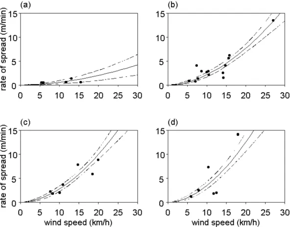
Predictions and 95% confidence bands for rate of spread as a function of wind speed, for fixed values of fuel height, are shown in Figure 3. Fuel heights shown are (a) 0.2 m, (b) 0.5 m, (c) 0.6 m and (d) 0.7m. Observations within ± 0.5 meters of these plot heights are shown in the figure.

Alternative spread rate model using bulk density as an independent variable The logarithmic form of the following model was fitted for each bulk density (<0.6 mm, <2.5 mm and total fuel)

[12] R = a Ub ρb

c

The best equation explained 74% of the variation in rate of spread - almost as good as was achieved using vegetation height - and was attained with the <2.5 mm bulk density (ranging from 1.6 to 7.8 kg m-3). Again spread rates at the higher wind speeds were underpredicted, and non-linear least squares was used to produce a better model. In this model estimates of a, b and c were 0.129 (s.e. = 0.063), 1.79 (s.e. = 0.17) and -1.67 (s.e. = 0.43), respectively. This model also had a mean absolute error of 1.0 m min-1.

Flame length

The procedures used to estimate the parameters in function [7] resulted in p = 0.0516 (s.e. 0.0126) and q = 0.453 (s.e. 0.038), accounting for 78% of the variation observed in flame length. Site effects were not significant after fitting the logarithmically transformed form of [7]. Flame length is plotted against Byram’s intensity in Figure 4, and the regression equation is shown (as a solid line).

A flame model of the form [7] requires estimates of the parameters involved in the calculation of fireline intensity: rate of spread, fuel consumed and heat of combustion. Fine fuel consumption in these experiments was basically estimated as a function of postburn diameters of

terminal stems, and 56% of the variation in this variable was explained by vegetation height (p<0.0001) and aerial dead fuel moisture content (p = 0.019), two variables that were selected by a stepwise regression. Since a precise evaluation of heat yield and fuel weight consumed by flaming combustion are infeasible under field conditions (Alexander 1982), simple estimates of heat yield and fuel consumption for use in the field are needed.

The results in Table 6 suggest that <2.5 mm aerial fuel loads in marginal fuel moisture conditions (site 1) and <6 mm aerial fuel loads otherwise (site 2), are acceptable surrogates for available fuel in mature EU-CT communities; equations are available to estimate these at the stand level from age (Fernandes and Rego 1996) or structure (Fernandes and Rego 1998a). Data from Vega et al. (1998a) for this vegetation type show a linear response of fine fuel reduction (ranging from nearly 100% to 80%) to dead fuel moisture (range 8-25%), and also a marked effect of live fuel moisture in spring burns; the low fuel consumption observed in site 3 is probably related to this live moisture effect, coupled to reduced flammability of the stand.

Standard values for heat yield are frequently suggested or assumed in the literature, e.g. 18,600 kJ kg-1 _{(Albini 1976). Heat yield of the shrub species in this study, after reducing the low}

heat content for the energy associated to water loss, can be assumed to vary within an interval of 20,500 to 21,000 kJ kg-1.

Discussion

Rate of fire spread in open fuel types has been shown to be mainly controlled by wind speed. This effect, as described by the exponent b of a power-law curve, extends in the literature from b = 0.4 (Trabaud 1979) to b = 2 (McArthur 1966). Linear or near-linear relationships between rate of spread and wind speed are reported in Arizona's chaparral (Lindenmuth and Davis 1973), gorse and heath in England (Thomas 1971) and Australian grassland (Cheney et al. 1993). In Tasmanian buttongrass moorland, Marsden-Smedley and Catchpole (1995) obtained b = 1.31, but the index decreased to 0.88 when two less reliable high intensity wildfires were excluded from the analysis. In the wind function of Rothermel (1972) the coefficient b is

parameterised in terms of the surface area-to-volume ratio (σ), and for this fuel type would range from 1.2 to 1.8, which corresponds to a fuel bed entirely made up of CT (σ = 43 cm-1) or EU (σ = 87 cm-1_{), respectively (Fernandes and Rego 1998b). In equation [11] b =1.83, which is closer}

to the higher value. Values of b = 1.1 or 1.2 are given by recent work in a variety of shrubland types, both in Europe (Fernandes 1998, Vega et al. 1998b) and Australasia (Catchpole et al. 1998a, McCaw 1998). Examination of plots of spread rate versus wind speed for fixed values of fuel height showed that the relationship was virtually linear above the lowest wind speed of 5 km h-1_{, as found by Cheney et al. (1998). Reflecting this linearity requires a more complicated}

model than the limited microplot data warrants, but this should be a consideration when producing a robust model for shrubland from a larger range of sites.

The coefficient c = 1.47, which in equation [11] describes the effect of vegetation height on rate of spread, seems large compared with those found in other shrubland studies. Trabaud (1979), Catchpole et al. (1998a), Vega et al. (1998b) and Fernandes (1998) obtained c = 0.35, 0.54, 0.66 and 0.84 respectively. Note that the effect of height is more reliably estimated in the data than the effects of wind speed or fuel moisture because the full range in fuel conditions for this vegetation type are represented in the microplots, whereas wind speed and aerial dead fuel moisture content only ranged from 5 to 27 km h-1 _{and 14 to 21%, respectively.}

The statistical analysis found no significant effect of species difference on fire spread rate despite the large differences in surface area to volume ratio, bulk density, loading and percentage of dead fuel. CT has higher fuel weight and dead to live ratio, while the relative amount of fuel in the <2.5 mm size class is greater in EU. Fuel particle properties of the two species are quite different: density is 0.32 g cm-3 for EU and 0.61 g cm-3 for CT, and surface area to volume ratio for the <2.5 mm class is 101 cm-1 and 47 cm-1 respectively (Fernandes and Rego 1998b). Lindenmuth and Davis (1973) and Cheney et al. (1993) found no effect of species difference (for species with very different surface area to volume ratio) on fire spread in chaparral and

grasslands, respectively. Catchpole et al. (1998b) also found no effect of surface area to volume ratio in laboratory experiments in fine fuels.

Over all sites cover only varied between 75% and 100%, whereas height ranged from 0.1m to 0.75m, and this may explain the lack of significance in cover. The percentages of the species varied from 0 to 100%, and the lack of significance indicates that species structural differences are not affecting fire spread rate. The percentage of fine dead fuel, which ranged from 25% to 90%, was surprisingly found to be non-significant, but this may reflect the unreliability of the visual estimation method used. Ocular estimates of dead fuel percentage and actual values resulting from destructive sampling were compared by Fernandes (1997) for both species, who found a reasonably good agreement for CT - whose dead foliage is very conspicuous - but inconsistent values for EU.

The results suggest that vegetation height is the most suitable fuel-complex parameter for inclusion in a fire spread model for this vegetation type. This variable, frequently used as a predictor of shrubland fire spread, has the advantage of being easily assessed on-site. Litter fuel beds have a roughly constant bulk density (e.g. Brown 1981). However, that is not the case in the CT-EU fuel type (Fernandes 1997), or in other elevated fuels (e.g. Rundel and Parsons 1979, Brown 1982, Armand et al. 1993), where bulk density decreases with increasing height. Thus the effect of height found in this analysis may well relate to the effect of change in bulk density. Because the effects of depth and load are combined in bulk density, we believe that preference should be given to this variable, as in the model for gorse and heather presented by Thomas (1971). This idea is supported by Fourty (1993), who analyzed data from laboratory burns in reproduced fuel beds of Quercus coccifera shrubs and concluded that rate of fire spread was controlled by bulk density for several combinations of fuel load and depth. Also, physionomically similar plant communities with the same vegetation depth may have quite different bulk densities, depending on the structure of the individual species of which they are composed. For example, the biomass of three low heathland communities in Northern Spain, dominated by Erica tetralix, E. umbellata and Ulex minor ranged from 2.7 to 23.6 t ha-1

respectively, but their heights merely varied between 0.60 and 0.69 m (Basanta et al. 1988). Therefore, bulk density can be more useful than fuel loading or depth when data from structurally similar fuels are combined with the purpose of developing a fire behaviour model for a broad vegetation type.

The use of bulk density under operational circumstances would obviously be more troublesome than the use of fuel height, because it would require an assessment of height plus vegetation cover and fuel load. Fernandes and Rego (1996) related bulk density to stand age, which poses the problem of estimating age itself. Reliable age information is probably restricted to areas with active prescribed burning programs. Finally, one has to consider the possibility of directly using age as a fire spread predictor, as in the model of Marsden-Smedley and Catchpole (1995) for buttongrass moorland, where age could easily be determined, and was used as a surrogate for the effects of fuel load and dead fuel load which could not be separated. Since fuel characteristics are strongly time-dependent in CT-EU stands, age seems a viable alternative, even if less attractive from the operational viewpoint because of the difficulties associated to its determination.

Shrubland fires are crown fires (Rothermel 1972), and this classification seems especially applicable when the vegetation is low and vertically continuous (Marsden-Smedley 1993), like in the present study. The existence of litter is not required for sustained fire propagation in the CT-EU fuel type, but from the analysis of fire spread in site 1 it appears that litter moisture has an effect on spread rate. Further research is required to clarify the role of both litter moisture and structure in shrubland fire behaviour.

Empirical flame models that, after Byram (1959), rely on a power function of fireline intensity generally indicate that flame length or height of a headfire is approximately proportional to the square root of intensity. This holds for the present study and has been verified in other heathland fuels (Marsden-Smedley and Catchpole 1995, Catchpole et al. 1998a, Vega et al. 1998b). Byram’s equation (shown as a dashed line in Figure 4) overpredicts flame lengths, but the equation was based on flame length from tip to mid-point of the base of the flame.

Equation [7], especially in its coefficient p = 0.0516 approaches the L = 0.0475I 0.493

relationship derived for a mixture of pine litter and shrubs by Nelson and Adkins (1986), who used flame streamlines as the reference to measure flame angle. (Nelson and Adkin’s equation is shown as a dotted line in Figure 4). Hence, this study's results do not support the reexamination of the flame length dependency on Byram's intensity that was proposed by Catchpole et al. (1993) following their flame length interpretation.

The adequacy of a microplot sampling methodology to model fire behaviour is influenced by the magnitude of rate of fire spread and intensity. Fire behaviour could be measured near the microplots and data collection was more concentrated when the fires were burning slower and with shorter flames. Increased smoke production and higher heat release during periods of more severe fire behaviour affected visibility and compelled the observers to stand off from the microplots, thus reducing measurement accuracy. Video recording partially overcame those problems, but it is clear, as Smith et al. (1993) stated, that techniques to remotely measure fire behaviour parameters would be preferable in a microplot study, such as flame sensors (e.g. Finney and Martin 1992) and thermocouples or electronic timers to determine fire arrival and departure times in a microplot. The confidence bands in Figure 3 show that the reliability of the prediction equation [11] is less at higher spread rates because of the increased variability. Note also that only microplots from site 2 have spread rates above 5 m min-1.

Microplot size can also play an important role in the quality of data. In the CT-EU fuel type 1 m2 _{microplots are adequate to select patches of roughly constant vegetation height when the}

ground cover is total, or nearly total. Larger observation units would consequently result in more heterogeneous fuel conditions within a microplot and in microplots with similar average fuel characteristics. Nevertheless, fire behaviour measurement would be easier in bigger microplots, and less prone to experimental error during fast spread periods. More robust relationships between rate of spread and wind speed could also be derived using larger microplot areas, since

fire behaviour is not modified instantaneously by an alteration in wind speed (e.g. Sneeuwjagt and Frandsen 1977). On the other hand, the smallness of the plots tends to reduce the chance for a wind change in direction or velocity. Therefore, the microplot size needs to be chosen according to the fuel type involved and the primary objective(s) of the experiment. E.g., taller shrubland would require larger microplots, and an experiment designed to study pine litter reduction or flame residence time could benefit from smaller microplots. Preliminar tests should be conducted to help in defining the ideal size.

Flame depth in a given fuel type increases with the fire spread rate. It can therefore be argued that a microplot may be too small in relation to the depth of the flame, implying that fire behaviour is being influenced by fuels outside the microplot. However, and since the microplots have been established in areas where the fuel-complex is reasonably uniform, significant fuel differences between the microplot and its immediate vicinity are unlikely to occur.

Only a few microplots were occupied by a single species in this study, since shrubs of both species alternate at a very small spatial scale in this vegetation type. A microplot approach to quantify the influence of fuel characteristics on fire behaviour will presumably yield the best results if the microplots are established in patches of individual species or fuel types that alternate spatially on a larger scale.

Conclusion

Spatial variability of fuels and temporal variability of wind induced relatively large ranges of variation in fire behaviour within a single burn. This study showed that minor changes which occur within a fuel type affect fire behaviour and can be empirically modelled in the frame of a microplot experimental design. However, the experimental measurements taken, and the correlation among variables, precluded the isolation of the individual influence of fuel geometry variables on rate of fire spread. The most significant structural descriptor of the CT-EU fuel-complex for determining spread rate was fuel height, although some basis exists for preferring bulk density as a predictor variable.

Microplot sampling can be used in field studies on fire behaviour, but the usefulness and validity of the results will strongly depend on adequate experimental procedures. The data collection process should rely on techniques capable of providing precise and complete measurements of the involved variables.

The methods usually used to test and develop fire behaviour models can be applied to sets of individual small plots within burns. A microplot approach can be used to complement the results obtained in traditional fire behaviour experiments, and - if scale problems are not a concern - can be used as a stand-alone procedure. Important and unsolved research questions, such as the effect of high wind speeds on fire propagation, the role of live fuel moisture or the definition of thresholds for sustained fire spread could greatly benefit from a microplot approach.

Acknowledgments

This study was partially funded by the European Comission under contract EV5V-CT94-0473 and by a grant (PRAXIS XXI/BM/2015/94) from Junta Nacional de Investigação Científica e Tecnológica. The authors are grateful to the personnel at the Forestry Department of UTAD who participated in the field work. Two anonymous reviewers provided helpful suggestions.

References

Agroconsultores-COBA. 1991. Carta de solos do Nordeste de Portugal. UTAD.

Albini, F.A. 1976. Estimating wildfire behavior and effects. USDA For. Serv. Gen. Tech. Rep. INT-30. Alexander, M.E. 1982. Calculating and interpreting forest fire intensities. Can. J. Bot. 60: 349-357. Andrews, P.L. 1980. Testing the fire behavior model. In Proceedings of the 6th Conf. on Fire and Forest

Meteorology, 22-24 April 1980, Seattle, Washington. Edited by Society of American Forests, Washington D.C. pp. 70-77.

Armand, D., Etienne, M., Legrand, C., Marechal, J., and Valette, J.C. 1993. Phytovolume, phytomasse et relations structurales chez quelques arbustes méditerranéens. Ann. Sci. Forest. 50: 79-89.

Basanta, M., Vizcaíno, E., and Casal, M. 1988. Structure of shrubland communities in Galicia (NW Spain). In Diversity and pattern in plant communities. SPB Academic Publishing, The Hague, The Netherlands. pp. 25-36.

Brown, J.K. 1981. Bulk densities of nonuniform surface fuels and their application to fire modeling. Forest Sci. 27(4): 667-683.

Brown, J.K. 1982. Fuel and fire behavior prediction in big sagebrush. USDA For. Serv. Res. Pap. INT-290.

Byram, G.M. 1959. Combustion of forest fuels. In Forest Fire Control and Use. McGraw-Hill Book Company, New York. pp. 61-89.

Catchpole, E.A., Hatton, T.J., and Catchpole, W.R. 1989. Fire spread through nonhomogeneous fuel modelled as a Markov process. Ecol. Model. 48: 101-112.

Catchpole, E.A., Catchpole, W.R., and Rothermel, R.C. 1993. Fire behavior experiments in mixed fuel complexes. Int. J. Wildland Fire 3(1): 45-57.

Catchpole, W., Bradstock, R., Choate, J., Fogarty, L., Gellie, N., McCarthy, G., McCaw, L., Marsden-Smedley, J., and Pearce, G. 1998a. Cooperative development of equations for heathland fire behaviour. In Proceedings of the 3rd International Conf. on Forest Fire Research & 14th Fire and Forest Meteorology Conf., 16-20 Nov. 1998, Luso. Edited by D.X. Viegas. ADAI, University of Coimbra, Portugal. pp. 631-645.

Catchpole, W.R, Catchpole, E.A., Rothermel, R.C., Morris, G.A, Butler, B.W., and Latham, D.J. 1998b. Rate of spread of free-burning fires in woody fuels in a wind tunnel. Combust. Sci. Technol. 131: 1-37.

Cheney, N.P. and Gould, J.S. 1997. Fire growth and acceleration. Int. J. Wildland Fire 7(1): 1-5.

Cheney, N.P., Gould, J.S., and Catchpole, W.R. 1993. The influence of fuel, weather and fire shape variables on fire-spread in grasslands. Int. J. Wildland Fire 3(1): 31-44.

Cheney, N.P., Gould, J.S., and Catchpole, W.R. 1998. Prediction of fire spread in grasslands. Int. J. Wildland Fire 8(1): 1-13.

Fernandes, P.M. 1997. Caracterização do combustível e do comportamento do fogo em comunidades arbustivas do Norte de Portugal. Unpublished MSc. Thesis, UTAD.

Fernandes, P.M. 1998. Rate of fire spread modelling in Portuguese shrubland. In Proceedings of the 3rd International Conf. on Forest Fire Research & 14th Fire and Forest Meteorology Conf., 16-20 Nov. 1998, Luso. Edited by D.X. Viegas. ADAI, University of Coimbra, Portugal. pp. 611-628.

Fernandes, P. and Rego, F.C. 1996. Changes in fuel structure and fire behaviour with heathland aging in Northern Portugal. To appear In the Proceedings of the 13th Conf. on Fire and Forest Meteorology, Oct. 1996, Lorne, Melbourne, Australia.

Fernandes, P.M., and Rego, F.C. 1998a. Equations for estimating fuel load in shrub communities dominated by Chamaespartium tridentatum and Erica umbellata. In Proceedings of the 3rd International Conf. on Forest Fire Research & 14th Fire and Forest Meteorology Conf., 16-20 Nov. 1998, Luso. Edited by D.X. Viegas. ADAI, University of Coimbra, Portugal. pp. 2553-2564. Fernandes, P. and Rego, F.C. 1998b. A new method to estimate fuel surface area-to-volume ratio using

Finney, M.A., and Martin, R.E. 1992. Calibration and field testing of passive flame height sensors. Int. J. Wildland Fire 2(3): 115-122.

Forestry Canada Fire Danger Group. 1992. Development and structure of the Canadian forest fire behavior prediction system. Forestry Canada, Information Report ST-X-3.

Fourty, T. 1993. Comportement du feu dans Quercus coccifera: analyse en composantes principales. INRA, Doc. PIF9303.

Frandsen, W.H., and Andrews, P.L. 1979. Fire behavior in nonuniform fuels. USDA For. Serv. Res. Pap. INT-232.

Fujioka, F.M. 1985. Estimating wildland fire rate of spread in a spatially nonuniform environment. Forest Sci. 11(1): 21-29.

Gill, A.M. and Moore, P.H. 1994. Some ecological research perspectives on the disastrous Sydney fires of January 1994. In Proceedings of the 2nd Int. Conf. on Forest Fire Research, Nov. 1994, Coimbra. Edited by D.X. Viegas. ADAI, University of Coimbra, Portugal. Pp. 63-72.

Gomes, J.M. 1982. Avaliação de combustíveis arbustivos do sub-bosque de povoamentos de Pinus

pinaster Ait. Relat. de estágio, IUTAD.

Hawkes, B.C. 1986. Micro-plot approach to prescribed fire effects research. In Proceedings of the Symposium Prescribed Burning in the Midwest: State of the Art., 3-6 March 1986, Stevens Point, Wisconsin. pp. 45-53.

Hunt, S.M., and Crock, M.J. 1987. Fire behaviour modelling in exotic pine plantations: testing the Queensland Department of Forestry "Prescribed Burning Guide Mk III". Aust. Forest. Sci. 17: 179-189.

Lindenmuth, A.W., and Davis, J.R. 1973. Predicting fire spread in Arizona's oak chaparral. USDA For. Serv. Res. Paper RM-101.

Marsden-Smedley, J.B. 1993. Fuel characteristics and fire behaviour in Tasmanian buttongrass moorlands. Parks and Wildlife Service, Dept. of Environment and Land Management, Hobart, Australia.

Marsden-Smedley, J.B., and Catchpole, W.R. 1995. Fire behaviour modelling in Tasmanian buttongrass moorlands. II. Fire behaviour. Int. J. Wildland Fire 5(4): 215-228.

McAlpine, R.S., and Wakimoto, R.W. 1991. The acceleration of fire from point source to equilibrium spread. Forest Sci. 37(5): 1314-1337.

McArthur, A.G. 1966. Weather and grassland fire behaviour. Forest Research Institute, Forestry and Timber Bureau, ACT, Australia.

McCaw, L. 1998. Research as a basis for fire management in mallee-heath shrublands of Southwestern Australia. In Proceedings of the 3rd International Conf. on Forest Fire Research & 14th Fire and Forest Meteorology Conf., 16-20 Nov. 1998, Luso. Edited by D.X. Viegas. ADAI, University of Coimbra, Portugal. pp. 2335-2348.

Nelson, R.M., and Adkins, C.W. 1986. Flame characteristics of wind-driven surface fires. Can. J. Forest Res. 16: 1293-1300.

Nelson, R.M. and C.W. Adkins. 1988. A dimensionless correlation for the spread of wind-driven fires. Can. J. Forest Res. 18: 391-397.

Rivas-Martinez, S. 1979. Brezales y jarales de Europa Occidental. Lazaroa 1: 5-128.

Rothermel, R.C. 1972. A mathematical model for predicting fire spread in wildland fuels. USDA For. Serv. Res. Pap. INT-115.

Rundel, P.W., and Parsons, D.J. 1979. Structural changes in chamise (Adenostoma fasciculatum) along a fire-induced age gradient. J. Range Manage. 32(6): 462-466.

Ryan, K.C., and Noste, N.V. 1985. Evaluating prescribed fires. In Proceedings of the Symposium and Workshop on Wilderness Fire, 15-18 Nov., 1983, Missoula, Montana.. USDA For. Serv. Gen. Tech. Rep. INT-182. pp. 230-238

Simard, A.J., Eenigenburg, J.E., Adams, K.B., Nissen, Jr., R.L., and Deacon, A.G. 1984. A general procedure for sampling and analyzing wildland fire spread. Forest Sci. 30: 51-64.

Smith, J.K, Laven, R.D., and Omi, P.N. 1993. Microplot sampling of fire behavior on Populus

tremuloides stands in North-Central Colorado. Int. J. Wildland Fire 3(2): 85-94.

Sneeuwjagt, R.J., and Frandsen, W.H. 1977. Behaviour of experimental grass fire versus predictions based on Rothermel's fire model. Can. J. Forest Res. 7: 357-367.

Snowdon, P. 1991. A ratio estimator for bias correction in logarithmic regressions. Can. J. Forest Res. 21: 720-724.

Thomas, P.H. 1971. Rates of spread of some wind-driven fires. Forestry 44: 155-175.

Trabaud, L. 1979. Etude du comportement du feu dans la garrigue de chêne kermes à partir des températures et des vitesses de propagation. Ann. Sci. Forest. 36: 13-35.

Valette, J.C., Vega, J., Botelho, H., Gillon, D., Hernando, C., and Ventura, J. 1996. Forest fire prevention through prescribed burning: prediction of effects on trees. To appear In the Proceedings of the 13th Conf. on Fire and Forest Meteorology, Oct. 1996, Lorne, Melbourne, Australia.

Vega, J.A, Cuiñas, P., Fonturbel, M. and Fernández, C. 1998a. Planificar la prescripción para reducir combustibles y disminuir el impacto sobre el suelo en las quemas prescritas. To appear In Taller sobre Empleo de Quemas Prescritas para Prevención de Incendios Forestales, 10-13 Nov. 1998, Lourizán. Sociedade Española de Ciencias Forestales.

Vega, J.A., Cuiñas, P., Fontúrbel, T., Pérez-Gorostiaga, P., and Fernández, C. 1998b. Predicting fire behaviour in Galician (NW Spain) shrubland fuel complexes. In Proceedings of the 3rd International Conf. on Forest Fire Research & 14th Fire and Forest Meteorology Conf., 16-20 Nov. 1998, Luso. Edited by D.X. Viegas. ADAI, University of Coimbra, Portugal. pp. 713-728.

Viegas, D.X., Viegas, M.T., and Ferreira, A.D. 1992. Moisture content of fine forest fuels and fire occurrence in Central Portugal. Int. J. Wildland Fire 2(2): 69-86.

Table 1. Pre-burn fuel variables measured in the microplots.

H cov ved

Plot CT EU overall CT EU total CT EU overall Site 1 average 0.51a 0.49a 0.53a 29a 68a 97a 75a 37a 49a

(n=22) min. 0.10 0.35 0.42 0 10 80 70 20 20 max. 0.73 0.72 0.70 95 100 100 100 75 80 Site 2 average 0.57a 0.56a 0.57a 46a 47b 94a 84b 30b 57a

(n=25) min. 0.42 0.40 0.41 0 3 80 80 15 28

max. 0.81 0.80 0.81 95 90 100 90 50 87 Site 3 average 0.19b 0.25b 0.20b 78b 15c 93a 70c 25ab 62a

(n=10) min. 0.10 0.25 0.10 25 0 75 70 25 32 max. 0.30 0.25 0.30 100 75 100 70 25 70 Note: H = height, m; cov = ground cover %; ved = visually estimated fine dead fuel %.

Within a column, mean values followed by the same letter are not different at the 5% significance level, according to the Tukey-Kramer HSD test.

Table 2. Pre-burn fuel loads (kg m-2_{) by live and dead size classes estimated for the microplots.}

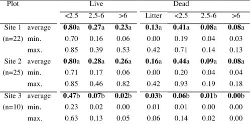
Plot Live Dead

<2.5 2.5-6 >6 Litter <2.5 2.5-6 >6 Site 1 average 0.80a 0.27a 0.23a 0.13a 0.41a 0.08a 0.08a

(n=22) min. 0.70 0.16 0.06 0.00 0.19 0.04 0.03 max. 0.85 0.39 0.53 0.42 0.71 0.14 0.13 Site 2 average 0.80a 0.28a 0.26a 0.16a 0.44a 0.09a 0.08a

(n=25) min. 0.71 0.17 0.06 0.00 0.20 0.04 0.04 max. 0.85 0.46 0.82 0.42 0.93 0.19 0.18 Site 3 average 0.47b 0.07b 0.02b 0.03b 0.06b 0.01b 0.00b

(n=10) min. 0.23 0.02 0.00 0.01 0.01 0.00 0.00 max. 0.63 0.13 0.05 0.06 0.14 0.02 0.00

Within a column, mean values followed by the same letter are not different at the 5% significance level, according to the Tukey-Kramer HSD test.

Table 3. Weather conditions during the burns. Plot Burn date and

ignition time Days since rain T, o_C RH, % U, km h-1 Site 1 16 Nov 1994, 16:00 3 14 55 8.9 (5.5-14.5) Site 2 16 Jan 1995, 14:30 7 15 40 14.5 (7.4-27.0) Site 3 24 March 1995, 12:00 5 12 51 9.5 (5.4-15.5)

Note: T = air temperature; RH = air relative humidity; U = 2 m windspeed (mean and range in the microplots, n=22 for site 1, n=25 for site 2 and n=10 for site 3).

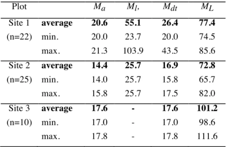
Table 4. Fine fuel moisture contents (%) in the microplots.

Plot Ma Ml, Mdt ML Site 1 average 20.6 55.1 26.4 77.4 (n=22) min. 20.0 23.7 20.0 74.5 max. 21.3 103.9 43.5 85.6 Site 2 average 14.4 25.7 16.9 72.8 (n=25) min. 14.0 25.7 15.8 65.7 max. 15.8 25.7 17.5 82.0 Site 3 average 17.6 - 17.6 101.2 (n=10) min. 17.0 - 17.0 98.6 max. 17.8 - 17.8 111.6

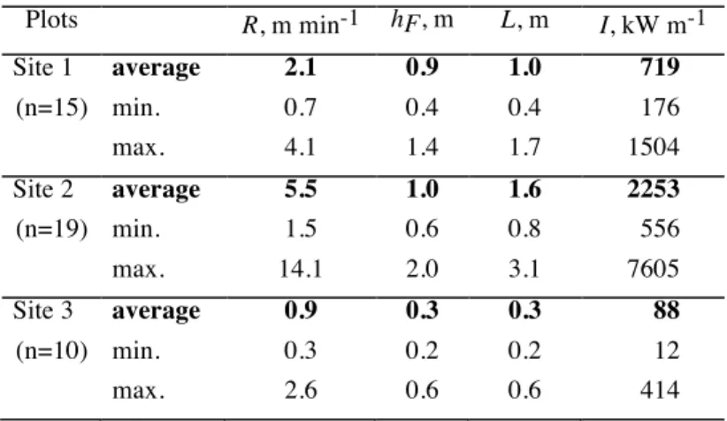
Table 5. Fire behaviour descriptors in the microplots. Plots _{R, m min}-1 _{hF, m L, m I, kW m}-1 Site 1 average 2.1 0.9 1.0 719 (n=15) min. 0.7 0.4 0.4 176 max. 4.1 1.4 1.7 1504 Site 2 average 5.5 1.0 1.6 2253 (n=19) min. 1.5 0.6 0.8 556 max. 14.1 2.0 3.1 7605 Site 3 average 0.9 0.3 0.3 88 (n=10) min. 0.3 0.2 0.2 12 max. 2.6 0.6 0.6 414

Note: R = rate of spread; hF = flame height; L = flame length; I = fireline intensity.

Table 6. Fuel consumption descriptors in the microplots.

Plots C, % _{dt, mm} w 2.5 % w, % Site 1 average 2 2.8 91 72 (n=15) min. 0 2.0 72 53 max. 10 4.5 100 88 Site 2 average 0 3.9 100 85 (n=19) min. 0 2.5 100 71 max. 0 6.0 100 100 Site 3 average 3 1.4 27 23 (n=10) min. 0 1.0 18 16 max. 10 2.0 40 35

Note: C = post-burn cover; dt = average terminal twig and stem diameter; w 2.5 = fuel reduction in the <2.5 mm size class as a % of its preburn load; w = fine fuel (<6 mm) consumption as a % of its preburn load.

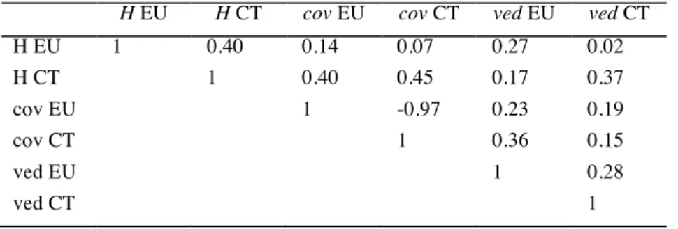
Table 7. Within-site correlation coefficients of measured fuel variables for sites 2 and 3. H EU H CT cov EU cov CT ved EU ved CT

H EU 1 0.40 0.14 0.07 0.27 0.02 H CT 1 0.40 0.45 0.17 0.37 cov EU 1 -0.97 0.23 0.19 cov CT 1 0.36 0.15 ved EU 1 0.28 ved CT 1

Figure 1. Residuals of ln(spread rate) after fitting ln(wind speed) and ln(height) to the three sites (equation [9]) plotted against average dead fuel moisture content for site 1 (crossed circles), site 2 (open circles), and site 3 (triangles).

Figure 2. Predicted values versus observed values from equation [11] for site 1 (crossed circles), site 2 (open circles), and site 3 (triangles).

Figure 3. Predictions (unbroken lines) and 95% confidence bands (dashed lines) for rate of spread as a function of wind speed, for fixed values of fuel height. Fuel heights shown are (a) 0.2 m, (b) 0.5 m, (c) 0.6 m and (d) 0.7m. Observations within ± 0.5 meters of these plot heights are shown.

Figure 4. Flame length versus Byram’s intensity: regression equation [7] shown as solid line with 95% confidence bands shown as vertical lines, Byram’s equation shown as dashed line, and equation from Nelson and Adkins (1986) shown as dotted line.