Land reform with human capital: A new analysis using the theory of economic growth and the theory of the firm

UNIVERSIDADE DE ÉVORA

DEPARTAMENTO DE ECONOMIA

DOCUMENTO DE TRABALHO Nº 2005/13

July

Land reform with human capital: A new analysis using

the theory of economic growth and the theory of the firm

Miguel Rocha de Sousa

*

Universidade de Évora, Departamento de Economia

* _{I greatly acknowledge many suggestions from my supervisor Abel Mateus, António Antunes, Adão}

Carvalho, Cesaltina Pires, Leonor Carvalho and Pedro Henriques. This paper was presented at the 3rd

International Conference on European and International Political and Economic Affairs, 26-28th _{May 2005}

at ATINER Institute, Athens, Greece. I thank participants for helpful suggestions. Any remaining errors are my own. I thank Fundação Eugénio de Almeida at Évora for financial support through a PhD scholarship.

UNIVERSIDADE DE ÉVORA

DEPARTAMENTO DE ECONOMIA

Largo dos Colegiais, 2 – 7000-803 Évora – Portugal

Tel.: +351 266 740 894 Fax: +351 266 742 494

www.decon.uevora.pt

wp.economia@uevora.pt

Abstract:

In section 1 we refer to a historical synopsis, section 2 classifies the different land reforms using

KAWAGOE (1999) typology. Afterwards we link the concepts of human capital and land reform within the

theory of economic growth.

In section 3 a simplified formal dynamic model of land reform based on the neoclassical theory of economic

growth is introduced, following SOLOW-SWAN models. In section 4 an endogenous growth model tries to

evaluate land reform in the process of economic growth, based on the ROMER (1990) model. We further

try to relate the notion of convergence with successful land reform.

The main conclusion of these sections is that with the neoclassical exogenous framework there is

convergence between small landholders and latifundia holders. This is a successful land reform: there is a

finite time horizon that allows almost landless illiterate to catch up with rich literate farmers. In the case of

endogenous growth there is never convergence thus the land reform process fails.

Another conclusion in the endogenous framework is that, by reverse causality, failed land reforms result

from perpetuating initial differential human capital stocks.

In section 5, another approach is to extend ARROW (1962) learn by doing model to evaluate land reform

as a structural break (or cut-off point). A condition for land reform viability is established, creating a

Possibility Set of Recovery of Human Capital (PSRHC).

In section 6 we simplify the theory of the firm JOVANOVIC´s (1982) model, applying it to agricultural firms

to explain birth, life and death of latifundia. We establish the date and process of land reform, as a cut-off

process, in which it arises from the failure of firms.

Finally, in section 7, we conclude and present in section 8 the references.

Keywords:

Land reform, human capital, growth theory

JEL Classification:

Q15,

O0

INDEX

1. Introduction

2. Typologies of land reform and static analysis 3. Neoclassical growth

4. Endogenous growth 5. Arrow’s LBD

6. Jovanovic’s theory of firm 7. Conclusion

1. Introduction

This paper analyses the process of land reform, in the second section some typologies of land reform and a static model of land reform is presented, in section 3 the model of neoclassical growth is analysed for land reform, in section 4, the new theory of endogenous growth is scrutinised for land reform, section 5 presents ARROW’s learn by doing process applied to land reform, section 6 does the same for the JOVANOVIC’s firm model applying it to land reform, finally section 7 concludes and section 8 presents the references.

ROCHA DE SOUSA (2005a,b) presents a detailed historical analysis of the land reform processes and presents tables 2 to 5 in his annex to synthesize it. For an empirical analysis of land reform efficiency evaluation see ROCHA DE SOUSA et al. (2004).

2. Typologies of land reform and static analysis

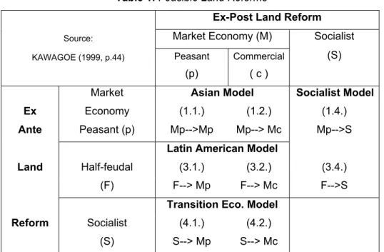
ROCHA DE SOUSA (2005a,b) presents first all the theoretical land reforms a 4X4 matrix, but then realizes that in the real world there are only 3X3 feasible land reforms:

Table 1: Feasible Land Reforms

Ex-Post Land Reform

Source: Market Economy (M) Socialist

KAWAGOE (1999, p.44) Peasant Commercial (S)

(p) ( c )

Market Asian Model Socialist Model

Ex Economy (1.1.) (1.2.) (1.4.)

Ante Peasant (p) Mp-->Mp Mp--> Mc Mp-->S

Latin American Model

Land Half-feudal (3.1.) (3.2.) (3.4.) (F) F--> Mp F--> Mc F-->S

Transition Eco. Model

Reform Socialist (4.1.) (4.2.)

(S) S--> Mp S--> Mc

ROCHA DE SOUSA (2005b) presents two static human capital models for land reform. Here we present the second model in which we have two trade-off effects.

We consider the variable human capital (H) as a state variable which influences output (Y) and we do analyse in a broader context of start-up cost what happens in terms of efficiency analysis with the introduction of labour (L).

Hypotheses:

i) model with 2 factors: H, human capital and L labour.

ii)

_H

B

_>

_H

S_{: the level of (initial) human capital from latifundia landholders (B-big) is greater than the smaller}

landholders (S) – this is our version of start-up cost.

iii) The fundamental hypothesis is that the additional human capital (investment in human capital) increases labour productivity, which means that the crossed derivative has a positive sign:

(

)

2

0

Y

Y

_L

L H

H

∂

∂

∂

₌

∂

_>

∂ ∂

∂

.

Thus, the profit function now is:

( )

L

p Y H L Y H L

( ( , )). ( , )

w L

.

π

=

−

In this profit function specification, in which H is just a state variable and not a decision variable, producers adjust L as decision variable.

2.1. Static Model of big landholding

We have a rather simple hypothesis which is the fact that the human capital from the big landholder is greater than the human capital of the smaller landholder (“minifundia”):

_H

B

_>

_H

S_.

Thus we will solve the problem of the big landholder (latifundia):

.

.

.

0

d

p

Y

Y

Y

p

w

dL

Y

L

L

π

₌

∂ ∂

₊

∂

_{− =}

∂

∂

∂

So, solving as it is usual, in the neoclassical literature, for the monopolist we end up with:

,

1

Y p

w

p

Y L

p

ε

−

∂ ∂ =

As by hypothesis iii)

Y

L

∂

∂

is increasing on H, then

Y

w

L

∂

∂

(which is the marginal cost of this model) is decreasing on H, which implies that the big firm has a lower marginal cost (than the perfect competition ones).

2.2. Static Model of small firm

For the small firm the profit maximization yields immediately, price equal to marginal cost:

w

p

Y L

=

∂ ∂

.

2.3. Comparative statics

Thus, comparing section 2.1. of the big firm with section 2.2. of the small firm, we can do a very illustrative welfare analysis, even though in a static context and in partial equilibrium.

We have two opposite side effects in the Land Reform (LR) evaluation setting:

Effect A) The pro-efficiency effect resulting from the change from monopoly to perfect competition1_;

Effect B) The pro-learning effect of labour marginal cost reduction due to the change from small minifundia to big

farmers due to an increase in human capital.

If A>B then LR is a viable policy because the efficiency gain compensates the loss due to human capital (increase in marginal cost due to the reduction of human capital)

If A<B then LR is a non-viable policy because the efficiency gain does not compensate the loss in human capital (increase in marginal cost due to a reduction in H).

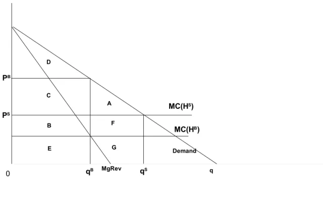
Let us see graphically with the hypothesis of a constant marginal cost (linear and constant w, just a function of H) and without loss of generality2_:

1 _{The paper assumes that when the land reform takes place, the “latifundia” (regional monopolist) is divided and the}

resulting market structure is one of perfect competition. This assumption is crucial to our results and should be taken into account.

0 q A B MC(HS₎ MC(HB₎ Demand MgRev C D E F G qB _qS PS PB

Figure 1: Welfare analysis of Land Reform

In this Figure 1 we can observe the following:

Monopolist (One Big firm B) Perfect Competition (N Small firms S)

Consumer Surplus = D Producer Surplus = C+B Total Surplus = D+C+B

Consumer Surplus = D+C+A Producer Surplus = 0 Total Surplus = D+C+A Comparison of total surplus:

i) Viable Land Reform:

Perfect Competition Net Total Surplus>Monopoly Net Total Surplus [A>B] ii) Non-Viable Land Reform:

Perfect Competition Net Total Surplus<Monopoly Net Total Surplus [A<B]

Thus summing up, the policy of land reform in this setting of broader start-up cost is only viable if the pro-efficiency effect dominates the pro-learning effect, even in static terms.

3. Neoclassical growth and land reform

This section and the next one follows ROCHA DE SOUSA (2005d), in which more detail is used for the derivation of the results.

The model used is the standard neoclassical growth model as in BARRO and SALA-I-MARTIN (1995) with human capital. We assume the usual INADA conditions and the law of motion of the human capital intensity per unit of land are standard3_{. The new idea is to apply economic growth models to a land reform setting.}

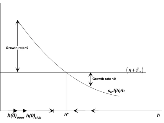
The figure 2 analyses a standard SOLOW-SWAN model in which we assume that a successful land reform program would yield the same final steady state for human capital intensity per unit of land (H/L).

3 _{The law of motion of human capital intensity per unit of land (h=H/L) is:}

₍

₎

h n h f s h•= _H. ( )− +δ_H . , where sH stands

for saving rate, f(h) the production function, n the growth rate of population,

δ

_H is the depreciation rate of human capital. The steady state is obtained by h•=0.

h h* sH.f(h)/h

(

n

+

δ

H

)

Growth rate>0 Growth rate <0 h(0)rich h(0)_poor

Figure 2 – Dynamics of SOLOW-SWAN model with successful Land Reform

Next we present the same figure but instead we argue that the savings function in the steady state can be different between rich and poor economies.

h

h*

rich sHrich.f(h)/h

(

n

+

δ

H

)

Growth rate>0 Growth rate >0 h(0)_rich h(0)_poor sHpoor.f(h)/h

h*

poor

Figure 3- Conditional convergence in SOLOW-SWAN and failure of Land Reform

At the steady state h* in figure 2 we have accomplished full land reform, because after having started from different initial human capital-land average ratios (higher productivity from initial latifundia holders) we arrive at the same human capital land ratios for both types of agents.

If we start from different initial human capital land holdings ratios and with different (human capital) savings preferences there might be divergence and not convergence. The steady state for the rich (with higher savings) might be higher, and even after having started from an higher human capital per unit of land (for the rich) their growth rates in the transition to the equilibrium might be proportionally higher than the poor.

Then this would be a case of failed land reform, because the poor never catch with the rich – instead of what we had seen in Figure 2 – where there was successful land reform we have dismal land reform – see Figure 3. The important issue is the time it takes the poor less endowed to catch up with the richer human capital endowed ones. Does it take more than one generation to arrive to the steady state?

MANKIW, ROMER and WEIL (1992) present a three sector model with labour, physical and human capital. Our version is even simpler and nevertheless tries to depict what happens in a land reform SOLOW-SWAN setting only with land and human capital.

4. Endogenous growth and land reform

4.1. The model

This section follows ROCHA DE SOUSA (2005d) using ROMER’s model (1990).

We adapted it to the land reform setting. In stead of having only physical capital and two types of labour (non-specialized and (non-specialized – human capital) we keep the distinction between the two types of labour, physical capital and we introduce the role of land. For a simplified exposition of ROMER’s model we follow Jones’s (1998, chapter 5) book.

The aggregate production function for our adapted model would thus be: (1)

Y

=

K

α

.

(

A

.

L

_Y

)

1−α

where, Y is agricultural output, K, means physical capital, A stands for the stock of ideas (endogenous to the model – as opposed to the SOLOW SWAN version in which A is exogenous) and LY is labour (non-specialized).

For a given level of technology A the production function in equation (1) exhibits constant returns to scale (CRS) in K and LY. Nevertheless when we recognise the role of the stock of ideas A, then there are increasing returns to scale.

That is if you double the stock of land, (non-specialized) labour and the stock of ideas then production (Y) will more than double.

If Ld means land or the size of the exploration (in ha) and we divide all (1) by Ld we end up with the production

function in the intensive form per unit of land – as we did in our SOLOW SWAN adapted model: (2)

y

=

k

α

.

(

A

.

l

_Y

)

1−α

where k stands for physical capital per unit of land, and lY stands for labour per unit of land.

The equations of motion for land and labour are the same as in the SOLOW model. Thus, land grows at the rate of n1:

(3) L•_d L_d =n₁

So, (total) labour growths at the growth rate of the population (n2):

(4)

L

•

L

=

n

₂

And besides all labour equals skilled labour (human capital) LA plus unskilled labour LY :

(5) L_A+L_Y =L

If we divide (5) by total land used we end up with labour intensity per unit of land: (6) l_A +l_Y =l

By some manipulations we have (as in our previous SOLOW SWAN model) the law of motion of the intensity of physical capital per unit of land (k):

(7) = −

(

+

δ

)

• 1 .y n s k k k .

Notice that this is the usual law of motion of physical capital as in the standard SOLOW SWAN model, but as we adapted it we have the variables per unit of land (and not in per capita terms).

Next we introduce the rate of growth of technical progress as in the ROMER model (as presented by JONES (1998, p.92-3)):

(8)

A

•

=

δ

.

L

_A

The equation presents A as the stock of knowledge, and

δ

is the growth rate of technical progress.

We might depict the evolution of this rate of growth

δ

depending on two factors: i)

δ

is increasing on A (because it depends on inventions such as Calculus, which increase productivity); and ii) it decreases with A because it is always more difficult to discover new things after having made a discovery (thus the productivity decreases).

So, our equation to sum up these two facts (i) and ii)): (9)

δ

=

δ

.Aφ

Replacing (9) in (8) we end up with: (10)

A

•

=

δ

.

A

φ

.

L

_A

Nevertheless, the most general case we could use a weight to consider the number of researchers (LA): (11)

φ λ

δ

L

A

A

•

=

.

_A

.

and we impose as JONES considers a restriction:

φ

<

1

.

This equation (11) shows up the fact that individual effort in research brings only small increases in output – that is there are constant returns to scale (CRS) at the individual level, but for the aggregate of the economy there are increasing returns to scale (IRS) due to externalities.

4.2. Growth in the Romer Model

Along a balanced growth path the output per unit of land (y), capital per unit of land (k) and the stock of ideas (A) must all grow at the same rate. Lower case letters denote per unit of land growth rates:

(12)

g

_y

=

g

_k

=

g

_A.

Do notice as JONES(1998) stresses that if there is no technological progress (gA=0), then there is no growth per unit

of land.

JONES asks himself the essential question: “What is the rate of technical progress along a balanced growth path?” This is a function of equation (11), the production function of ideas.

Here we follow again JONES (1998) to get this rate.

First we divide (11) by A and we get the following rate of innovation:

(13) _φ λ

δ

₋ • = . ₁ A L A A _A

Thus if along a balanced growth path we must have:

(14) g_A

A

A =• , as a constant.

So, equating (13) to (14), and by taking logs and derivatives on both sides of (13) we end up with: (15)

0

=

ln(

•

δ

)

+

λ

.

ln(

•

L

_A

)

−

(

1

−

φ

).

ln(

•

A

)

Noticing the time derivatives of logs as growth rates we end up with: (16) • • − = A A L L A A _{(1 ).} .

φ

λ

By (14) g_A A A =• , and as

L

A

L

_A

=

L

L

=

n

₂ • •

(because the number of researchers must grow at most as the population4_{) so we solve it in order to gA and obtain the central equation which yields endogenous growth:}

(17)

φ

λ

−

=

1

.

n

₂

g

_A .

Thus the long run growth of the economy is given by the ideas’ production function parameters

λ

, and

1

−

φ

, and by the growth rate of researchers (=growth rate of population = n2). In this model, as opposed to the conventional

SOLOW SWAN model, population growth (n2) brings more economic growth. Special cases:

CASE 1

λ

=

1

;

φ

=

0

.

This immediately implies by equation (11) gA=n2. That is the balanced growth path depends only on the population

growth rate (n2). Thus the productivity of researchers becomes a constant:

(18)

A

•

=

δ

.

L

_A

In this special case (18) JONES (1998) states that there is no duplication effort and the productivity of a researcher is independent of the stock of ideas discovered in the past.

If the number of researchers is constant (LA) then this economy creates each period a constant number of ideas A

L

.

δ

.JONES (1998) typifies this by stating that if

δ

.L_A =100.So, if the stock of initial ideas is A0 in the first period,

then

δ

.L_A =100constitutes a major share of the stock of ideas, as times goes by, the constant innovation pattern

100 .L_A =

δ

shrinks its share on the total accumulated stock of ideas.

“To have growth we must have growth of ideas”, states JONES (1998), that’s why as population grows the number of researchers grows and this leads to more growth.

CASE 2:

λ

=

1

;

φ

=

1

.

If population growth ceases then long run growth stops, at least if the population growth of researchers comes to an halt.

This case is the case of the original ROMER (1990) model.

Then if we replace the production function ideas parameters´ on (11) we end up with (19)

A

•

=

δ

.

L

_A

.

A

, thus rewriting it we arrive at:

(20) L_A A A .

δ

= •

. This implies a constant research effort.

ROMER (1990) assumes that the productivity of research is proportional to the stock of ideas: (21)

δ

=

δ

.A.

With this hypothesis at stake the productivity of research grows over time even if the number of researchers is constant. JONES (1998) argues that if equation (21) was true then the more industrialized should have grown more. JONES (1995) corrects this fact and that’s why

φ

<

1

.

φ

=

1

is strongly rejected by empirical research;

φ

>

1

would mean accelerating growth rates even with constant population; so this rules out

φ

≥

1

.

Nevertheless there are some similarities with the neoclassical growth model in the ROMER model. In the neoclassical model changes in the government policy and investment rates had no long run steady state effects. This was intuitive because the technical progress was exogenous to the model. In our adapted ROMER model however we have the same result! Even though we have endogenous technical progress, we can observe by equation (17) that if there is a change in investment rate or the share of labour in R&D we will not have a change in the parameters which determine the final equilibrium. As JONES puts it simply even though we have endogeneized technology in this model, the long run growth rate cannot be changed at will by policies such as subsidies to R&D.

5. Arrow’s LBD land reform

This section follows ROCHA DE SOUSA (2005a, ch.6).

We assume all the hypotheses in the ARROW (1962) learn by doing growth model. Furthermore, we state an additional hypothesis regarding traditional land reforms (TLR):

During the process of land reform there is expropriation, and this results in the complete destruction of human

capital, because owners of land and their respective overseers’ (mainly agronomists) are driven out of land and are

Thus, our main question (MQ) is: How many years does it take to replace (or recover) the loss of human capital

due to traditional land reform (TLR)?

To do this analysis we suppose that agronomists (AGN) accumulated human capital till the moment of land reform (TLR).

So, to answer this main question we adapted ARROW’s discounted flow of future profits (S) but this time related to human capital: (1)

[

]

(

)

0

.

( ) . 1

.

.

T t t

S

₌

e

−ρ

γ

H v

₋

W e

θ

dt

∫

Where,

ρ

is the inter-temporal discount rate (interest rate or the opportunity cost of project evaluation),

γ

[

H v( )

]

is a production function resulting from the investment in human capital in the previous moment

υ

;

1

₋

_{W e}

.

θt_{represents the unitary profit derived from a wage cost W, with}

_θ

_{denoting the growth rate of wages.}

We must compare two integrals to answer MQ:

(2)

[

]

(

)

0 . ( ) . 1 . . LR T t t AGN S ₌ e−ρ

γ

H t ₋W eθ dt

∫

- the agronomists accumulated profit till LR

;

(3)

[

]

(

)

** . ( ) . 1 . . LR T t t WK LR T

S =

∫

e−ρ

γ

H t T− −W eθ dt

-

the same for landless workers since LR.

HIP.2 - With the additional hypotheses that the other parameters are unchanged, ie,

ρ

the interest rate is not affected by LR,

θ

the growth rate of wages remains unchanged, the production function and the unitary profit are the same before and after LR5_.

Recovery Threshold of Traditional Land Reform (RTTLR)

To answer the main question (MQ) we must compare (3) with (2), under hypothesis TLR and hip. 2, and this will thus give us a time point T** from which there is total recovery of lost human capital due to LR process:

(4)

S

_WK

≥

S

_AGN

Thus replacing by the cash flow values we have a recovery viability proposition:

(4)

[

]

(

)

[

]

(

)

** 0

.

(

) . 1

.

.

.

( ) . 1

.

.

LR LR T T t t t t WK LR AGN T

S

₌

e

−ρ

γ

H t T

₋

₋

W e

θ

dt

_≥

e

−ρ

γ

H t

₋

W e

θ

dt S

₌

∫

∫

Under hip. 2 (above) the only difference in the expressions is H, then the viability proposition is:

(5)

[

]

[

]

** 0

(

) .

( ) .

LR LR T T WK LR AGN T

S

=

∫

γ

H t T

−

dt

≥

∫

γ

H t dt S

=

Furthermore we will have:

(6)

₍

**

₎

₍

₎

WK LR AGN LR

H

T

−

T

≥

H

T

If human capital is separable in time (there are linear gains):

(7)

₍

**

₎

₍

₎

₍

_{) 2.}

₍

₎

WK WK LR AGN LR AGN LR

H

T

≥

H

T

+

H

T

=

H

T

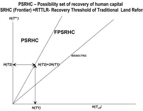
Graphically we will have figure 4:

5 _{These hypotheses might seem extremely severe but in future models (as ROCHA DE SOUSA (2005a)) they might}

PSRHC – Possibility set of recovery of human capital

FPSRHC (Frontier) =RTTLR- Recovery Threshold of Traditional Land Reform

H(TLR) H(T1) H(T**) H(T2)=2H(T1) BISSECTRIZ PSRHC H(T2) FPSRHC

FIGURE 4 – Possibility set and Recovery Threshold of Traditional Land Reform

2Q - The second question is: When will land reform be economically viable?

The same reasoning applies comparing two integrals between agronomists and workers but this time, we evaluate it forwardly using the concept of opportunity cost at the time of land reform (TLR). It is like evaluating two investments

from the same given time.

If we have, as before, the two hypotheses (TLR and HIP2) and the additional hypothesis then, it will never be viable to have LR. See ROCHA DE SOUSA (2005a in progress) which analyses also some relaxation of these hypotheses.

6. Jovanovic’s theory of firm and land reform

6.1. The idea

This section follows ROCHA DE SOUSA (2005a, ch.6; 2005e).

The story of JOVANOVIC’s (1982) model is quite simple, a firm faces cross section uncertainty (that is before entering the market) because it doesn’t know ex-ante if the firm is more or less efficient and besides in each period faces another stochastic shock.

The story goes that the ones who survive are the bigger ones, and that smaller firms have higher variance in their performance. That is as a firm grows in size and goes surviving in each period (older vintage) the probability that it goes bankrupt and exits the market diminishes.

6.2. The model’s exit decision

One part of the paper particularly important is the one which presents the exit decision.

This decision is made conditionally on the exogenous value of the opportunity cost of the fixed factor – that is if a firm exits the market receives W>0 as a compensation.

The author stresses that this W is equal across all firms, independently as successful they are in the market. The value of staying in the industry for the next period is thus given by the following Bellman equation:

(1)

V

(

x

,

n

,

t

;

p

)

=

π

(

p

_t

,

x

)

+

β

.

∫

max

[

W

,

V

(

z

,

n

+

1

,

t

+

1

;

p

]

.

P

(

dz

/

x

,

n

)

Where V(.) denotes the value of staying for an additional period, which is the profit of that period plus the maximum discounted (at rate

β

) amount of whether exiting and receiving W, or staying in the next period and receiving the

following period return. Notice that

P

(

dz

/

x

,

n

)

is the probability distribution function conditional on efficiency parameter x and the number of firms n.

6.3. A simplified deterministic model of land reform

Now we introduce our model of land reform based on JOVANOVIC (1982)

First, the production function obeys to the usual costs properties as stated in the first equation of section 4.2 as in ROCHA DE SOUSA (2005e, p.3).

Secondly, we must say that we have two factors of production: land (L) and human capital (H) both with decreasing returns.

Thirdly, we assume that the production form is the following: (2)

q

_t

=

l

(

L

_t

).

h

(

H

_t

)

,

this is multiplicatively separable in the stock of land and of human capital.

Fourth, we assume that there is only cross section uncertainty among firms (ex-ante uncertainty) and no shocks in every period, that is our

θ

is the only source of uncertainty. Of course this means that the firm in the first period comes to know whether it is efficient or not – and thus, if this is the case, it will eventually exit, when it reaches a deterministic cut-off point.

Then a new problem arises. Like the total stock of land is constant, when the agricultural firms go bankrupt, there must be done a redistribution of lands – two hypotheses arise:

LR1- Land reform of type 1- the new lands are redistributed to the new entrants (landless people).

LR2 – Land reform of type 2 – the new lands are divided equally between new entrants and current tenant holders.

6.4. The simplest model

Our problem then is to maximize expected profit subject to the production function and human capital accumulation law: (3)

_Max

[

_p

_.

_q

₋

_c

₍

_q

_).

_x

*

]

s.t. (4)

q

_t

=

l

(

L

_t

).

h

(

H

_t

)

(5) h=

∫

tq_t dt 0 .

Thus deriving (5) by the Leibnitz rule6_{, we end up with the law of motion to the stock of human capital:}

(6) h• =q_t =l(L_t).h(H_t)

We are assuming first no depreciation of human capital, and that human capital results from the accumulation of past experience (output).

We are assuming that we use mean output that is our qt is output per hectare (ha).

We have two types of agents the “small” (agent type S) or “poor” ones with low endowments (at least of start of the game) of both land and human capital, and the “big”(agent type B) or “rich” “latifundia” holders which also have a greater initial stock of human capital. Formally, we have:

(7)

_H

₍

₀

₎

S

_<

_H

₍

₀

₎

B

(8)

_L

₍

₀

₎

S

_<

_L

₍

₀

₎

B

Then our optimal control problem is resolved backwards.

6 _{PIRES (2001, pp.249) defines the Leibnitz rule, as if we have the integral}

₌

∫

) ( ) ( 2 1

).

,

(

)

(

x x

dx

y

x

f

x

A

ϕ ϕ , then the

derivative of the integral will be: ´() ´( , ). ( , ( )).´( ) ( , ₁( )).´₁( ) ) ( ) ( 2 2 2 1 x x x f x x x f dx y x f x A x x x

ϕ

ϕ

ϕ

ϕ

ϕ ϕ

∫

− + = .

In this setting the growth rate of the human capital stock is constant and pre-determined by the initial stocks (7) and (8). This is similar to what happens in some economic growth models:

(9)

h

•

=

q

_t

=

q

₀

=

l

(

L

₀

).

h

(

H

₀

)

Thus this model would not yield permanent sustained differences between “small” and “big” farmers, even though the initial starting conditions disadvantages, like there are diminishing returns to both factors:

(10)

_h

(

_H

(

0

)

S

)

_>

_h

(

_H

(

0

)

B

)

(11)

_l

(

_L

(

0

)

S

)

_>

_l

(

_L

(

0

)

B

)

and further if we have, the additional hypothesis that average productivities h(H(0)S_{) are higher for human capital’s}

small farmers than land average productivities for big farmers, then this allow us to write: (12)

_h

(

_H

(

0

)

S

)

_>

_l

(

_L

(

0

)

B

)

Thus combining (10), (11) and (12) this yields:

(13)

_l

(

_L

(

0

)

S

).

_h

(

_H

(

0

)

S

)

_>

_l

(

_L

(

0

)

B

).

_h

(

_H

(

0

)

B

)

which is equivalent to stating that, based on (9), we have:

(14) hS qS qB hB • • = > = _{0 0} .

Thus the optimal path of growth of human capital has a higher growth rate for small farmers.

6.5. The solution

We have the following optimal control problem: (15)

∫

− T o t t c q x dt q p

Max ( . ( ). *). (the functional to be maximized) s.t. (6)

h

•

=

q

_t

=

l

(

L

_t

).

h

(

H

_t

)

(the law of motion of state variable) (16)

q

(

L

₀

,

H

₀

)

=

q

₀ and (17)

λ

(

T

)

=

0

(the transversality condition) So this enables us to write the Hamiltonian:

(18)

H

(

t

,

h

,

q

,

λ

;

p

,

x

*)

=

p

.

q

_t

−

c

(

q

_t

).

x

*

+

λ

[ ]

q

_t

So the first order conditions accordingly to the Pontriagyn´s Maximum Principle (see CHIANG (1992), p. 169) are: (19)

H

=

h

=

q

_t

∂

∂

•

λ

(law of motion of state variable) (20)

=

−

•

∂

∂

_λ

h

H

(law of motion of co-state variable) (21)

λ

(

T

)

=

0

(the transversality condition) Thus if we have (19) we will have (6) as we postulated it.

So the trajectory of the state variable is known and is regulated by this simple first order differential equation. And what about the co-state (

λ

_t) ?

Starting from (20) we can calculate the equation which describes the law of motion of the co-state:

(22)

_



_



∂

∂

+

∂

∂

−

∂

∂

−

=

•

h

q

h

q

x

c

h

q

p

.

´

_q

.

*

.

λ

.

λ

(23)

.

(

´

.

*

)

.

=

0

∂

∂

−

+













∂

∂

+

•

h

q

x

c

p

h

q

q

λ

λ

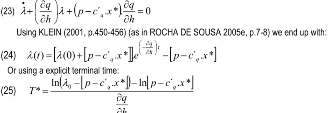
Using KLEIN (2001, p.450-456) (as in ROCHA DE SOUSA 2005e, p.7-8) we end up with:

(24)

(

t

)

[

(

0

)

[

p

c

´

.

x

*

]

]

.

e

h .t

[

p

c

´

_q

.

x

*

]

q q

−

−

−

+

=

     ∂ ∂ −

λ

λ

Or using a explicit terminal time:

(25)

(

[

]

)

[

]

h

q

x

c

p

x

c

p

T

q q

∂

∂

−

−

−

−

=

ln

´

.

*

ln

´

.

*

*

λ

0

This is the optimal terminal time for our initial problem, where the shadow value of the co-state will yield a zero value. The intuition is that the human capital resource won’t be further used because the problem ends. So, it doesn’t make sense to keep human capital for the next period, because in the next period the problem has ended.

The terminal time is a function of the starting shadow-cost (human capital salary-

λ

(

0

)

=

λ

₀) and of the margin of profit

[

p

−

c

´ x

_q

.

*

]

, which integrates the efficiency of the firm (x*) as JOVANOVIC has been using – even though in this case it is deterministic. And besides it also depends on the productivity of human capital

h

q

∂

∂

.

The law of motion of the state variable (6)=(19) is conditioned from the very start by equation (5). So, this allows us to describe the state variable human capital path as in figure 5. The control variable is qt which accumulated over

time (integral) yields the value of the state variable as it is shown on equation (5) – see again figure 5.

There is an intuition in this Model I, in stead of human capital (ht) determining production (qt) we have it the other

way round. It is the accumulation of output which leads to further human capital and this feedbacks on more output. That is we have a process of learn by doing – which results from dynamic scale economies.

8,

80

cm

dh/dt=qt

Time profile, evolution and selection of firms in MODEL I h(t) state variable ; q(t) control variable

V>W =q(pt/x0) 0 Failure Failure limit Survivor V<=W dh/dt0=q₀ T t1 dh/dT=qT dh/dt1=q1 0 . t t h=

_∫

q dt

7. Conclusion

We presented a static model which yields viable land reform if the pro-efficiency effect (of competition) dominates

over the pro-learning effect of latifundia.

The main conclusion of the dynamic models is that with the neoclassical exogenous framework there is convergence between small landholders and latifundia holders. This is a successful land reform: there is a finite time horizon that allows almost landless illiterate to catch up with rich literate farmers. In the case of endogenous growth there is never convergence thus the land reform process fails.

Another conclusion in the endogenous framework is that, by reverse causality, failed land reforms result from perpetuating initial differential human capital stocks.

In section 5, another approach is to extend ARROW (1962) learn by doing model to evaluate land reform as a structural break (or cut-off point). A condition for land reform viability is established, creating a Possibility Set for Human Capital Recovery (PSRHC).

In section 6 we simplify the theory of the firm JOVANOVIC’s (1982) model, applying it to agricultural firms to explain birth, life and death of latifundia. We establish the date and process of land reform, as a cut-off process, in which it arises from the failure of firms.

8. References

ARROW, Kenneth (1962). “The economic implications of learn by doing”, Review of Economic Studies, vol. XXIX (3), no. 80, June, pp. 155-173

BARRO, Robert and SALA-I-MARTIN, Xavier (1995), Economic growth, McGraw Hill, Singapore.

BECKER, Gary (1993), Human capital: a theoretical and empirical analysis with special reference to education, 3rd

edition, University of Chicago Press, USA (1st _{edition - 1964)}

BECKER, Gary (1996), Accounting for tastes, Harvard University Press, USA.

DE JANVRY, Alain (1981a), “ The role of Land Reform in Economic Development: Policies and Politics”, American

Journal of Agricultural Economics, May, vol. 63, pp. 384-392.

DE JANVRY, Alain (1981b), The Agrarian Questions and Reformism in Latin America, Johns Hopkins Press: Baltimore and London.

JONES, Charles I. (1995), “R&D-Based models of economic growth”, Journal of Political Economy 103 (August), 759-84.

JONES, Charles I. (1998), Introduction to economic growth, W. W Norton & Company, 1st _{edition, USA.}

JOVANOVIC, Boyan (1982), “Selection and evolution of industry”, Econometrica, vol. 50, No.3, May 1982, pp. 649-670.

KAWAGOE, Toshihiko (1999), “Agricultural land reform in post-war Japan: experience and issues”, World Bank Policy Research Working Paper 2111, May, Washington D.C.

KLEIN, Michael W. (2001), Mathematical methods for Economics, 2nd _{edition, Addison Wesley, Boston, USA.}

MANKIW, N. Gregory; ROMER, David and WEIL, David (1992), “A contribution to the empirics of economic growth”,

Quarterly Journal of Economics, 107, May, pp.407-438.

PIRES, Cesaltina (2001), Cálculo para economistas, McGraw Hill, Lisbon, Portugal.

ROCHA DE SOUSA, Miguel; SOUZA FILHO, Hildo Meirelles; BUAINAIN, António Márcio, SILVEIRA, José Maria; MAGALHÃES, Marcelo Marques (2004); “Stochastic Frontier Production Evaluation of market assisted land reform in NE Brazil”, Proceedings from the 4th _{International Symposium of DEA, 5}th _{– 6}th _{September, Aston}

University, Birmingham, UK, pp. 361-368; and Proceedings of XXXII ANPEC, 5th_-10th _{December, João}

Pessoa, Brazil.

ROCHA DE SOUSA, Miguel (2005a), Análise Económica de Reforma Agrária em contexto dinâmico, PhD Thesis in progress, Universidade de Évora, Departamento de Economia, Portugal, 144 pages, mimeo.

ROCHA DE SOUSA, Miguel (2005b), “Land reform with human capital: a note on static efficiency analysis”, mimeo,

Universidade de Évora, Departamento de Economia, Portugal, 20 pages, in progress.

ROCHA DE SOUSA, Miguel (2005c), “Land reform with human capital II: a brief extension of BHADURI’s credit model”, mimeo, Universidade de Évora, Departamento de Economia, Portugal, 11 pages, in progress.

ROCHA DE SOUSA, Miguel (2005d), “Land reform with human capital: a new analysis using the theory of economic growth”, mimeo, Universidade de Évora, Departamento de Economia, Portugal, 19 pages, in progress. ROCHA DE SOUSA, Miguel (2005e), “Land reform with human capital: a new analysis using the theory of the firm”,

mimeo, Universidade de Évora, Departamento de Economia, Portugal, 17 pages, in progress.

ROCHA DE SOUSA, Miguel (2005f), “Land reform with human capital: a new analysis using the theory of economic growth and the theory of the firm”, paper presented at the

3

rd International Conference on European and International Political and Economic Affairs, 26-28th _{May 2005 at ATINER Institute, Athens, Greece.}

ROMER, Paul (1990), “Endogenous technological change”, Journal of Political Economy, 98, October : S71-S102. SOLOW, Robert (1956), “A contribution to the theory of economic growth”, Quarterly Journal of Economics, 70, 1,

February, pp. 65-94.

SWAN, Trevor W. (1956), “Economic growth and capital accumulation”, Economic Record, 32, November, pp. 334-361.