A subjective poverty line for Portugal

(1)

A SUBJECTIVE POVERTY LINE

FOR PORTUGAL

by

Sara Gonçalves Lourenço

Dissertation submitted in partial fulfillment of the requirements for the degree of

Master of Science in Economics at the

Universidade Católica Portuguesa

Dissertation written under the supervision of Miguel Gouveia

(2)

(3)

3

A SUBJECTIVE POVERTY LINE FOR PORTUGAL

Sara Lourenço

Supervisor: Miguel Gouveia

December 28, 2017

Abstract

The aim of this thesis is to estimate a subjective poverty line for Portugal, using data collected by the PEO – Painel de Estudos Online of the Catolica Lisbon School of Business and Economics in March and November 2016. The analysis is based on a log-log regression for stated income needs (answer to a minimum income question) using as explanatory variables net monthly income, number of adults, number of children, and including a vector of other demographic characteristics of the household.

After several attempts to include other variables concerning demographic characteristics in the model, it was possible to conclude that the only significant variables to add to the model would be a set of geographic dummies depending on the area of location of the household: North, Centre, South and Islands. Finally, two regressions were run, one without any demographic characteristics and one including the location dummies. In both regressions the answer to the Minimum Income Question depends positively on Net Monthly Income, the number of adults and the number of children living in the household. Using the second model it is also possible to conclude that the answer to Minimum Income Question also depends on the location of the household, and that the answers are higher in the South than in any other region.

(4)

A SUBJECTIVE POVERTY LINE FOR PORTUGAL

Sara Lourenço

Supervisor: Miguel Gouveia

28 de Dezembro de 2017

Resumo

O objetivo desta tese é estimar uma Linha de Pobreza Subjetiva em Portugal, usando dados recolhidos pelo PEO – Painel de Estudos Online da Catolica Lisbon School of Business and Economics em Março e Novembro de 2016. Para que tal fosse possível foi usado um modelo log-log com as seguintes variáveis: rendimento mensal líquido, número de adultos e número de crianças no agregado familiar e um vetor de características demográficas do agregado familiar. Após várias tentativas de um incluir um vetor de variáveis especificas, foi possível concluir que o único conjunto de variáveis relevantes era relativamente ao local de habitação do agregado familiar, nomeadamente: Norte, Centro, Sul e Ilhas. Finalmente, foram efetuadas duas regressões, uma sem incluir nenhuma característica demográfica e outra incluindo a localização de habitação referida anteriormente. Foi possível concluir que em ambas as regressões a resposta à Questão de Rendimento Mínimo depende positivamente do rendimento mensal liquido, do número de adultos e do número de crianças que vivem no agregado familiar. Adicionalmente, usando o segundo modelo podemos concluir que estas mesmas respostas variam consoante a região de habitação do agregado familiar, nomeadamente as respostas são em média mais altas na região Sul do país do que em outra qualquer região.

Palavras-chave: Pobreza, Subjetiva, Questão de Rendimento Mínimo, Diferenciação

(5)

5

(6)

Acknowledgments

First, I would like to dedicate this thesis to my father, that wherever he is, was the main force to encourage me to finish the Master of Science with success.

I would also like to thank Professor Miguel Gouveia for all the support given along this work, only with his advice and feedback it was possible to complete this Master’s Thesis. I would also like to leave an important thank you to Professor Rita Coelho Vale for being the person collecting the data I have used in this work.

(7)

7

(8)

List of figures

Table 1: Absolute Poverty Lines, estimated by Alfredo Bruto da Costa in 1994 at 2016 prices

... 16

Table 2: Evolution of 60% of median equivalised income for Portugal between 2007-2015, updated for 2015 prices ... 16

Table 3: Relative Poverty Lines estimated by Celso Nunes (1999), updating for 2016 prices 17 Table 4: Adequate Income for Portugal, estimated by Pereirinha et al. in 2017... 17

Table 5: Subjective Equivalence Scales for Portugal, estimated by Bishop et al. in 2014 ... 18

Table 6: Distribution of the sample by gender ... 20

Table 7: Distribution of the sample by age ... 21

Table 8: Sample Statistics regarding age ... 21

Table 9: Distribution of the sample by marital status ... 21

Table 10: Distribution of the sample by level of education ... 22

Table 11: Distribution of the sample by number of persons in each household ... 22

Table 12: Distribution of the sample by number of children ... 22

Table 13: Statistics of the data regarding Net Monthly Income... 24

Graph 1: Net Monthly Income Histogram of the sample ... 25

Table 14: Statistics of the data regarding the Minimum Income Question ... 26

Figure 1: Frequency distribution of Minimum Income Question ... 26

Figure 2: Frequency distribution of Minimum Income Question truncated at 4000€ ... 27

Figure 3: Kernel density of Minimum Income Question ... 27

Table 15: Population Density of Portugal in 2014, according to Wikipedia ... 29

Figure 4: Results of regress model 1 ... 31

Table 16: Results for Subjective Poverty Lines using Model 1 ... 37

Table 17: Results of Subjective Poverty Line using Model 4 ... 38

Table 18: Equivalence Scales using Model 1 ... 38

(10)

1. Introduction and Literature Review

Since poverty is one of the main concerns in modern societies, measuring poverty is very important since it allows citizens and governments to understand the dimension of the problem and come up with policies to minimize poverty in their countries. In the European Union, the goal of reducing poverty has become clearer after the Lisbon European Council in 2000.

There are several ways to measure poverty, which will be briefly described in the next subchapters. In this thesis, the subjective poverty line approach will be studied and implemented. The subjective poverty line (SPL) is a hybrid concept. It requires that people below the SPL should consider themselves poor, and people above the SPL should consider themselves non-poor.

In this thesis, what will be tried is to apply a subjective poverty line to Portugal. I will consider as poor people those who do not have enough monetary resources to satisfy their needs. I chose to research this theme because as far as I know this approach has not been applied in Portugal. This task will be important considering the difficulties that Portugal has been through in the past few years and given that poverty is one of its current main problems, since the poverty rate in Portugal (number of people below the official poverty line) was 19% in 2016, according to Eurostat. This figure is very high compared with other European Countries.

This study will be relevant for public policies because measuring poverty is very important since it allows us to understand the dimension of the problem of poverty in each country, and therefore it becomes possible to adopt measures that will fit better the needs of each country. Also, measurement of poverty allows us to compare the levels of poverty across countries. The main objective of poverty lines is identifying people that live in poverty. The introduction of the poverty line defines the income level that separates poor and non-poor (Hagenaars and Pragg, 1985). It is also important to take into consideration that no matter what type of poverty line is used, it is always based on assumptions about the nature of poverty (Hagenaars and Pragg, 1985).

The subjective poverty line studied in this thesis should be seen as an additional source of information, since all income poverty lines are informative and should be seen as a way of complementing previous knowledge (Iceland, 2005). It should be considered that no measure is perfect, all have some problems associated with them, but so far, no uniform consensus

(11)

11

has been reached choosing the best measure (Iceland, 2005).

In this research, income will be used as the unit of measurement of poverty for mainly two reasons. The first one is the fact that income is much easier to obtain than, for instance, consumption or wealth. The second is the fact that given that my data was collected before I decided on the exact indicator I was going to use, and the variables collected are with respect to income, collecting new data would be a waste of resources since income is suitable for my analysis and income has been used by many researchers.

There are mainly three types of poverty lines: absolute, relative and subjective. Although my research focuses on Subjective Poverty Lines, I will present a brief survey of the characteristics of each. I will also explain the importance of equivalence scales in measuring poverty. At the end of this introductory chapter I will provide information on poverty lines in Portugal, in order to have some term of comparison with my results.

1.1. Absolute Poverty Line

The concept of absolute poverty is related to having insufficient resources to afford some basket of basic needs, although this implies some subjectivity in choosing what is considered as basic needs. This concept is independent of the income level in each society.

In order to measure poverty, the World Bank uses the famous dollar-a-day indicator, which was updated to $1,90 (using 2011 data) in October 2015. This poverty line had not been updated since 2008, and was changed in 2015 because it was necessary to update the concept of poverty given the changes in the cost of living across the world. This measure of the World Bank is a typical absolute poverty approach since it is a measure directly based on needs, not on society´s income.

Even in the case of absolute poverty lines, there must be updates over time, like the dollar-a-day indicator of the World Bank, it is necessary to create a better fit with real conditions. Rowntree is considered the father of the scientific study of poverty, including the definition of the absolute poverty line. In his work in 1901 book he studied poverty considering as poor the families that didn’t have enough income to insure basic biologic survivor conditions, which he called the “concept of substance” (Rowntree, 1901). While Rowntree used this absolute concept applied to England, latter, in 1965, Orshanshy used similar concepts applied to the United States, becoming also one of the reference authors on this topic (Orshanshy, 1965).

(12)

Although the use of the absolute poverty line has been losing ground throughout the years, there are some cases where they are more suitable. They are preferable in cases of comparison of societies with very dissimilar levels of income. On the other hand, it is not recommendable to use absolute poverty when the goal is to evaluate poverty in a rapid and simple way, when the idea is only to have an overview of poverty in a society (Nunes, 1999).

It is also important to note that the income elasticity associated with an absolute poverty line is always zero, since under the absolute case the poverty line is constant, which means that if the poverty lines were not updated with the evolution of the living standards of the population nowadays very few people would be considered poor (Kipatrick, 1973). It is important to take into consideration that absolute poverty lines are subject to updates due to price evolution (inflation), which are usually designed as cost of living adjustments.

1.2. Relative Poverty Line

In the case of relative poverty, the poverty line is derived by identifying people who do not have enough money to be well integrated in a society. This is usually done by taking the mean or the median income, and setting the threshold between poor and non-poor as a percentage of that value. In this way being considered poor depends on the characteristics of the society where a person lives. There is a very large number of relative poverty lines that can be calculated using the same data, since the cut-off can be defined for very different percentages. The most common relative poverty lines used are based on the median or the mean income, although there is also a discussion between which of the two statistics should be used. For example, Eurostat uses 60% of the median equivalence income in society, but other institutions may use other cut-offs.

One point in favour of using the mean as a calculation base is the simple way how it can be estimated. On the other hand, the median is robust against changes in the data and against the existence of outliers in the statistical samples of data.

The origin of the relative poverty concept is much older that we ordinarily think. Adam Smith in 1776 defined poverty as failing to have access to “not only the commodities which are indispensably necessary for the support of life, but whatever the custom of the country renders it indecent for creditable people, even of the lowest order, to be without.” (Smith, 1776). But the best-known definition of relative poverty was due to Townsend in 1979:

(13)

13

“individuals, families and groups can be said to be in poverty when they lack the resources to obtain the types of diet, participate in the activities and have the living conditions and amenities which are customary, or are at least widely encouraged or approved, in the societies to which they belong.” (Townsend, 1979).

It is usually pointed out as a reason for the evolution of relative poverty lines the fact that most authors did not agree with the concept or measures of absolute poverty. Although there are some difficulties associated with a relative poverty line, as in the definition of the cut-off point (Costa, 1994), it is much simpler and easier to calculate.

Using relative poverty lines is more indicated in cases when it is necessary to have a fast estimate. The relative approach has also been proven to have success when comparing countries with similar income levels (Nunes, 1999).

Considering the income elasticity of the relative poverty line, we face the exact opposite case of the absolute poverty, since the income elasticity is one in the relative approach. That means the relative poverty line changes in the exact same proportion as average income (assuming the relative income distribution is constant) (Kilpatrick, 1973).

1.3. Subjective Poverty Line

The subjective poverty line is derived by asking a given population what they consider to be the minimum income they should have in order not consider themselves poor. In this way, the definition of poverty is independent from the investigator and will be more compatible with society’s perspective, since it is not necessary to define the basic bundle of goods or the income threshold (Hagenaars and Praag, 1985). This definition is based on the assumption that people are the best judges of their own welfare and so the measurement of poverty should be based on their assessment. Using this approach is important because different people have different needs, and this allows us to consider this heterogeneity in the welfare judgments of individuals. Later on, a chapter will clarify what is exactly the Subjective Poverty Line.

The subjective approach was first introduced by Goedhard el at. in 1977 when they defined a method where families consider themselves poor if they do not make enough money to make ends meet, according to their opinion. This method is based on the Minimum Income Question (MIQ) (Goedhard et at, 1977). The most well-known formulation of the MIQ was created by Kapteyn in 1985: “What income level do you personally consider to be absolutely

(14)

minimal? That is to say that with less you could not make ends meet.”.

When answering the Minimum Income Question, different people may have different ideas on what it means to be poor, which will generate different interpretations of survey questions. Some responders will tend to underestimate their income, consider themselves poorer than they actually are (for example by excluding some secondary income, like family farm outputs), and other families will consider themselves richer than they actually are, overestimating their incomes (for example by ignoring some production costs). This is a major concern in developing countries (Pradhan and Ravallion, 2000).

Some problems have been pointed out to this approach like the fact that the way in which the MIQ is formulated may give rise to different results. Another problem is that the error registered in small samples is significantly high and it is also frequent to find high variances even in large samples (Citro and Michael, 1995). An additional problem with this formulation is the fact that if people believe that their answer will influence the amount of state transfers they will receive, they could strategically change their answers (Citro and Michael, 1995). It was also found that the subjective poverty line tends to vary over time (Van den Bosch et al., 1993).

As for the values of its income elasticity, when using a subjective approach, the value is between zero and one, since the poverty line increases with average income, but not in the same proportion, which means that subjective poverty line income elasticity is located somewhere between the absolute and the relative approach (Kilpatrick, 1973).

1.4. Equivalence Scales

Equivalence scales are a tool that allows one to make comparisons across different household structures by converting their members into equivalent individuals. These scales express the different structures of expenditures across households when all obtain the same level of welfare or standard of living (Lewbel and Pendakur, 2008).

There are basically three types of equivalence scales. The first are expert scales, which are obtained by letting experts identify the needs of different sized households. This is usually done by creating a basket of good which would, in theory, lead different households to the same utility value. The best-known expert equivalence scales are the OECD scale (1 to the first adult, 0,7 to the second and the next adults and 0,5 to children until 14 years old) and the Modified OECD scale (1 to the first adult, 0,5 to the second and the next adults and 0,3

(15)

15

to children until 14 years old). The problem with these scales is that they are based on judgements that usually don’t have theoretical or empirical evidence. The second type are equivalence scales derived from objective data, for example by using the share of expenditure on some goods as a proxy to the level of welfare (Deaton and Muellbauer, 1986). These scales have the problem of being extremely based on strong assumptions associated with the specific models used. The third type, and the approach that I will take in this thesis, are subjective scales that are based on survey answers, namely using the MIQ that was mentioned before.

According to a study performed in the Euro Zone countries applying subjective equivalence scales, the authors obtain scales which reflected larger economies of scale and higher relative costs of children, compared with the Modified OECD scales. They also found that the more developed a country is, the larger are the economies of scale in household size. They concluded that the cost of adding a third adult to the household was lower than the cost of adding the first child (0,18 vs 0,3) (Bishop et al., 2014).

1.5. Poverty Lines in Portugal

There are some studies that estimated poverty lines for Portugal, although based on the research conducted for this thesis there is no study that estimated a subjective poverty line. Despite this, I will briefly review what has been done in terms of absolute and relative poverty lines, and also report on a recent study about adequate income in Portugal. Finally, I will make a reference to an equivalence scale derived for Portugal using a Subjective Poverty Approach.

All the values were updated using the most recent Consumer Price Index (CPI) by using a tool available in the Instituto Nacional de Estatística (INE) website for that end1_.

In terms of absolute poverty lines, the first one estimated for Portugal was proposed by Alfredo Bruto da Costa in 1994. In his study, he differentiated between rural and urban areas and he calculated the absolute poverty lines for 1980 and 1989. The results are the following (Costa, 1994):

(16)

Table 1: Absolute Poverty Lines, estimated by Alfredo Bruto da Costa in 1994 at 2016 prices

1980 1989

Rural Areas 2779.79 €/year 3219,15 €/year

Urban Centres 3798.12 €/year 4330.05€/year

After the previous study, the next absolute poverty line for Portugal was estimated by Celso Nunes in his thesis, where he obtained the poverty lines for 1989/1990 and for 1994/1995. Updating for 2016 prices (using the same tool provided by INE), the values were respectively 6123.84 €/year and 9681.32 €/year (Nunes, 1999).

The most recent study related to absolute poverty lines was done, also in a thesis context, by António Pereira. He estimated an Orshansky Poverty Line, which is a type of absolute poverty line. The author created two poverty lines using data from 2005. One included restaurants and other not including restaurants. Updating for 2016 price the values obtained were 7512,61 €/year and 5000,69 €/year, respectively.

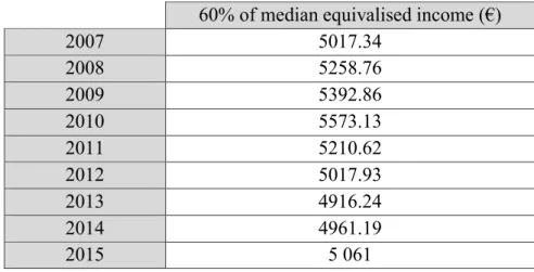
Regarding the Relative Poverty Line, in Portugal we have the common approach of Eurostat, which is taking 60% of median income. We can obtain the following information throughout the years:

Table 2: Evolution of 60% of median equivalised income for Portugal between 2007-2015, updated for 2015 prices

60% of median equivalised income (€)

2007 5017.34 2008 5258.76 2009 5392.86 2010 5573.13 2011 5210.62 2012 5017.93 2013 4916.24 2014 4961.19 2015 5 061 Source: Eurostat

(17)

17

Although there was still no updated information for 2016 in Eurostat, INE (Instituto Nacional de Estatística) has released a press stating that the value for the previous measure in 2016 was 5422€ at 2016 prices, which is equivalence to 5389.13€ in 2015 prices2_.

Adding to this data, Celso Nunes also found some results estimating Relative Poverty Lines. They can be summarized in the following table:

Table 3: Relative Poverty Lines estimated by Celso Nunes (1999), updating for 2016 prices

1989/90 1994/1995

50% Mean Income 3094.53 €/year 4343.90 €/year 50% Median Income 2565.63 €/year 3351.89 €/year

Another relevant study was performed in 2017. It estimates the Adequate Income for Portugal, which is defined as the level of income that allows having a dignified life in Portugal. The results obtained can be summarized in the following table (Pereirinha at el., 2017):

Table 4: Adequate Income for Portugal, estimated by Pereirinha et al. in 2017

2_{https://www.ine.pt/xportal/xmain?xpid=INE&xpgid=ine_destaques&DESTAQUESdest_boui=281441156&DE}

STAQUESmodo=2&xlang=en

3_{Multiply the monthly value by 14, since is the number of months of earnings in Portugal.}

Family Morphology _{Value (€)}Monthly _{Value (€)}Annual 3

Individual with 65 or more living alone 634 8876

Couple of individuals, both with 65 or more 1007 14098

Individual in active age (18-64 year) living alone 783 10962

Couple of individuals, both in active age 1299 18186

Single parent family with one underage child (12 years) 1374 19236 Couple of individuals both in active age, with one underage

child (12 years) 1796 25144

Couple of individuals both in active age, with two underage

children (2 and12 years) 2271 31794

Couple of individuals both in active age, with one adult child

(18)

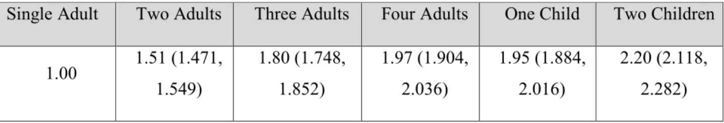
There was also an investigation conducted with data from the Euro Zone countries that allowed to find an estimate for subjective equivalence scales for a set of countries including Portugal (Bishop at el., 2014). The results are the following, depending on family size:

Table 5: Subjective Equivalence Scales for Portugal, estimated by Bishop et al. in 2014

Single Adult Two Adults Three Adults Four Adults One Child Two Children

1.00 1.51 (1.471, 1.549) 1.80 (1.748, 1.852) 1.97 (1.904, 2.036) 1.95 (1.884, 2.016) 2.20 (2.118, 2.282)

Comparing the results obtained for equivalence scales by Bishop et al. in 2014 with the Modified OECD Equivalence Scales (1 for the first adult, 0.5 for the second adult and each subsequent person older than 14 years old, 0.3 for children below 14 years old) used by Eurostat we can see that the scale for the second adult is very similar, but the weight of each additional adult decreases with the number of adults in the household. Regarding the weight of children, we can see that their weight in the work of Bishop at el. is much higher than in the Modified OECD equivalence scales. Additionally, comparing with the OECD Equivalence Scales (1 for the first adult, 0.7 for the second adult and each subsequent person older than 14 years old, 0.5 for children below 14 years old) used in Portugal to calculate the Social Integration Income, we can see that the previous study gives lower weights to adults in the household and that these weights decrease with the number of adults (not constant). In the case of children, we can see that the study gives a higher weight to them than the usual OECD scales.

(19)

19

2. Data Analysis

The source of the data used in the analysis of this thesis was collected by the PEO – Painel de Estudos Online of Catolica Lisbon School of Business and Economics with the goal of obtaining data for the 2nd_{study of the OSP – Observatório da Sociedade Portuguesa. This} process was supervised by Prof. Rita Vale Coelho. Although the dataset was not collected specifically for the purposes of my thesis, it includes all the relevant questions necessary to study and estimate a subjective poverty line in Portugal. The advantage of using this data is the fact that the survey was conducted by a credible institution. The disadvantages of this method are that sometimes one could face a problem of non-representativeness of the sample, since, as we will see later in this chapter, the number of observations for some types of demographic characteristics is disproportionately higher than for others. The data were collected in 2016, more specifically in two waves, in March and November.

The questions from the survey that I will use are the ones that contain information regarding income and sociodemographic characteristics. The complete questionnaire used by the PEO can be consulted in Portuguese in Annex I. More specifically, I will use a subset of the questions to estimate the model, but also to analyse the representativeness of the data, namely: • Minimum Income Question – What is the minimum monthly income below which you would not be able to make ends meet? (Using a sliding scale between 0 and 10,000 euros to answer this question)

• What is the net monthly income of your household? (Choose one of the following intervals: less than 500€; 500€-1000€; 1000€-1500€; 1500€-2000€; 2000€-3000€; 3000€-4000€; 4000€-5000€; more than 5000€)

• What is your gender? (female, male) • How old are you? (Indicate a number)

• What is your marital status? (single, married, nonmarital partnership, divorced, separated, widower)

• In what district do you live? (Aveiro, Beja, Braga, Bragança, Castelo Branco, Coimbra, Évora, Faro, Guarda, Leiria, Lisboa, Portalegre, Porto, Santarém, Setúbal, Viana do Castelo, Vila Real, Viseu, Região Autónoma dos Açores, Região Autónoma da Madeira)

(20)

• How many of those elements are children less than 18 years old? (none, 1, 2, 3, 4 or more)

• What is the highest education level you completed? (basic education, high school education, bachelor or undergraduate, master’s, PhD)

It was necessary to make some adjustments to the dataset since it includes a few observations of foreign citizens, which it was decided to exclude since this analysis should only include Portuguese citizens. The reason is that once the identifying question was made in terms of nationality there is no way to know if the foreign respondents were or not residents in Portugal. A few observations were also eliminated from the dataset that indicated that there was no adult living in the household, which was considered to be a mistake in answering the survey. There were also 9 observations that were dropped since the answer to the Minimum Income Question was zero, which makes no sense since no one can live with zero income. After these few modifications the dataset ended up with 1599 observations.

To initiate the analysis, the first step was looking at the distribution of sociodemographic variables to understand how representative the data is.

As it is possible to see in the following table that there is a significant difference between the number of females and males in the sample, as almost 70% of the observations are females. According to INE (Instituto Nacional de Estatística) the Portuguese population over 17 years old was composed in 2016 by 53.38% females and 46.62% males, which contrasts with the composition of the sample used.

Table 6: Distribution of the sample by gender

Frequency Percentage Female 1091 68.23%

Male 508 31.77%

Total 1599 100.00%

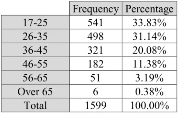
Regarding the age of participants, we can see in the next table that the observations concentrate in the younger three classes. The frequency of the observation is reduced in the older classes, and the number of individuals in the last two classes is not even 4%. The mean sample value for age is around 33 years old, which gives us again the indication that the sample is mainly composed by younger generations, since the mean age value in Portugal was 43,9 in 2016 according to demographics statistics of INE (Instituto Nacional de Estatística).

(21)

21

Additionally, according to INE in 2016, 13,99% of population between 0-14, 64,90% between 15 and 64 and 21,11% over 65 years old, which also contrasts with the sample used since there is a lack for older people in the sample, as well for the population below 17. Since this is a questionnaire it is normal that no minors are allowed to respond.

Table 7: Distribution of the sample by age

Table 8: Sample Statistics regarding age

When we look at the marital status of the participants we can observe that a large majority of the sample is single, which is normal given that there is a high concentration of younger people in the sample. According to the information collected in Censos 2011 and using as source PORDATA, in 2011 there were in Portugal 40.46% single individuals, 46.63% married, 7.3% widowed and 5.62% divorced, which (assuming a similar structure in 2016) proves that there is a significant difference between the sample and the population, although the percentage of divorced people is similar to the one in the sample.

Table 9: Distribution of the sample by marital status

Frequency Percentage Single 964 60.29% Married 300 18.76% Nonmarital Partnership 215 13.45% Separated 14 0.88% Divorced 94 5.88% Widower 12 0.75% Total 1599 100.00% Frequency Percentage 17-25 541 33.83% 26-35 498 31.14% 36-45 321 20.08% 46-55 182 11.38% 56-65 51 3.19% Over 65 6 0.38% Total 1599 100.00% Mean 32.62 Standard Deviation 10.89 Maximum 72 Minimum 17 Median 30

(22)

Regarding the level of education of the participants we can see that the majority has a high level of education, with the majority of respondents having a university degree (bachelor, undergraduate, master or PhD). According to the information available in PORDATA, in 2016, 7.85% of the population had not completed basic education, 53.97% had basic education (first, second and third cycles), 20.38% had high school education and 17.80% had higher education, which implies that the sample used in this analysis is much more educated than the population, since it has a higher percentage of respondents with higher education and very few with basic education.

Table 10: Distribution of the sample by level of education

Frequency Percentage

Basic education 48 3.00%

High school education 567 35.46% Barchelor or Undergraduate degree 689 43.09%

Master degree 279 17.45%

PhD degree 16 1.00%

Total 1599 100.00%

Looking at the composition of each household, in the following table we can see the distribution of the number of persons in each household:

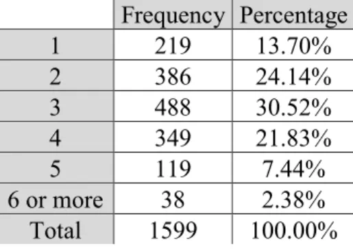
Table 11: Distribution of the sample by number of persons in each household

Frequency Percentage 1 219 13.70% 2 386 24.14% 3 488 30.52% 4 349 21.83% 5 119 7.44% 6 or more 38 2.38% Total 1599 100.00%

We can also see the number of children, under 18 years old, in each household:

Table 12: Distribution of the sample by number of children

Frequency Percentage 0 1033 64.60% 1 392 24.52% 2 133 8.32% 3 32 2.00% 4 or more 9 0.56% Total 1599 100.00%

(23)

23

By analysing the two previous tables we can see that most participants live in a household with less than 4 persons, and in a large majority of these households there are no children. This fact was expected given that most participants are single and of a young age. In the sample, the average number of persons per household is approximately 2.92, on other hand, according to PORDATA the average number of persons per household in 2016 in Portugal was 2.5. Also, according to the same source in 2016 in Portugal, 64.17% of households have no children, 21.18% have one child, 12.47% have 2 children and 2.18% have 3 or more children, which in this case means that the sample doesn’t suffer from having large differences from the population.

It is important to notice that to conduct this data analysis, given the structure of population in Portugal (small number of family members and children per couple), it was assumed that the maximum number of adults in each household was 6 and the maximum number of children was 4. This is an assumption since in the questionnaire respondents had to answer the number of children per household. The answers were provided in classes and the last class was 4 or more. Similarly, for the number of members in each household, the last class was 6 or more. This means that there may be households with a larger number of members, but that situation should be rare, since only 2.36% of the respondents said that lived in a household with 6 or more members.

Given the conclusions obtained from the demographic analysis of the sample, we can see that the observations are not equally sampled across the different sociodemographic characteristics of the population. It may not possible to fully understand the extent of this fact, but it should be taken into consideration when analysing the results of the analysis.

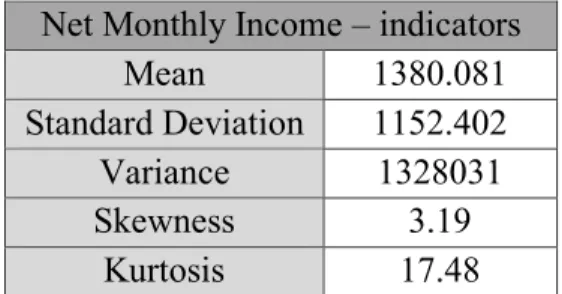
When we analyse the statistics for the net monthly income reported by the participants we can reach some conclusions by looking at the next table and ensuing graphs. The mean monthly income of the sample used in this analysis is 1378.58 € per household (sum of all sources of income in the household). To analyse the sample dispersion, we can see that the standard deviation is 1150.47 €. Regarding the skewness measure we can see that it is positive and larger than 1 which indicates that the right tail of the distribution is longer than the left. When looking to the kurtosis measure we can see that is positive which means that our sample follows a leptokurtic distribution, which is less concentrated and with fatter tails than the normal distribution.

(24)

Regarding the distribution of net monthly income by the classes we can observe in the following histogram that the majority of observation are in the classes 500-1000 and 1000-1500. I used the assumption that the top of the income distribution followed a Pareto distribution in order to estimate the mean of the upper (open) class. Using the distribution upwards of 3000€, I obtained a mean point estimate for the upper class of 8000€.

Table 13: Statistics of the data regarding Net Monthly Income

Net Monthly Income – indicators

Mean 1380.081

Standard Deviation 1152.402

Variance 1328031

Skewness 3.19

(25)

25

Graph 1: Net Monthly Income Histogram of the sample

When we analyse the statistics for the answers given to the minimum income question we can reach some conclusions by looking at the next table and associated graphs. The mean income

9,95% 36,44% 23,13% 13,74% 5,595% 1,525% 50 0 1000 1500 200 0 300 0 400 0 5000 800 0 0,5% _0,1242% 10% 20% 30% 40%

(26)

of the sample used in this analysis is 1035.32€ per household (sum of all sources of income in the household), which means that on average the participants think that their minimum income could be lower than the one they have in reality. To analyse the sample dispersion, we can see that the standard deviation is 828.68€, a value that indicates that the dispersion in this question is lower than the distribution of net monthly income. Regarding the skewness and the kurtosis measure we can reach the same conclusion as in the net monthly income analysis, but in this case both measures are even more positive.

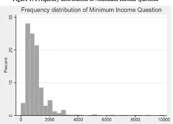
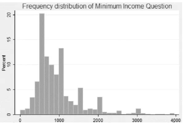
The distribution of the answers to the minimum income question we can observe that most of the observations are between 0 and 2000 euros per household. In order to observe where the majority of observation are concentrated I decided to present also a truncated graph to 4000. To run the kernel density estimation for the minimum income question, I set the halfwidth kernel to 3000 in order to get a smoother distribution than using the default width.

Table 14: Statistics of the data regarding the Minimum Income Question

Minimum Income Question – indicators

Mean 1035.32

Standard Deviation 828.68

Variance 686708.7

Skewness 4.28

Kurtosis 32.23

(27)

27

Figure 2: Frequency distribution of Minimum Income Question truncated at 4000€

(28)

3. Methodology

The aim of this thesis is to estimate a subjective poverty line for Portugal. To do that it is necessary to define a regression model that explains the relationship between the minimum income response and the household monthly income, taking also into consideration some household characteristics that could affect the answers given. The analysis proceeded by using a slightly adapted version of the log-linear relationship used by Robert J. Flik and Bernard M. S. Van Pragg (1991). The model was specified as:

𝑙𝑜𝑔(𝑀𝐼𝑄_𝑖) = 𝛼₁+ 𝛼₂log(ⅈ𝑛𝑐_𝑖) + 𝛼₃log(𝑎𝑑𝑢𝑙𝑡𝑠_𝑖) + 𝛼₄log(𝑘ⅈ𝑑𝑠_𝑖) + ∑ 𝛼_𝑗𝑋_𝑗𝑖 𝑗

where:

MIQ – are the answers to “What is the minimum monthly income below which you would not be able to make ends meet?”

inc – is the household monthly income reported by respondents adults – is the number of adults in the household

kids – is the number of kids below 18 years old in the household plus 1 (since there are some households with no children, it was necessary to add one unit to make possible to apply the logarithm)

X – is a vector that can include some demographic characteristic of the household

This model specification differs from the original one by Flik and Van Pragg since in this case the number of adults and children was included separately. In their original work they only used family size as a variable. Another difference is that it includes the X vector that could include several household characteristics, and which will be explored further later.

In order to get subjective poverty lines for Portugal depending on the household composition (and demographic characteristics) it is necessary to set 𝑙𝑜𝑔(𝑀𝐼𝑄𝑖) equal to 𝑙𝑜𝑔(ⅈ𝑛𝑐𝑖), obtaining:

log(𝑀𝐼𝑄_𝑖∗) =𝛼1+ 𝛼3log(𝑎𝑑𝑢𝑙𝑡𝑠𝑖) + 𝛼4log(𝑘ⅈ𝑑𝑠𝑖) + ∑ 𝛼𝑗 𝑗𝑋𝑗𝑖 1 − 𝛼₂

Using the previous equation this work focus on trying to understand the impact of monthly income, family size (number of adults and children) and other demographic factors in the answers given to the minimum income question. More specifically, it is analysed if there is

(29)

29

some kind of systematic regional variation in the data. A second option is to analyse if there is a systematic pattern in the data regarding population density.

Several experiences were performed in order to include a demographic characteristic of the households in the model. More specifically the geographic location of each household was included in the model, in order to try to understand if that could be relevant explaining the answers. To do this it was necessary to create several dummies. In a first analysis, this process was followed for each district.

A second analysis relied on aggregate geographic locations, by region: North (Viana do Castelo, Braga, Vila Real, Bragança and Porto), Centre (Aveiro, Viseu, Guarda, Coimbra and Castelo Branco), Lisbon Area (Lisboa, Leiria, Setúbal and Santarém), Alentejo (Beja, Évora and Portalegre), Algarve (Faro), Madeira and Açores.

A third, analysis tried an even broader aggregation of regions by North (Viana do Castelo, Braga, Vila Real, Bragança, Porto, Aveiro, Viseu and Guarda), Centre (Lisboa, Leiria, Coimbra, Castelo Branco, Santarém and Portalegre), South (Faro, Beja, Évora and Setúbal) and Islands (Madeira and Açores). The last case was the only option that generated relatively acceptable results, and then only if one assumed a significance level of 10%.

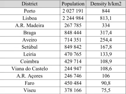
Since none of geographic location variables used had a considerable statistical significance, the next attempt was to include a population density variable. Since it was extremely difficult to find data on PORDATA or INE, information available on Wikipedia for 2014 was used. It was possible to obtain the following table:

Table 15: Population Density of Portugal in 2014, according to Wikipedia

District Population Density h/km2

Porto 2 027 191 844 Lisboa 2 244 984 813,1 A.R. Madeira 267 785 334 Braga 848 444 317,4 Aveiro 714 351 254,4 Setúbal 849 842 167,8 Leiria 470 765 133,9 Coimbra 429 714 108,9 Viana do Castelo 244 947 108,6 A.R. Açores 246 746 106 Faro 450 484 90,8 Viseu 378 166 75,5

(30)

Santarém 454 456 67,4 Vila Real 207 184 47,9 Castelo Branco 195 949 29,4 Guarda 160 931 29,2 Évora 167 434 22,6 Bragança 136 459 20,7 Portalegre 118 952 19,6 Beja 152 706 14,9

Then the next step was introducing several dummies in the regression depending on the population density of each location, namely:

• More than 500

• Between 250 and 500 • Between 100 and 250 • Between 50 and 100 • Less than 50

In this case the results also indicated we should keep the restricted model instead of the one with the population density variables.

In the next chapter it is possible to see the results obtained in each of the attempts described above. Finally, the results of the tests indicate we should keep the restricted model, and the one with large aggregate regions.

Consequently, the two following models are estimated by OLS:

• 𝑙𝑜𝑔(𝑀𝐼𝑄_𝑖) = 𝛼1+ 𝛼2log(ⅈ𝑛𝑐𝑖) + 𝛼3log(𝑎𝑑𝑢𝑙𝑡𝑠𝑖) + 𝛼4log(𝑘ⅈ𝑑𝑠𝑖)

• 𝑙𝑜𝑔(𝑀𝐼𝑄𝑖) = 𝛼1+ 𝛼2log(ⅈ𝑛𝑐𝑖) + 𝛼3log(𝑎𝑑𝑢𝑙𝑡𝑠𝑖) + 𝛼4log(𝑘ⅈ𝑑𝑠𝑖) + 𝛼5𝑁𝑜𝑟𝑡ℎ𝑖+ 𝛼6𝐶𝑒𝑛𝑡𝑟𝑒𝑖+ 𝛼7𝑆𝑜𝑢𝑡ℎ𝑖

Note that in the second model it is necessary to exclude one of the dummy variables in order to avoid the dummy trap. In this case the omitted category is “the Islands”.

Before estimating the two models, one can expect both 𝛼2, 𝛼3 and 𝛼4 to be positive, since the more monthly income a household has the higher would be the income that they understand to be necessary to satisfy their needs. Also, the more adults and children live in the household the higher the amount of income necessary to face monthly expenses.

(31)

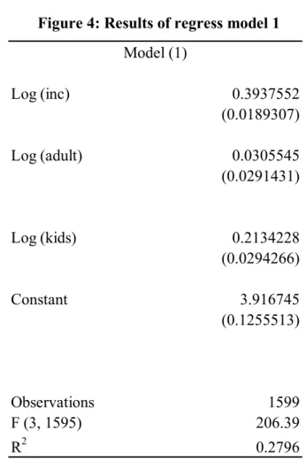
31 0.3937552 (0.0189307) 0.0305545 (0.0291431) 0.2134228 (0.0294266) 3.916745 (0.1255513) 1599 206.39 0.2796 F (3, 1595) R2 Model (1) Log (inc) Log (adult) Log (kids) Constant Observations

4. Results

4.1. Regressions' Results

The goal of this chapter is to provide the results for the estimation of each equation and to understand which of the following models should be used for the analyses in this thesis. To begin let’s analyse the equation and their respective results without insert any variable in vector X:

1) 𝑙𝑜𝑔(𝑀𝐼𝑄_𝑖) = 𝛼₁+ 𝛼₂log(ⅈ𝑛𝑐_𝑖) + 𝛼₃log(𝑎𝑑𝑢𝑙𝑡𝑠_𝑖) + 𝛼₄log(𝑘ⅈ𝑑𝑠_𝑖) It was possible to obtain the following results:

Figure 4: Results of regress model 1

Given the previous results, it is possible to conclude that monthly income and number of children are statistically significant variables. On other hand the number of adults is not statistically significant.

Making a brief interpretation of the parameter values estimated, it is possible to conclude that on average an increase of 1% in the monthly income of a household would increase the answer to Minimum Income Question by 0,39%.

(32)

Looking at the impact of changing the number of adults per household, we can observe this impact using two approaches. The first one consists in increasing by one the number of adults in each household. Using these methods, it was possible to conclude that the predicted answer to Minimum Income Question would increase on average 10.51€/month or 147.08€/year. The second approach consists in assessing the impact of changing by one the number of adults at the the average observation, i.e. where all explanatory variables are at their averages. In this case it was possible to observe that increasing the number of adults by one would generate an increase of 9.85€/month or 137.87€/year.

Treating the impact of changing the number of children in the exact same way we have done for adults, it was possible to conclude that, using the first method, the answer to Minimum Income Question would increase on average 113.68€/month or 1591.66€/year. Using the second method it was possible to conclude that we would observe an increase of 107.81€/month or 1509.31 €/year.

Let’s now work on the option of including dummies for each district in the model, is important to notice that a decided to left out the dummy for Autonomous Region of Madeira, to avoid the dummy trap. So, we would obtain the following regression:

2) 𝑙𝑜𝑔(𝑀𝐼𝑄𝑖) = 𝛼1+ 𝛼2log(ⅈ𝑛𝑐𝑖) + 𝛼3log(𝑎𝑑𝑢𝑙𝑡𝑠𝑖) + 𝛼4log(𝑘ⅈ𝑑𝑠𝑖) + 𝛼5𝑎𝑣𝑒ⅈ𝑟𝑜𝑖+ 𝛼₆𝑏𝑒𝑗𝑎_𝑖+ 𝛼₇𝑏𝑟𝑎𝑔𝑎_𝑖+ 𝛼₈𝑏𝑟𝑎𝑔𝑎𝑛ç𝑎_𝑖+ 𝛼₉𝑐𝑎𝑠𝑡𝑒𝑙𝑜𝑏𝑟𝑎𝑛𝑐𝑜_𝑖+ 𝛼₁₀𝑐𝑜ⅈ𝑚𝑏𝑟𝑎_𝑖+ 𝛼₁₁𝑒𝑣𝑜𝑟𝑎_𝑖+ 𝛼₁₂𝑓𝑎𝑟𝑜_𝑖+ 𝛼₁₃𝑙𝑒ⅈ𝑟ⅈ𝑎_𝑖+ 𝛼₁₄𝑙ⅈ𝑠𝑏𝑜𝑎_𝑖+ 𝛼₁₅𝑝𝑜𝑟𝑡𝑎𝑙𝑒𝑔𝑟𝑒_𝑖+ 𝛼₁₆𝑝𝑜𝑟𝑡𝑜_𝑖+ 𝛼17𝑠𝑎𝑛𝑡𝑎𝑟é𝑚𝑖+ 𝛼18𝑠𝑒𝑡𝑢𝑏𝑎𝑙𝑖+ 𝛼19𝑣ⅈ𝑎𝑛𝑎𝑐𝑎𝑠𝑡𝑒𝑙𝑜𝑖+ 𝛼20𝑣ⅈ𝑙𝑎𝑟𝑒𝑎𝑙𝑖+ 𝛼21𝑣ⅈ𝑠𝑒𝑢𝑖+ 𝛼₂₂𝑎ç𝑜𝑟𝑒𝑠_𝑖

(33)

33 0.3859745 Lisboa 0.0640449 (0.019382) (0.0739862) 0.0394077 Portalegre -0.2215404 (0.0295397) (0.1394851) Porto 0.021711 0.2194617 (0.0791354) (0.0295811) Santarém 0.0045721 0.0257997 (0.0977921) (0.0886107) Setúbal 0.0705334 0.1683544 (0.0826354) (0.1271986) Viana do Castelo 0.0388709 0.0153682 (0.1188383) (0.091553) Vila Real -0.1484108 -0.0670398 (0.1295048) (0.1174955) Viseu -0.0534994 0.1168412 (0.1161811) (0.0884546) Açores -0.0095497 0.1403847 (0.1063632 (0.1029484) Constant 3.917776 0.1575852 (0.1454224) (0.1043298) -0584703 (0.1294239) Observations 1599 F (22, 1576) 29.22 -0058747 0.2897 (0.1035628) Model (2) Log (inc) Log (adult) Log (kids) R2 Aveiro Beja Braga Castelo Branco Coimbra Évora Faro Guarda Leiria

It is necessary to do a global significance test of the dummies, since they only make sense together. A likelihood-ratio test was used to choose between this model or model 1. The test resulted in a p-value of 0.2580 which is large, meaning that this model should be dropped, since the model without the vector X is better.

Another approach taken was by introducing dummy variables in the model to aggregate geographic location by regions: North (Viana do Castelo, Braga, Vila Real, Bragança and Porto), Centre (Aveiro, Viseu, Guarda, Coimbra and Castelo Branco), Lisbon Area (Lisboa, Leiria, Setúbal and Santarém), Alentejo (Beja, Évora and Portalegre), Algarve (Faro), Autonomous Region of Madeira and Autonomous Region Açores. Again, in this case the Autonomous Region of Madeira is the omitted category. So, we obtain the following

(34)

0.3904044 (0.0192974) Alentejo 0.0732223 (0.0894117) 0.0363129 (0.0293822) Algarve 0.1575284 (0.1044706) 0.2129808 Açores -0.0100728 (0.029456) 0.1065076 North 0.0157381 3.891757 (0.0758902) (0.145073) Centre 0.031282 (0.0775181) 1599 Lisbon Area 0.056347 69.32 (0.0731524) 0.2819 Constant Observations F (9, 1589) R2 Log (inc) Log (adult) Log (kids) Model (3) regression:

3) 𝑙𝑜𝑔(𝑀𝐼𝑄𝑖) = 𝛼1+ 𝛼2log(ⅈ𝑛𝑐𝑖) + 𝛼3log(𝑎𝑑𝑢𝑙𝑡𝑠𝑖) + 𝛼4log(𝑘ⅈ𝑑𝑠𝑖) + 𝛼5𝑛𝑜𝑟𝑡ℎ𝑖+ 𝛼6𝑐𝑒𝑛𝑡𝑟𝑒𝑖+ 𝛼7𝑙ⅈ𝑠𝑏𝑜𝑛𝑎𝑟𝑒𝑎𝑖+ 𝛼8𝑎𝑙𝑒𝑛𝑡𝑒𝑗𝑜𝑖+ 𝛼9𝑎𝑙𝑔𝑎𝑟𝑣𝑒𝑖+ 𝛼10𝑎ç𝑜𝑟𝑒𝑠𝑖

The following results were obtained:

In order to decide if this regression should be kept, a likelihood-ratio test of this model against model 1 was performed. These results for the p-value in this test were 0,5359, meaning that this model should be dropped, since the model without the vector X is better.

The last attempt to introduce geographic location in the model was made by using a broader definition of regions: North (Viana do Castelo, Braga, Vila Real, Bragança, Porto, Aveiro, Viseu and Guarda), Centre (Lisboa, Leiria, Coimbra, Castelo Branco, Santarém and Portalegre), South (Faro, Beja, Évora and Setúbal) and Islands (Madeira and Açores). Letting the dummy regarding the Islands out, results, in the following model:

4) 𝑙𝑜𝑔(𝑀𝐼𝑄𝑖) = 𝛼1+ 𝛼2log(ⅈ𝑛𝑐𝑖) + 𝛼3log(𝑎𝑑𝑢𝑙𝑡𝑠𝑖) + 𝛼4log(𝑘ⅈ𝑑𝑠𝑖) + 𝛼5𝑛𝑜𝑟𝑡ℎ𝑖+ 𝛼₆𝑐𝑒𝑛𝑡𝑟𝑒_𝑖+ 𝛼₇𝑠𝑜𝑢𝑡ℎ_𝑖

(35)

35 0.3894736 (0.0191243) 0.0370584 (0.0293232) 0.2132117 (0.0294019) North 0.0145268 (0.0575376) Centre 0.055055 (0.0557813) South 0.1108518 (0.061655) 3.893081 (0.1362442) 1599 104.62 0.2828 F (6, 1592) R2 Model (4) Log (inc) Log (adult) Log (kids) Constant Observations

In order to decide if this regression should be used, a likelihood-ratio test was again made to choose between this model or model 1, obtaining a p-value in this test of 0.0712 which means that using a significance level of 10%, we should keep this model.

Looking at the results, we can see that the variables number of adults and the dummies for north and centre are not statistically significant, given a significance level of 10%.

In a brief interpretation of the values obtained for the parameter estimates, it is possible to conclude that on average an increase of 1% in monthly income of a household would increase the answer to the Minimum Income Question by 0,4%.

Looking at the impact of changing the number of adults per household, we can observe this impact using the two approaches previously explained in the first model. The first one would lead us to conclude that increasing by one the number of adults in each household would increase the predicted answer to the Minimum Income Question on average by 12.77€/month or 178.75€/year. Using the second approach would generate an increase of 11.96€/month or

(36)

0.3911428 (0.0191306) 0.033633 (0.0293109) 0.2143773 (0.0294819) More than 500 0.0405025 (0.0420458) Between 250 and 500 0.0048547 (0.0510655) Between 100 and 250 0.049149 (0.046569) Between 50 and 100 0.0310973 (0.0582874) 3.899738 (0.1295127) 1599 88.62 0.2805 F (7, 1591) R2 Model (5) Log (inc) Log (adult) Log (kids) Constant Observations

167.43€/year in the answer to the Minimum Income Question.

Analysing the impact of changing the number of children in the exact same way, it was possible to conclude that using the first method the would increase the answer to the Minimum Income Question on average by 113.63€/month or 1590.77€/year. Using the second method it was possible to conclude that we would observe an increase of 97.90€/month or 1370.65€/year.

Regarding the dummies we can see that living in the North increases the answer to the MIQ by 1.45%, living in Centre by 5.5% and in the South by 11,09%.

To complement these attempts to introduce dummies in the model, it was decided to try to include a set of dummy variables differentiating for population density, using the assumptions mentioned in the previous chapter. The following model was estimated:

5) 𝑙𝑜𝑔(𝑀𝐼𝑄_𝑖) = 𝛼₁+ 𝛼₂log(ⅈ𝑛𝑐_𝑖) + 𝛼₃log(𝑎𝑑𝑢𝑙𝑡𝑠_𝑖) + 𝛼₄log(𝑘ⅈ𝑑𝑠_𝑖) +

𝛼5𝑚𝑜𝑟𝑒5000𝑖+ 𝛼6𝑏𝑒𝑡250𝑎𝑛𝑑500𝑖+ 𝛼7𝑏𝑒𝑡100𝑎𝑛𝑑250𝑖 + 𝛼8𝑏𝑒𝑡50𝑎𝑛𝑑100𝑖 With the following results:

(37)

37

Once again, in order to decide if this regression should be considered, a likelihood-ratio test was again made to choose between this model or model 1, obtaining a p-value in this test of 0.7452 meaning that this model should be dropped, since the model without the vector of dummies is better.

The next step is then estimate the subjective poverty lines for the two following models: 1) 𝑙𝑜𝑔(𝑀𝐼𝑄_𝑖) = 𝛼₁+ 𝛼₂log(ⅈ𝑛𝑐_𝑖) + 𝛼₃log(𝑎𝑑𝑢𝑙𝑡𝑠_𝑖) + 𝛼₄log(𝑘ⅈ𝑑𝑠_𝑖)

4) 𝑙𝑜𝑔(𝑀𝐼𝑄𝑖) = 𝛼1+ 𝛼2log(ⅈ𝑛𝑐𝑖) + 𝛼3log(𝑎𝑑𝑢𝑙𝑡𝑠𝑖) + 𝛼4log(𝑘ⅈ𝑑𝑠𝑖) + 𝛼5𝑁𝑜𝑟𝑡ℎ𝑖+ 𝛼₆𝐶𝑒𝑛𝑡𝑟𝑒_𝑖+ 𝛼₇𝑆𝑜𝑢𝑡ℎ_𝑖

The following equation comes from the first model: 𝑙𝑜𝑔(𝑀𝐼𝑄𝑖) =

3,9167 + 0,0306 log(𝑎𝑑𝑢𝑙𝑡𝑠_𝑖) + 0,2134 log(𝑘ⅈ𝑑𝑠_𝑖) 1 − 0,3936

Using several family morphologies to calculate the poverty lines and multiplying for 14 in order to obtain annual values, it was possible to obtain the follow:

Table 16: Results for Subjective Poverty Lines using Model 1

Family Morphology Subjective Poverty Line (€)

Single Adult Individual 8937.36

Couple of Adult Individuals 9074.16

Couple of Adults plus one children 10088.20 Couple of Adults plus two children 10733.13 Couple of Adults plus three children 11215.57 Single Individual plus one children 9936.12 Single Individual plus two children 10571.33 Single Individual plus three children 11046.49

These are the main results obtained in this thesis. The model without dummies show us that adding another child to the household, requires a larger increase of subjective income than increasing the household size by one adult.

In the case of the second model, we obtain the following equation: 𝑙𝑜𝑔(𝑀𝐼𝑄𝑖) =

3,8931+0,0371 log(𝑎𝑑𝑢𝑙𝑡𝑠_𝑖)+ 0,2132 log(𝑘𝑖𝑑𝑠𝑖)+ 0,0145 𝑛𝑜𝑟𝑡ℎ𝑖+ 0,055 𝑐𝑒𝑛𝑡𝑟𝑒𝑖+0,1109 𝑠𝑜𝑢𝑡ℎ𝑖

1−0,3895

(38)

Table 17: Results of Subjective Poverty Line using Model 4

Family Morphology Subjective Poverty Line (€)

Single Adult Individual 8233.46

Couple of Adult Individuals 8385.46

Couple of Adults plus one children 9315

Couple of Adults plus two children 9905.81

Couple of Adults plus three children 10347.6

Single Individual plus one children 9146.15

Single Individual plus two children 9726.24

Single Individual plus three children 10160

Living in the North comes multiplied by 1.024035326 Living in the Centre comes multiplied by 1.094272862 Living in the South comes multiplied by 1.199199657

Given the values obtained, it was decided that the second model should also be taken into consideration since there are considerable differences between the subjective income obtained for families living in the North, Centre, South or Islands. It is possible to see that, given the data used in this thesis, respondents consider that it is more expensive to live in South than in the rest of the country.

It should also be taken into consideration the fact that the test for this model resulted in a value of p-value larger than 5%, but lower than 10%, which implies that the results of this model could be considered as not very robust.

4.2. Equivalence Scales from these models

In this subchapter the equivalence scales that were possible to obtained from models 1 and 4 are presented.

For model 1, without location differentiation, it was possible to obtain the following equivalence scales:

Table 18: Equivalence Scales using Model 1

Adults Children E.S.

1 0 1 2 0 1.0153 2 1 1.1288 2 2 1,2009 1 1 1.1118 1 2 1.1828

(39)

39

For model 4, with location differentiation, it is important to considerer that equivalence scales would not differ from the region of living, the following scales were obtained:

Table 19: Equivalence Scales using Model 4

It is possible to observe that the equivalence scales of the two models are not very different. Given the demographic composition of the sample it is possible to believe that the subjective poverty line is not very biased, but the details, more specifically the equivalence scales have a low degree of reasonableness. These conclusions are reached since these equivalence scales are very distant from the official equivalence scales, more specifically they are extremely low comparing with the OECD Equivalence Scale (1,0.7,0.5) and the Modified OECD Equivalence Scale (1,0.5,0.3).

4.3. Comparation with other Poverty Lines

This subchapter presents a brief comparison of the results obtained with the existent poverty lines in Portugal. For comparation proposes the subjective poverty line without location differentiation is used.

Comparing with the main results obtained for Absolute Poverty Line by Costa in 1994 for Portugal, it is possible to conclude that the subjective poverty line in this thesis is much larger than these lines, making the calculations with the absolute poverty line obtained for 1989 for Urban Centres in Portugal, we came to the conclusion than this subjective poverty line is 51,55% (8937,36−4330,05

8937,36 ) higher, which given the fact that the absolute poverty line of Alfredo Bruto da Costa is in 2016 prices is a large difference.

Looking in the perspective of relative poverty lines, we can see that looking to the official Eurostat measure of 60% of median income for 2016 that was 5442 euros €/year, the values obtain in this subjective poverty line are considerable larger, more specifically 39,11%

Adults Children E.S.

1 0 1 2 0 1.0185 2 1 1.1314 2 2 1.2031 1 1 1.1109 1 2 1.1813

(40)

(8937,36−5442

8937,36 ) higher, since this is the official measure for poverty in Portugal, we can consider that these results could be very significant.

The most important comparison to make concerns the results obtained by Pereirinha et al. in 2017 regarding the Adequate Income for Portugal, which is in some way a subjective approach to poverty in Portugal. In their study they differentiated households by age. In this case the case closest to the single individual adult is an individual in active age living alone, which result in 783€/month and 10962€/year. The results in this present thesis are lower than the results obtained by Pereirinha et al., we can see that the results obtained in this thesis are 22,65% (8937,36−10962

(41)

41

5. Conclusion

This thesis studied the poverty lines using the subjective approach. To do that it used data collected in 2016 by PEO – Painel de Estudos Online of Catolica Lisbon School of Business and Economics, with a total of 1599 individual observations.

Given some characteristics of the sample used to conduct this analysis it is important to keep in mind that, we could be faced with a biased sample, since some of the sample characteristics do not match the characteristics of the Portuguese population. In particular, the sample collected is mainly composed by young and single individuals. Despite this fact, the results obtained can be seen as an additional source of information to analyse poverty in Portugal, since the poverty lines estimated are still informative.

It was possible to see that using a model without geographic differentiation, a single adult individual would need 8937.36€/year. We can also conclude that, as expected, the answer to the minimum income question depends positively on monthly income, number of adults and number of children in a household.

Additionally, using a model with geographic differentiation for location, it was possible to conclude that a single adult individual living in North would need 8431,35€/year, the same single adult individual living in Centre would need 9009,65€/year, a single adult individual living in South would need 9873,56€/year and finally a single adult individual living in the Islands would need 8233,46€/year. These results show that depending on the location of the household the amount that each considers to be the income minimum not to be poor differs. The results above concern a specific household structure, a single adult individual, but the models estimated can provide us with results for any household composition.

It is possible to conclude that given the demographic structure of the sample it was not possible to obtained unbiased results for equivalence scales, although I believe that the results from Subjective Poverty Lines aren’t very biased.

To conclude, I believe that these results, along with the recent results obtained by Pereirinha et al. for an Adequate Income for Portugal, reinforce the idea that maybe the official measures to evaluate poverty in Portugal (more precisely the Eurostat 60% median of income) are not suitable to measure the real needs of the population since they lack what is necessary for individuals to consider themselves not poor.

(42)

6. References

[1] BISHOP, John A., Andrew Grodner, Haiyong Liu and Ismael Ahamdanech-Zarco. "Subjective Poverty Equivalence Scales for Euro Zone Countries". The Journal of Economic Inequality, Volume 12, Issue 2 (June 2014): 265–278

[2] CITRO, Constance and Robert Michael - Measuring Poverty: a New Approach. National Research Council, 1995

[3] COSTA, Alfredo Bruto da. "The Measurement of Poverty in Portugal". Department of Social Sciences, Portuguese Catholic University, Volume 4, Issue 2 (May 1994): 95-115

[4] DEANTON, Angus and John Muellbauer. "On Measuring Child Costs: With Applications to Poor Countries". Journal of Political Economics, Volume 94, Number 4 (August 1986): 720-744

[5] EUROSTAT, Indicator: At risk of poverty threshold (60% of median equivalised

income), Single Person, Euro. Extracted on 25/9/2017.

http://appsso.eurostat.ec.europa.eu/nui/show.do?dataset=ilc_li01&lang=en

[6] GOEDHART, Theo, Victor Halberstadt, Arie Kapteyn and Bernard Van Praag. "The Poverty Line: Concept and Measurement". The Journal of Human Resources, Volume 12, Number 4 (Autumn 1977): 503-520

[7] HAGENAARS, Aldi J. M. and Bernard M. S. Van Praag. "A Synthesis of Poverty Line Definition". Leyden University, Centre for Research in Public Economics, Volume 31, Issue 2 (June 1985): 139–154

[8] ICELAND, John. "Measuring Poverty: Theoretical and Empirical Considerations". Journal Measurement, Volume 3, Issue 4 (2005): 199-235.

[9] INE, População residente (N.º) por Local de residência (NUTS - 2013), Sexo e Idade;

Anual, 2016. Extracted on 26/12/2017

https://www.ine.pt/xportal/xmain?xpid=INE&xpgid=ine_indicadores&indOcorrCod=0007307&conte xto=bd&selTab=tab2

(43)

43

[10] KAPTEYN, Arie, Sara van de Geer and Huib van de Stadt. "The Impact of Changes in Income and Family Composition on Subjective Measures of Well-Being". Horizontal Equity, Uncertainty, and Economic Well-Being by Martin David and Timothy Smeeding (1985): 35-68

[11] KILPATRICK, Robert W.. " The Income Elasticity of the Poverty Line". The Review of Economics and Statistics, Volume 55, Number 3 (August 1973): 327-332

[12] LEWBEL, Arthur and Krishna Pendakur. "Estimation of Collective Household Models With Engel Curves". Journal of Economics, Volume 147, Issue 2 (December 2008): 350-358

[13] NUNES, Celso Luís Pereira. "Linhas de Pobreza para Portugal Continental". Universidade do Minho, 1999 (Master Thesis)

[14] ORSHANSKY, Mollie. "Counting the poor: another look at the poverty profile". Social Security Bulletin, Volume 28, Number 1 (January 1965): 3-29

[15] PEREIRA, António Maria Seabra Moniz. "Measuring Poverty in Portugal: an absolute approach". Nova School of Business and Economics, 2012 (Master Thesis)

[16] PEREIRINHA, José, Elvira Pereira, Francisco Branco, Inês Amaro, Dália Costa and Francisco Nunes. "Rendimento Adequado em Portugal - Quanto é necessário para uma pessoa viver com dignidade em Portugal?". Universidade de Lisboa, Universidade Católica Portugesa and Rede Europeia Anti-Pobreza em Portugal (2017)

[17] PORDATA, Agregados domésticos privados: total e por número de crianças, 2016.

Extracted on 27/10/2017.

https://www.pordata.pt/MicroPage.aspx?DatabaseName=Europa&MicroName=Agregados+dom%C3 %A9sticos+privados+total+e+por+n%C3%BAmero+de+crian%C3%A7as&MicroURL=1615&.

[18] PORDATA, Dimensão média dos agregados familiares, 2016. Extracted on 27/10/2017.

https://www.pordata.pt/Portugal/Dimens%C3%A3o+m%C3%A9dia+dos+agregados+dom%C3%A9st icos+privados+-511.