Sales model

(1)

A Work Project, presented as part of the requirements for the Award of a

Master Degree in Management from the NOVA – School of Business and

Economics

SALES MODEL:

A PRELIMINARY APPROACH AND

METHODOLOGY

MARIA TERESA HENRIQUES DE SOUSA LOPES E PÉREZ

34140

A Project carried out on the Master in Management Program, under the

supervision of:

Professor Ana Amaro

(2)

Abstract

This work project aims at supporting managers in explaining and predicting sales of specific products based on a devised methodology. Product sales time series were analysed and processed in order to select the best model type: explanatory models (through ordinary least squares method), univariate models (Box Jenkins methodology) or dynamic models mixing up the two previous approaches. An automatic procedure to put the methodology in practice was implemented using Python, due to the huge amount of product sales to be modelled. The process was tested using data from more than 1500 products from Beiersdorf Lisbon. For the sake of confidentiality, the names of the products were modified. The most accurate models are described and analyzed.

Keywords: Regression, ARIMA, Box Jenkins, Sales model

This work used infrastructure and resources funded by Fundação para a Ciência e a Tecnologia (UID/ECO/00124/2013, UID/ECO/00124/2019 and Social Sciences DataLab, Project 22209), POR Lisboa (LISBOA-01-0145-FEDER-007722 and Social Sciences DataLab, Project 22209) and POR Norte (Social Sciences DataLab, Project 22209).

(4)

Introduction

The importance of a sales explanatory model

Explanatory models have always been essential tools to business decision makers. Living in a world in constant change due to the speed at which information flows represents a difficult challenge to managers that are forced to make decisions on a day to day basis and therefore to adjust their core strategies. Simultaneously these managers are pressed to increase revenues and to be competitive against more flexible companies with a worldwide scale.

The ability to explain the behavior of sales through external factors can contribute to a better understanding of the right strategy to follow. Sales models support managers with information on what action to take if some uncontrollable parameters change. For example, there are some products whose sales to client A will drop when another client B opens a new store (mind that Beiersdorf assumes retailers as clients and not the final customer). On the other hand, sales to client A increase when products are in promotion price. Therefore, when Beiersdorf learns that client B is going to open a new store, it can prepare to set this product in promotion price, to offset the negative impact on the products sales. This is important to the extent that the model can support managers when making strategic decisions across different areas of the company -advertising, point of sale activation, promotion prices, financial investments, among others.

Additionally, explanatory models, when sufficiently accurate, can be used to make predictions. Having a sales forecasting model is an increasing helpful tool to predict the business performance in the upcoming months. Moreover, not only can it support plans of action and growth across the aforementioned areas of the company but also it assists companies supply in meeting the changing demand.

(5)

Company Overview

Beiersdorf is a German multinational company founded in 1882. Today it has 20,000 employees and more than 160 affiliates worldwide (Beiersdorf, 2019). The company is divided into two segments: Consumer Business Segment and Tesa Business Segment. The Consumer Business segment main focus is on skin and body care markets. Their international brand portfolio remains relevant and specific needs and wishes from customers are satisfied through constant innovations and by staying close to the consumers. Tesa Business segment has worked as an independent unit since 2001, offering superior and reliable technology within high quality products. Focused on innovation, Tesa is one of the world’s leading manufacturers of self-adhesive product solutions for industrial customers and consumers.

The main goal and focus of Beiersdorf is to make people feel good in their skin. Aiming to become the number one skin care company in the world, Beiersdorf caters every sort of customer need and operates in different markets - mass market, dermo cosmetics, and premium. In the current economic context, competition is particularly significant, which demands constant investments in Research and Development (R&D) and improvement of new and existing products as well as processes. In many countries, its brands and specially NIVEA are perceived to be local because of the development of skin care products according to the country’s specific needs. For this purpose, besides the R&D Center in Hamburg, Beiersdorf has Regional Development Laboratories in Mexico, China and India.

Besides NIVEA, Beiersdorf's most important brand (Beiersdorf, 2019), the other brands present in Portugal are Eucerin, Hansaplast, Labello, Atrix, Fuss Frisch and Harmony. For the context of this thesis, NIVEA will be the only brand apprised.

Literature Review

This section presents a summary of the research conducted not only about explanatory and sales forecasting models, but also on how to implement these methods in Python. Traditional forecasting methods include not only multiple linear regression but also time series models,

(6)

which use historical data to forecast and explain the behavior of the dependent variable. Among the time series methods, such as the Naive method, average method, exponential smoothing, Holt’s linear and exponential trend method, damped or seasonal trend methods, the most common ones are the moving averages, ARMA (Autoregressive Moving Average), and ARIMA (Autoregressive Integrated Moving Average). These have been previously used to forecast a wide range of matters. In a study from Bentley College (Weisang and Awazu, 2014), they proposed the application of an ARIMA to forecast the USD/EUR exchange rate. Whereas in a paper from the School of Science of Xi'dian University the same model was used to predict real‐time rain‐induced attenuation (Radio Science, 2013). Furthermore, literature on forecasting methods such as Forecasting: principles and practice (Hyndman and Athanasopoulos, 2014), Introduction to time series and forecasting (Brockwell and Davis, 2016) and A course in time series analysis (Peña, Tiao and Tsay 2001) served as a drive to use this method, since they describe the ARIMA as a simple and powerful model. In recent years, researchers have been developing systems to forecast sales through machine learning, as it was done at Istanbul University (Kilimci, Akyuz, Uysal, Akyokus, Uysal, Atak Bulbul and Ekmis 2019). To the extent of this thesis, a half-automatic methodology was developed in Python based on several articles published by Raphael Bubolz Larrosa (Towards Data Science, 2019), Sangarshanan (Towards Data Science, 2018), Kostas Hatalis (Data Science Central, 2018). The code is used as a tool to help modeling all product sales and therefore it requires the user to analyze graphs as well as statistical tests. The implementation of the code required constant assistance of online forums such as Stack overflow, GitHub and from the Pyhton libraries documentations.

Data description and model proposals

Beiersdorf company provided a data set with 1668 time series for more than 500 different products sales for three different clients. For each product category information was provided on the promo intensity (percentage of sales in promotion price), market penetration and market share of NIVEA and its main competitors. The media plan for each product along the past five years was also made available. Additionally, information was given about the number of stores

(7)

of each client for the last five years. External data on social and economic factors in Portugal (Pordata 2018) were collected, based on research performed on the company's financial reports (Beiersdorf, 2019) and industry analysis (Essays UK, 2018). These were the following: Consumption by households in the economic territory as % of GDP, GDP growth rate, Unemployment rate per gender, average monthly wage per gender and guests in tourist accommodations per 100 inhabitants.

Three different types of models were proposed to define product sales of a given product in month to client , as will be explained further. Foremost, the following variables were defined as:

, a continuous variable that represents the promo intensity per product category , per brand , per month

, a continuous variable that represents the market penetration per product category , per brand , per client per trimester

, a continuous variable that represents the market share per product category , per brand , per month

, a binary variable 1 if product is on TV advertisement in month and 0 otherwise.

, a discrete variable representing the number of stores of client , of type in month

, a continuous variable representing external factor in year .

The significance of these variables on the sales of each product was determined by developing a Multiple Regression model. For the sake of simplicity, a variable will be used to represent the sum of all the factors previously presented, that is . The product sales that can be modeled through a linear regression model, are given by the following equation: S^pst p (p = 0, . . . , )P¯ t (t = 0, . . . , )T¯ s (s = 1, 2, 3) PIcbt c b t MPcbsw c b s w MScbt c b t Apt p t Cskt s k t Eiy i y F F = PI + MP + MS + A + C + E = + ( ) + , = × S^j β0 ∑ j=1 j=J¯ βj Fj εj J¯ P¯ T¯ (1)

(8)

Where is the y-intercept and is the regression coeficient of each . The determination of the values for the coeficients is done through the ordinary least squares (OLS) method. The best-fit model will be the one that minimizes the sum of squared differences between the observed and fitted values of product sales. Therefore, the coefficients are given by . Although the OLS gives the best-fit model, there is still the need to verify its overall significance and check if no redundant parameters are being considered. For these purposes an F-test must be performed and t-tests for each variable are also required. When there is not enough evidence to reject the null hypothesis of a t-test, it means that either this parameter is not required to explain the sales of the product or that it is correlated to one of the other variables. In order to analyze which of the latter situations is the case, a computation of the variance inflation factor (VIF) should take place. Then, the parameter with the highest VIF is removed from the model.

In case that the variables above have no added value when it comes to the description of the product sales, an univariate model can be applied. An auto regressive integrated moving average method (ARIMA) aims to describe the dependent variable's current behavior through linear relationships with their past values. An ARIMA model is composed of two parts. First, there is the integrated (I) factor , which represents the order of differencing required to make the series stationary. Since this type of model works as a linear regression that takes its own previous values as regressors, these need to be independent from each other, which is not the case in non-stationary time series. The second constituent of the ARIMA is the ARMA, which can in turn be divided into two components, the AR and MA. The autoregressive (AR) element expresses the correlation between the sales current value and one or more of its past values. Meaning that, for instance, is 1 at month , then the sales are correlated to its value at month . On the other hand, the moving average (MA) component captures the duration of the impact that a shock has on the time series. In particular, if is 1 in month it means that the current value of the product sales time series is correlated with the error of month . The values of and can be estimated through the analysis of the time series autocorrelation function (ACF) and partial autocorrelation function (PACF). The value of

β0 βq Fj βj = ( − βj Sj S^j)2 (d) d = 0, 1, 2 (p) p t t − 1 q q t t − 1 p q

(9)

can be found in a PACF correlogram: the first lags that are significant (above the sifnicance line) will be the order of the . The same can be done to the value of using the ACF plot, which shows the number of MA terms required to remove any autocorrelation from the series (David Abugaber, 2019).

Subsequently, the product sales will be defined as follows.

Where is the differencing operator. Moreover, is the AR polynomial, and is the MA polynomial and can be defined as . and are the orders of the autoregressive and the moving average components, respectively.

Additionally, when the time series are seasonal, there are other components that can be included in the ARIMA model to represent this, becoming a seasonal auto regressive integrated moving average (SARIMA) model. The additional seasonal terms are similar to the non-seasonal parts of the model, although in this case the values backshift a non-seasonal period instead of an immediate period before. For instance, a means that the sales of the current month are correlated to the sales of one year (12 months) ago. Thus, the seasonal part of the model can simply be added to the ARIMA equation, as follows.

Where is the seasonal polynomial. and are the orders of the seasonal auto regressive and seasonal moving average, respectively. Whereas is the differencing order required to make the seasonal component stationary. Note that .

Despite the considerable quality of both the multilple regression and the ARIMA univariate models, when considered independently, it is possible that significant information is being ignored. The multiple regression does not take into acount historical values, whereas the ARIMA univariate does not consider external factors. A simple approach to tackle this issue is p AR q d.S^pt = c +∑ + i=0 i=P¯ ϕist−i ∑ k=0 k=Q¯ θkεt−k (2)

d. ∑i=P¯_i=0 ϕiyt−i θ(B)

∑k=Q¯_k=0 θkεt−k P¯ Q¯ (P, D, Q)m SARIMA(0, 0, 0)(1, 0, 0)12 d. D.S^pt = c +∑ + + + i=0 i=P¯ ϕist−i ∑ k=0 k=Q¯ θkεt−k ∑ l=0 l=P Φlst−l ∑ n=0 n=Q Θnεt−n (3) + ∑l=P_l=0 Φlst−l ∑n=Q_n=0 Θnεt−n P Q D d + D < 2

(10)

to combine the two methods in a dynamic model. In practice, the methodology to estimate the ARIMA/SARIMA factors values is the same as for the univariate model. However, once explanatory variables are added, some past values might become redundant, or even not significant at all. Hence, t-tests need to be performed to all regressors to make sure that both explanatory and past values are all adding value to the model. Thus, the product sales which can only be described by a dynamic model will be given by the following equation.

Methodology

A preliminary graphical analysis was performed along with expertise discussions with the company decision makers. At this stage, some data were removed from the dataset. The database provided included products that have been already discontinued, and obviously there is no interest in analyzing such products. Likewise, products which were introduced in the Portuguese market less than 5 years ago were discarded since there is not enough information to perform any type of analysis. The data cleaning resulted in a dataset with over 300 products (over 100 products per client). Due to this large number of products, after a preliminary analysis to assess the likelihood of generating new information with the available methods, the following methodology was implemented using Python:

1. Product time series graphical analysis. Should it be absolutely clear from the graph of the time series that this product is seasonal (Fig 2), move on directly to a dynamic model, step 6. Otherwise (Fig 1), follow step 2.

d. D.S^pt = c +∑ + + + ( ) i=0 i=P¯ ϕist−i ∑ k=0 k=Q¯ θkεt−k ∑ l=0 l=P Φlst−l ∑ n=0 n=Q Θnεt−n∑ j=1 j=J¯ βj Fj (4)

(11)

2. Build four sets of data for the product in question, which consider each possible

transformation to the variables of the model: Lin-Lin; Lin-Log; Log-Lin; Log-Log (DEV, 2019). This was done as an attempt to transform highly skewed data into a more

normalized variable, in order to make it better interpretable: using a log base of 10, a change of one on the log scale is equivalent to a product of ten on the original data. 3. Explanatory model approach.

3.1. For each product sales establish explanatory linear models, starting with the most correlated explanatory variable and adding new ones with the criteria that maximizes the adjusted r-squared (Hyndman and Athanasopoulos 2014, 3.2).

3.2. Analise the residuals in order to ensure that the assumptions of the regression model are satisfied. Evaluate if there is a pattern in the scatter plot of the residuals against the fitted values and assess if the residuals follow an approximately normal distribution (Hyndman and Athanasopoulos 2014, 5.3).

3.3. Perform an F-test to check the overall significance of the model.

3.4. Perform t-tests to check the individual significance of the explanatory variables.

3.5. Compute the Variance Inflating Factor (VIF) to check for multicollinearity. Remove the parameter with the highest VIF and for which the null hypothesis was rejected in the t-test. Start over until all the parameters are significant.

(12)

If the sales product linear model:

4.1. is non significant or r-squared<0.4 (Robert Nau, 2019) an ARIMA/SARIMA approach (5.) shall be followed.

4.2. seems to be significant but the residuals present an autocorrelated pattern (Fig. 3) a dynamic model approach (6.) shall be followed.

4.3. or if the time series graph clearly shows seasonality (Fig 2), a dynamic approach (6.) shall be followed.

5. Univariate model approach

5.1. Correlogram analysis (Fig. 4) and Augmented Dickey Fuller test to evaluate

stationarity of the dependent variable (Towards Data Science, 2018). The series need to be stationary to apply an auto regressive method, because this is a linear regression model that uses past values of the dependent variable as explanatory variables (Data Science Central, 2018). Therefore, they need to be uncorrelated and independent from each other, which happends only in series that are stationary. Hence, if the series is not stationary, compute a first difference (re run ADF test and if not stationary compute a second difference). The differencing order shall be the value of for the _d _{ARIMA(p, d, q)} parameters.

(13)

5.2. Correlogram anlaysis to determine the values of and from : p will be the number of lags of used as regressors. Whereas is the number of lags of the error term that should go in the model.

5.3. Experiment different combinations of orders for the AR and MA terms, having as maximum values for and the ones found in the previous step. The combination that gives the least (Hyndman and Athanasopoulos 2014, 8.6) and has only significant parameters is the best model.

5.4. Anlise the residuals (Fig. 5) to ensure the model obtained is a good fit (Bizstats.ai, 2019). The residuals should follow a normal distribution with mean zero and have a uniform distribution. Moreover, the ordered distribution of residuals should follow the linear trend of the samples taken from a standard normal distribution, which reinforces the normality of the residuals. Lastly, the residuals should appear to be white noise, which can be assessed through a correlogram.

p q ARIMA(p, d, q)

Y q

p q

(14)

6. Dynamic model approach

6.1. On this case exactly the same steps as for the univariate ARIMA model should be followed, only now instead of being univariate, this model also has exogenous variables (Towards Data Science, 2018).

6.2. Perform t-tests to make sure that all the parameters are significant. If not, remove the non significant parameters from the model and repeat the residual analysis (Fig 5). 7. Interpretation of results

Experimental Results

Experimental findings disclose that the methodology above has a good level of accuracy for many Beiersdorf products. It was applied to all the products of one particular client. Before going into further detail, the overall analysis shows that 28% of the products were modeled through a multiple regression, 12% were explained by an ARIMA univariate approach, 8% by a SARIMA univariate method and 46% of the products had its sales described using a dynamic model. Despite the good results obtained, this model did not present any accurate results for 6% of the products.

With the purpose of illustrating the proposed methodology, a few applications of the algorithm are demonstrated bellow. To keep the confidentiality of the data, the product names were replaced by numbers and the names of the variables are treated using the characterization previously presented.

(15)

Product 24

Product 24 time series (Fig 6), does not seem to be stationary nor seasonal.

Log-Lin was the best-fit model resulting from applying the forward selecting strategy to choose significant regressors and making logarithmic transformations to the data. That is, a logarithm transformation was applied to the sales values. The model has an r-squared of 0.658, which is higher then the level of acceptance, suggesting that it seems to have significant parameters. A graphical analysis of the residuals shows that they satisfy the assumptions of the model, i.e. not only do they follow a normal distribution, but they also have no pattern when plotted against the fitted values (Fig 7).

An F-test (Fig 7), shows that the model is overall significant. However, it is not possible to reject the null hypothesis of the t-tests for some parameters, meaning that these may be

(16)

redundant. Through an analysis of the value inflation factors and t-tests, these non-significant regressors were removed from the model. Finally, product 24 sales can be described as follows:

Since the final model has an r-squared of 0.602, it can be stated that 60.2% of the variation in the sales of product 24 is due to changes in the following factors: market share of brand 3

, or in the market penetration of category 2 by the market , or by brands 5 and 3 at client 3. It can also be due to changes in the market penetration by brand 5 in client 1 . Moreover, changes in the number of stores 11 , 22

, 13 , or 33 also contribute to explaining these 60.2% of sales variation.

In other words, if client 1 opens a new store type 3 , the sales of product 24 at client 2 will decrease by 0.286 units. In order to tackle this penalty in sales, NIVEA can engage in strategies to increase the market penetration of category 2 , for instance. If the latter increases by 1%, then the sales of product 24 at client 2 will increase by 262.855 units.

Furthermore, if the market penetration of brand 5 in client 3 increases 1%, then the sales of product 24 drop 1178 units. However, an increase of 1% in the market penetration of brand 3 in the same client boosts sales of product 24 by 3783.133 units. Thus, if NIVEA foresees that client 1 is going to open a type 3 store, it can partner up with brand 3 to either increase its market penetration at client 3 or to increase their market share

. It should be stressed that the aforementioned strategy of increasing a competitor's market share (MS) might not be the best path to follow since it might have a negative impact on the sales of many other products, despite the positive contribution for the sales of product 24 to client 2. Therefore, promoting a positive growth in the market penetration (MP) of a competitor brand in this particular category should be the best strategy, as it contributes to increase

NIVEA's sales of product 24 to client 2, without negatively impacting the sales of other products. Log(S^24,2,t) = −8.5515 + 8.8471MS2,3,t + 209.728MP2,3,2 + 26.2855MP2,0,0 (5) −117.8003MP2,5,3 + 378.3133MP2,3,3 + 146.6778MP2,5,1 − 0.7727C1,1 +0.0654C2,2− 0.0286C1,3− 0.05254C3,3 (MS2,3,t) (MP2,0,0) (MP2,5,3) (MP2,5,3) (MP2,5,1) (C2,2) (C2,2) (C1,3) (C3,3) (C1,3) (M2,0,0) (MP2,5,3) (MP2,3,3) (MP2,3,3) (MS2,3,t)

(17)

Product 76

Product 76 time series plot (Fig 8) shows a high variance, especially in recent periods, but there are no clear signs of stationarity or seasonality.

Accordingly, logarithmic transformations were made to the data followed by the forward selecting strategy to choose the best regressors to describe this product sales. The resulting best-fit model had a low r-squared (0.248) and residuals that did not verify the assumptions of the regression (Fig 9).

Hence, an ARIMA/SARIMA univariate should be applied. The ADF test shows that the series seems to be stationarity (Fig 10). The same can be observed in the correlogram of autocorrelation and partial autocorrelation, together with the fact that the sales of this product are not seasonal. Hence, an method was pursued. The correlogram (Fig 10) suggests that the parameters and of the ARIMA are both at most, 1.

ARIMA(p, 0, q)

(18)

Through the tryout of several combinations of and values, the best-fit model is an . Consequently, the sales of product 76 to client 2 can be explained by the following equation:

The residuals satisfy the assumptions of the model (Fig 11) since their variance is approximately uniformly distributed and the residuals seem to be normally distributed with mean 0. Additionally, the qq-plot shows that the ordered distribution of residuals falls almost perfectly on the linear trend of the samples taken from a standard normal distribution. Lastly, the correlogram of the residuals seems to be white noise.

Thus, it can be concluded that the sales of product 34 will be predictable based on the value of the sales of the previous month. In other words, the current sales of product 34 are highly correlated (0.4) with the previous month sales.

p q

ARIMA(1, 0, 1)

= 135.5775 + 0.41

(19)

Product 75

The time series plot (Fig 12) of product 75 suggests no stationarity and no seasonality.

After making logarithmic transformations to the data, the forward selecting strategy to find the regressors that better explain the sales of product 75 was applied. The best-fit regression model obtained had residuals that did not satisfy the assumptions of the regression (Fig 13) and appeared to have a high r-squared (0.624).

Therefore, a dynamic approach should be followed. The ADF test (Fig 14) shows that the series are not stationary, so it needs to be differenced. Analyzing the correlogram (Fig 14), the values of and had to be be lower than 2. Thus, the model used was an with significant exogenous variables.

(20)

The best-fit model is an ARIMA(0,1,1) with the variable that represents the promo intensity of this product category (12) at client 3 . In other words, the sales of product 75 to client 2 are given by the following equation:

The variance of the residuals is approximately uniform and they seem to follow a normal distribution with mean 0. Additionally, the ordered distribution of residuals falls almost perfectly on the linear trend of the samples taken from a standard normal distribution. Their correlogram seems to be white noise (Fig 15).

Therefore, the sales of product 75 to client 2 can be explained by the promo intensity of brand 3 in category 12 and are negatively correlated with the error of the previous period . If the promo intensity of brand 3 declines 1%, the sales of product 75 to client 2 increase approximately 181 units. With this information, NIVEA's strategy can be adapted to influencing brand 3 promo intensity to drop.

(PI12,3)

. = 37.5523 − 181.4459P −

d1 S^75,2,t I12,3 εt−1 (7)

(PI12,3)

(21)

Product 90

The time series plot of product 90 clearly shows seasonality (Fig 16).

Hence, a dynamic approach should be pursued. Both the ADF test and the correlogram (Fig 17) show that the series are stationary, thus no differencing is required. Additionally, the correlogram of autocorrelation reinforces the seasonality of this product's sales. The model used was therefore a . Once again through the analysis of the autocorrelation and partial autocorrelation correlograms (Fig 17), it can be concluded that the maximum values for p, q, P and Q are 1, 2, 1 and 2, respectively.

After observing all the possible combinations of orders of the SARMA parameters, the best-fit model is a . Hence, product 90 sales can be explained by the equation bellow. SARIMA(p, 0, q)x(P, 0, Q, 12) SARIMA(0, 0, 0)x(2, 0, 0, 12) = 3.4704 + 2.951 × M S^90,2,t 10−5 _P10,3,3 ₍₈₎ +0.4767S90,2,t−12 + 0.2849S90,2,t−24

(22)

The residuals (Fig 18) follow a normal distribution with mean 0 and its variance has an approximately uniform distribution around 0. Moreover, their correlogram is white noise and their ordered distribution falls almost perfectly on the linear trend of the samples taken from a standard normal distribution.

This model discloses that the sales of product 90 are approximately 0.48 times greater than in the previous year and 0.28 times more than two years before. This means that the sales of product 90 are predictable based on historical values. Furthermore, it can be stated that the market penetration of brand 3 in client 3 has a small, but positive impact on product 90 sales. Thus, in order to increase the sales of product 90, NIVEA can partner up with brand 3 to increase their market penetration in this category and client.

Limitations

The analysis performed is restricted by the sample size, since there are only 5 years of data available. This methodology puts in practice only basic methods, since it is a preliminary approach. Thus, there are multiple further analysis that could be conducted. To the purpose of this approach, the levels of accuracy accepted were not too demanding. In terms of practical results, there might be some flaws since the sales were only considered in volume and not in value. Furthermore, in all the cases that required differencing, some real characteristics of the data might have been lost. Moreover, while building the Python code, simplifications to the statistical methods were made as otherwise no automation to support the application of the methodology would be feasible. Despite some loss of quality control on statistical methods,

(23)

automation versus the alternative of doing it analytically, was essential for practical application of the methodology.

Conclusions

The goal of this thesis is to provide decision makers with a methodology that supports strategic decisions to influence product sales. Variables that have statistical significance to explain the sales of each product were identified through the analysis.

The work project begins with an explanation of the importance that these models have to a consumer oriented company and a brief description of Beiersdorf. Then, it carries on to a definition of the external variables that can have an impact on product sales. Also, a short description about the three model types used is given. Next, the developed step-by-step methodology is presented, followed by a summary of the results of its application to all the 100 products of client 2. From all these products, the methodology failed to give accurate results to only 6 of them. Thereupon, four examples of product sales modeling are given. Firstly, sales of product 24 were defined by a multiple regression. Then both products 75 and 76 sales were modeled respectively through an univariate ARIMA(0,1,1) and ARIMA(1,0,1). Finally, product 90 time series are clearly seasonal so it was immediatly decided to follow a dynamic model, being the best-fit a SARIMA(0, 0, 0)x(2, 0, 0, 12) with one exogenous variable.

This work project provides tools to accurately explain the behavior of consumer product sales by applying these models to different types of products using Beiersdorf's data. Being a preliminary approach, some flwas were identified which may be improved with further investigation.

(24)

References

Hyndman, and George Athanasopoulos. 2014. Forecasting: principles and practice. OTexts.

McKinney, Wes. 2018. Python for data analysis : data wrangling with pandas, NumPy, and IPython. Boston: O'Reilly Media, Inc.

Beiersdorf. 2019. "Financial Reports". Accessed September 20.

https://www.beiersdorf.com/investors/financial-reports/financial-reports (https://www.beiersdorf.com/investors/financial-reports/financial-reports)

Essays, UK. 2018. "The Marketing Planing Process Marketing Essay". Acessed September 20.

https://www.ukessays.com/essays/marketing/the-marketing-planing-process-marketing-essay.php?vref=1 (https://www.ukessays.com/essays/marketing/the-marketing-planing-process-marketing-essay.php?vref=1)

Pordata 2018. “Consumption by households in the economic territory as % of GDP”. Retrived from pordata database https://www.pordata.pt/en/ (https://www.pordata.pt/en/)

Pordata 2018. “Real GDP growth rate”. Retrived from pordata database https://www.pordata.pt/en/ (https://www.pordata.pt/en/)

Pordata 2018. “Unemployment: total and by sex”. Retrived from pordata database https://www.pordata.pt/en/ (https://www.pordata.pt/en/)

Pordata 2018. “Guests in tourist accommodations per 100 inhabitants”. Retrived from pordata database https://www.pordata.pt/en/ (https://www.pordata.pt/en/)

Vincent, T. 2017. "ARIMA Time Series Data Forecasting and Visualization in Python". DigitalOcean, 2017. Retrieved 2 October 2019, from

https://www.digitalocean.com/community/tutorials/a-guide-to-time-series-forecasting-with-arima-in-python-3 (https://www.digitalocean.com/community/tutorials/a-guide-to-time-series-forecasting-with-arima-in-python-3)

(25)

Machine Learning Plus. 2019. "ARIMA Model - Complete Guide to Time Series Forecasting in Python". Retrieved 7 October 2019, from

https://www.machinelearningplus.com/time-series/arima-model-time-series-forecasting-python/

(https://www.machinelearningplus.com/time-series/arima-model-time-series-forecasting-python/)

Abbott, M.G. 2019. ECON 351* -- Note 2: OLS Estimation of the Simple CLRM, PDF. Retrieved from http://qed.econ.queensu.ca/pub/faculty/abbott/econ351/351note02.pdf (http://qed.econ.queensu.ca/pub/faculty/abbott/econ351/351note02.pdf)

ClockBackward. 2009. "Ordinary Least Squares Linear Regression: Flaws, Problems and Pitfalls". ClockBackward Essays.

Weisang and Awazu. 2008. "Vagaries of the Euro: an Introduction to ARIMA Modeling". Bentley College, 2008. CS-BIGS 2(1): 45-55. http://www.bentley.edu/csbigs/vol2-1/jaggia.pdf (http://www.bentley.edu/csbigs/vol2-1/jaggia.pdf)

Kilimci, Z., Akyuz, A., Uysal, M., Akyokus, S., Uysal, M., Atak Bulbul, B., & Ekmis, M. 2019. "An Improved Demand Forecasting Model Using Deep Learning Approach and Proposed Decision Integration Strategy for Supply Chain". Complexity, 2019, 1-15. doi:

10.1155/2019/9067367

Statsmodels v0.10.2 Documentation. 2019. Retrieved October 4. http://www.statsmodels.org (http://www.statsmodels.org)

Statwing Documentation. 2019. "Interpreting residual plots to improve your regression". Accessed October 4. http://docs.statwing.com/interpreting-residual-plots-to-improve-your-regression/ (http://docs.statwing.com/interpreting-residual-plots-to-improve-your-http://docs.statwing.com/interpreting-residual-plots-to-improve-your-regression/)

Larrosa, Raphael Bubolz. 2019. "How to forecast sales with Python using SARIMA model. A step-by-step guide of statistic and python to time series forecasting". Towards Data Science, 2019.

(26)

https://towardsdatascience.com/how-to-forecast-sales-with-python-using-sarima-model-ba600992fa7d (https://towardsdatascience.com/how-to-forecast-sales-with-python-using-sarima-model-ba600992fa7d)

Sangarshanan. 2018. "Time series Forecasting — ARIMA models". Towards Data Science, 2018. https://towardsdatascience.com/time-series-forecasting-arima-models-7f221e9eee06 (https://towardsdatascience.com/time-series-forecasting-arima-models-7f221e9eee06)

Hatalis Kostas, 2018. "Tutorial: Multistep Forecasting with Seasonal ARIMA in Python". Data Science Central, 2018. https://www.datasciencecentral.com/profiles/blogs/tutorial-forecasting-with-seasonal-arima (https://www.datasciencecentral.com/profiles/blogs/tutorial-forecasting-with-seasonal-arima)

Nau, Robert. 2019. "What’s a good value for R-squared?". Statistical forecasting: notes on regression and time series analysis, 2019. https://people.duke.edu/~rnau/rsquared.htm (https://people.duke.edu/~rnau/rsquared.htm)

PyFlux 0.4.7 documentation. 2019. "ARIMAX models" Accessed October 10. https://pyflux.readthedocs.io/en/latest/arimax.html

(https://pyflux.readthedocs.io/en/latest/arimax.html)

Andy, 2019. "Logarithmic Transformation in Linear Regression Models: Why & When". DEV, 2019. Accessed October 4. https://dev.to/rokaandy/logarithmic-transformation-in-linear-regression-models-why-when-3a7c (https://dev.to/rokaandy/logarithmic-transformation-in-linear-regression-models-why-when-3a7c)

Venkat. 2019. "Time series forecasting with ARIMA using two different data sets". Bizstats.ai, 2019. https://www.bizstats.ai/blog/2019/02/20/time-series-forecasting-with-arima-using-two-different-data-sets/ (https://www.bizstats.ai/blog/2019/02/20/time-series-forecasting-with-arima-using-two-different-data-sets/)

(27)

Abugaber, David. 2019. "Chapter 23: Using ARIMA for Time Series Analysis". A language, not a letter: Learning statistics in R, 2019. https://ademos.people.uic.edu/index.html

(https://ademos.people.uic.edu/index.html)

Johansen, Riani, Anthony C. Atkinson. 2012. "The Selection of ARIMA Models with or without Regressors". Department of Statistics, London School of Economics, 2012.

https://econ.au.dk/fileadmin/site_files/filer_oekonomi/Working_Papers/CREATES/2012/rp12_46 (https://econ.au.dk/fileadmin/site_files/filer_oekonomi/Working_Papers/CREATES/2012/rp12_46

Stackoverflow. 2019. Retrieved from https://stackoverflow.com/ (https://stackoverflow.com/)

(28)

Appendix

A. Overall results

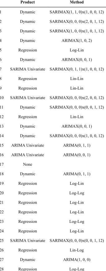
Table A.1: The most acurate model for each product for client 2.

Product Method Model detail

1 Dynamic SARIMAX(1, 1, 0)x(1, 0, 0, 12) 2 Dynamic SARIMAX(0, 0, 0)x(2, 0, 1, 12) 3 Dynamic SARIMAX(1, 0, 0)x(1, 0, 1, 12) 4 Dynamic ARIMAX(1, 0, 2) 5 Regression Log-Lin 6 Dynamic ARIMAX(0, 0, 1) 7 SARIMA Univariate SARIMAX(0, 1, 1)x(1, 0, 0, 12) 8 Regression Lin-Lin

9 Regression Lin-Lin

10 SARIMA Univariate SARIMAX(0, 0, 0)x(2, 0, 0, 12) 11 Dynamic SARIMAX(0, 0, 0)x(0, 0, 1, 12) 12 Regression Lin-Lin

13 Dynamic ARIMAX(0, 0, 1) 14 Dynamic SARIMAX(0, 0, 0)x(1, 0, 0, 12) 15 ARIMA Univariate ARIMA(0, 1, 1) 16 ARIMA Univariate ARIMA(0, 0, 1) 17 None 18 Dynamic ARIMA(0, 1, 1) 19 Regression Log-Lin 20 Regression Log-Log 21 Regression Log-Lin 22 Regression Log-Lin 23 Regression Log-Log 24 Regression Log-Lin

25 SARIMA Univariate SARIMAX(0, 0, 0)x(0, 0, 1, 12) 26 Regression Lin-Log

27 Dynamic ARIMA(1, 0, 0) 28 Regression Log-Log

(29)

29 SARIMA Univariate SARIMAX(0, 0, 0)x(1, 0, 0, 12) 30 None

31 None

32 Dynamic ARIMA(0, 0, 1) 33 Dynamic ARIMA(0, 0, 1) 34 ARIMA Univariate ARIMA(1, 0, 1) 35 None

36 Regression Log-Log 37 Regression Lin-Log 38 None

39 Dynamic ARIMA(1, 1, 1) 40 SARIMA Univariate SARIMAX(0, 0, 0)x(1, 0, 0, 8) 41 Regression Lin-Lin

42 Dynamic ARIMA(0, 1, 1) 43 ARIMA Univariate ARIMA(0, 0, 1) 44 ARIMA Univariate ARIMA(1, 1, 1) 45 Regression Lin-Log 46 Regression Log-Lin 47 Regression Lin-Lin 48 Regression Log-Lin 49 Regression Log-Log 50 Regression Log-Log

51 SARIMA Univariate SARIMAX(0, 0, 0)x(0, 0, 1, 12) 52 Dynamic SARIMAX(0, 0, 0)x(0, 0, 1, 12) 53 None 54 Regression Log-Lin 55 Dynamic ARIMA(0,0,2) 56 Regression Lin-Log 57 Regression Log-Log 58 Regression Log-Lin 59 Dynamic SARIMAX(0, 0, 0)x(1, 0, 0, 12) 60 Dynamic ARIMA(0,0,1) 61 Regression Log-Lin

(30)

62 Dynamic ARIMAX(1, 0, 1) 63 Dynamic ARIMAX(0, 1, 2) 64 SARIMA Univariate SARIMAX(0, 0, 0)x(1, 0, 0, 12) 65 Dynamic ARIMAX(0, 0, 2) 66 Dynamic SARIMAX(0, 1, 1)x(1, 0, 0, 8) 67 Dynamic SARIMAX(0, 0, 0)x(3, 0, 1, 6) 68 Dynamic ARIMAX(0, 1, 1) 69 Dynamic ARIMAX(1, 0, 1) 70 Dynamic ARIMAX(1, 0, 1) 71 ARIMA Univariate ARIMA(0, 1, 1) 72 ARIMA Univariate ARIMA(1, 1, 1) 73 SARIMA Univariate SARIMAX(0, 0, 1)x(0, 0, 1, 12) 74 Regression Log-Log

75 Dynamic ARIMA(0, 1, 1) 76 ARIMA Univariate ARIMA(1, 0, 1) 77 ARIMA Univariate ARIMA(1, 1, 2) 78 Dynamic ARIMA(0, 1, 1) 79 ARIMA Univariate ARIMA(0, 1, 1) 80 ARIMA Univariate ARIMA(1, 1, 1) 81 Dynamic ARIMA(0, 1, 1) 82 Regression Lin-Log 83 ARIMA Univariate ARIMA(0, 1, 1) 84 Dynamic SARIMAX(0, 0, 0)x(1, 0, 1, 12) 85 Dynamic SARIMAX(0, 0, 0)x(1, 0, 0, 12) 86 Dynamic SARIMAX(0, 0, 0)x(1, 0, 0, 12) 87 Dynamic SARIMAX(0, 0, 0)x(1, 0, 0, 12) 88 Dynamic SARIMAX(0, 0, 0)x(2, 0, 0, 12) 89 Dynamic SARIMAX(0, 0, 0)x(1, 0, 1, 12) 90 Dynamic SARIMAX(0, 0, 0)x(2, 0, 0, 12) 91 Dynamic SARIMAX(0, 0, 0)x(2, 0, 0, 12) 92 Dynamic SARIMAX(1, 0, 1)x(2, 0, 0, 12) 93 Dynamic SARIMAX(0, 0, 0)x(1, 0, 1, 12) 94 Dynamic SARIMAX(1, 0, 1)x(2, 0, 0, 12)

(31)

Product Method Model detail 95 Dynamic SARIMAX(0, 0, 0)x(1, 0, 0, 12) 96 Dynamic SARIMAX(1, 0, 0)x(1, 0, 1, 12) 97 Dynamic SARIMAX(0, 0, 0)x(1, 0, 0, 12) 98 Dynamic SARIMAX(0, 0, 0)x(1, 0, 1, 12) 99 Dynamic SARIMAX(0, 0, 0)x(2, 0, 0, 12) 100 Dynamic SARIMAX(0, 0, 0)x(1, 0, 0, 12)

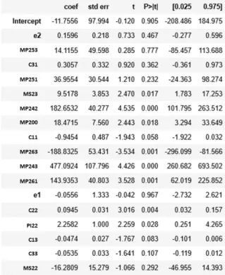
B. Experimental results - Multiple Regression

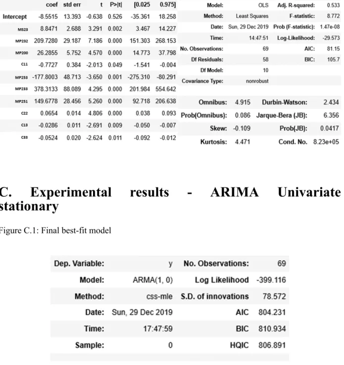
Figure B.1: Best-fit model from transormations and forward selecting strategy

(32)

C. Experimental results - ARIMA Univariate

stationary

Figure C.1: Final best-fit model

D. Experimental results - ARIMA Univariate

non-stationary

(33)

Figure D.1: Final best-fit model

E. Experimental results - Dynamic model

Figure E.1: Final best-fit model

F. Pyhton code

(34)

pip install pmdarima # Data curation import pandas as pd import numpy as np %matplotlib notebook import matplotlib.pyplot as plt import statsmodels.api as sm import statsmodels.formula.api as smf

sales_volume = pd.read_excel('data_clean.xlsx', header=[0,1,2,

3,4], index_col=[0, 1], sheetname='Sales Volume') sales_volume = pd.DataFrame(sales_volume)

sales_volume = sales_volume.replace(np.NaN, 0)

def get_tokens(string): import re

tokens = re.sub(r'[^\sa-zA-Z0-9]', '', string).lower().str ip().split()

return tokens

#Variables definition

y_raw = pd.read_excel('data_clean.xlsx', header=[0,1,2,3,4], i ndex_col=[0, 1], sheetname='Sales Volume')

y_raw = y_raw.replace(np.NaN, 0) y_raw = pd.DataFrame(y_raw)

(35)

x1 = pd.read_excel('data_clean.xlsx', skiprows = 17, header=[0

,1], index_col=[0, 1], sheetname='Internal Data-Promo Intensit y')

x1 = pd.DataFrame(x1)

,1,2], index_col=[0, 1], sheetname='Internal Data-MarketPenetr ation')

,1], index_col=[0, 1], sheetname='Internal Data-Market Share') x3 = pd.DataFrame(x3)

x4 = pd.read_excel('data_clean.xlsx', skiprows = 7, header=[0,

1], index_col=[0, 1], sheetname='Stores per Client') x4 = pd.DataFrame(x4)

x4cleancols1 = pd.DataFrame('x4'+ x4.iloc[:,0:8].columns.get_l evel_values(0) + x4.iloc[:,0:8].columns.get_level_values(1)) x4cleancols2 = get_tokens(str(x4cleancols1))

x4cleancols = [x for x in x4cleancols2 if x.startswith('x4')] x4.columns = x4cleancols

x5 = pd.read_excel('data_clean.xlsx', skiprows = 2, header=[0,

1,2], index_col=[0, 1], sheetname='Internal Data-Media Plan') x5 = x5.replace(np.NaN, 0)

(36)

0,1], index_col=[0, 1], sheetname='External Data') e_n = pd.DataFrame(e_n)

e_n.columns = ['e1', 'e2', 'e3', 'e41', 'e42', 'e43', 'e5']

# Categories

#Y - sales time series:

aftersun_pd = y_raw.iloc[:, 0:4] labello_pd = y_raw.iloc[:, 36:56] bath_pd = y_raw.iloc[:, 57:68] shower_pd = y_raw.iloc[:, 69:100] inshower_pd = y_raw.iloc[:, 146:153] soap_pd = y_raw.iloc[:,101:116]

bodyessentials_pd = y_raw.iloc[:, 117:146] bodyperformance_pd = y_raw.iloc[:,154:166] bodyapc_pd = y_raw.iloc[:,167:181]

facecare_pd = y_raw.iloc[:, 182:244] facecleansing_pd = y_raw.iloc[:,245:289] hand_pd = y_raw.iloc[:,290:302]

deofemale_pd = y_raw.iloc[:, 302:339] deomale_pd = y_raw.iloc[:,340:367] haircare_pd = y_raw.iloc[:, 368:401] styling_pd = y_raw.iloc[:, 402:419] aftershave_pd = y_raw.iloc[:, 420:431] menfacecare_pd = y_raw.iloc[:, 432:465] sunprotect_pd = y_raw.iloc[:,466:514]

(37)

x1facecleansing = x1.iloc[:, 4:8]

x1facecleansingcleancols1 = pd.DataFrame('x1facecleansing'+ x 1facecleansing.columns.get_level_values(1))

x1facecleansingcleancols = get_tokens(str(x1facecleansingclean cols1))

x1facecleansingcleancols = [x for x in x1facecleansingcleancol s if x.startswith('x1')]

logx1facecleansing = np.log(x1.iloc[:, 4:8].replace(0,1))

logx1facecleansingcleancols1 = pd.DataFrame('logx1facecleansi ng'+ x1facecleansing.columns.get_level_values(1))

logx1facecleansingcleancols = get_tokens(str(logx1facecleansin gcleancols1))

logx1facecleansingcleancols = [x for x in logx1facecleansingcl eancols if x.startswith('logx1')]

logx1facecleansing.columns =logx1facecleansingcleancols x1facecleansing.columns = x1facecleansingcleancols

x2face = x2.iloc[:, 0:10]

x2facecleancols1 = pd.DataFrame('x2face'+ x2face.columns.get_ level_values(1)+ x2face.columns.get_level_values(2))

x2facecleancols = get_tokens(str(x2facecleancols1))

x2facecleancols = [x for x in x2facecleancols if x.startswith( 'x2')]

logx2face = np.log(x2.iloc[:, 0:10].replace(0,1))

logx2facecleancols1 = pd.DataFrame('logx2face'+ x2face.column s.get_level_values(1)+ x2face.columns.get_level_values(2)) logx2facecleancols = get_tokens(str(logx2facecleancols1))

logx2facecleancols = [x for x in logx2facecleancols if x.start swith('logx2')]

(38)

logx2face.columns =logx2facecleancols x2face.columns = x2facecleancols

x3facecleansing = x3.iloc[:, 3:6]

x3facecleansingcleancols1 = pd.DataFrame('x3facecleansing'+ x 3facecleansing.columns.get_level_values(1))

x3facecleansingcleancols = get_tokens(str(x3facecleansingclean cols1))

x3facecleansingcleancols = [x for x in x3facecleansingcleancol s if x.startswith('x3')]

logx3facecleansing = np.log(x3.iloc[:, 3:6].replace(0,1))

logx3facecleansingcleancols1 = pd.DataFrame('logx3facecleansi ng'+ x3facecleansing.columns.get_level_values(1))

logx3facecleansingcleancols = get_tokens(str(logx3facecleansin gcleancols1))

logx3facecleansingcleancols = [x for x in logx3facecleansingcl eancols if x.startswith('logx3')]

logx3facecleansing.columns =logx3facecleansingcleancols x3facecleansing.columns = x3facecleansingcleancols

x1facecare = x1.iloc[:, 9:12]

x1facecarecleancols1 = pd.DataFrame('x1facecare'+ x1facecare.

columns.get_level_values(1))

x1facecarecleancols = get_tokens(str(x1facecarecleancols1)) x1facecarecleancols = [x for x in x1facecarecleancols if x.sta rtswith('x1')]

logx1facecare = np.log(x1.iloc[:, 9:12].replace(0,1))

logx1facecarecleancols1 = pd.DataFrame('logx1facecare'+ x1fac ecare.columns.get_level_values(1))

(39)

logx1facecarecleancols = get_tokens(str(logx1facecarecleancols 1))

logx1facecarecleancols = [x for x in logx1facecarecleancols if x.startswith('logx1')]

logx1facecare.columns =logx1facecarecleancols x1facecare.columns = x1facecarecleancols

x3facecare = x3.iloc[:, 6:9]

x3facecarecleancols1 = pd.DataFrame('x3facecare'+ x3facecare.

x3facecarecleancols = get_tokens(str(x3facecarecleancols1)) x3facecarecleancols = [x for x in x3facecarecleancols if x.sta rtswith('x3')]

logx3facecare = np.log(x3.iloc[:, 6:9].replace(0,1))

logx3facecarecleancols1 = pd.DataFrame('logx3facecare'+ x3fac ecare.columns.get_level_values(1))

logx3facecarecleancols = get_tokens(str(logx3facecarecleancols 1))

logx3facecarecleancols = [x for x in logx3facecarecleancols if x.startswith('logx3')]

logx3facecare.columns =logx3facecarecleancols x3facecare.columns = x3facecarecleancols

x1bodyessentials = x1.iloc[:, 16:20]

x1bodyessentialscleancols1 = pd.DataFrame('x1bodyessentials'+

x1bodyessentials.columns.get_level_values(1))

x1bodyessentialscleancols = get_tokens(str(x1bodyessentialscle ancols1))

(40)

ols if x.startswith('x1')]

logx1bodyessentials = np.log(x1.iloc[:, 16:20].replace(0,1)) logx1bodyessentialscleancols1 = pd.DataFrame('logx1bodyessent ials'+ x1bodyessentials.columns.get_level_values(1))

logx1bodyessentialscleancols = get_tokens(str(logx1bodyessenti alscleancols1))

logx1bodyessentialscleancols = [x for x in logx1bodyessentials cleancols if x.startswith('logx1')]

logx1bodyessentials.columns =logx1bodyessentialscleancols x1bodyessentials.columns = x1bodyessentialscleancols

x2body = x2.iloc[:, 10:26]

x2bodycleancols1 = pd.DataFrame('x2body'+ x2body.columns.get_ level_values(1)+ x2body.columns.get_level_values(2))

x2bodycleancols = get_tokens(str(x2bodycleancols1))

x2bodycleancols = [x for x in x2bodycleancols if x.startswith( 'x2')]

logx2body = np.log(x2.iloc[:, 10:26].replace(0,1))

logx2bodycleancols1 = pd.DataFrame('logx2body'+ x2body.column s.get_level_values(1)+ x2body.columns.get_level_values(2)) logx2bodycleancols = get_tokens(str(logx2bodycleancols1))

logx2bodycleancols = [x for x in logx2bodycleancols if x.start swith('logx2')]

logx2body.columns =logx2bodycleancols x2body.columns = x2bodycleancols

x3bodyessentials = x3.iloc[:, 12:15]

x3bodyessentialscleancols1 = pd.DataFrame('x3bodyessentials'+

(41)

x3bodyessentialscleancols = get_tokens(str(x3bodyessentialscle ancols1))

x3bodyessentialscleancols = [x for x in x3bodyessentialscleanc ols if x.startswith('x3')]

logx3bodyessentials = np.log(x3.iloc[:, 12:15].replace(0,1)) logx3bodyessentialscleancols1 = pd.DataFrame('logx3bodyessent ials'+ x3bodyessentials.columns.get_level_values(1))

logx3bodyessentialscleancols = get_tokens(str(logx3bodyessenti alscleancols1))

logx3bodyessentialscleancols = [x for x in logx3bodyessentials cleancols if x.startswith('logx3')]

logx3bodyessentials.columns =logx3bodyessentialscleancols x3bodyessentials.columns = x3bodyessentialscleancols

x1bodyperformance = x1.iloc[:, 20:24]

x1bodyperformancecleancols1 = pd.DataFrame('x1bodyperformanc e'+ x1bodyperformance.columns.get_level_values(1))

x1bodyperformancecleancols = get_tokens(str(x1bodyperformancec leancols1))

x1bodyperformancecleancols = [x for x in x1bodyperformanceclea ncols if x.startswith('x1')]

logx1bodyperformance = np.log(x1.iloc[:, 20:24].replace(0,1)) logx1bodyperformancecleancols1 = pd.DataFrame('logx1bodyperfo rmance'+ x1bodyperformance.columns.get_level_values(1))

logx1bodyperformancecleancols = get_tokens(str(logx1bodyperfor mancecleancols1))

logx1bodyperformancecleancols = [x for x in logx1bodyperforman cecleancols if x.startswith('logx1')]

(42)

x1bodyperformance.columns = x1bodyperformancecleancols

x3bodyperformance = x3.iloc[:, 15:18]

x3bodyperformancecleancols1 = pd.DataFrame('x3bodyperformanc e'+ x3bodyperformance.columns.get_level_values(1))

x3bodyperformancecleancols = get_tokens(str(x3bodyperformancec leancols1))

x3bodyperformancecleancols = [x for x in x3bodyperformanceclea ncols if x.startswith('x3')]

logx3bodyperformance = np.log(x3.iloc[:, 15:18].replace(0,1)) logx3bodyperformancecleancols1 = pd.DataFrame('logx3bodyperfo rmance'+ x3bodyperformance.columns.get_level_values(1))

logx3bodyperformancecleancols = get_tokens(str(logx3bodyperfor mancecleancols1))

logx3bodyperformancecleancols = [x for x in logx3bodyperforman cecleancols if x.startswith('logx3')]

logx3bodyperformance.columns =logx3bodyperformancecleancols x3bodyperformance.columns = x3bodyperformancecleancols

x1bodyapc = x1.iloc[:, 24:28]

x1bodyapccleancols1 = pd.DataFrame('x1bodyapc'+ x1bodyapc.col umns.get_level_values(1))

x1bodyapccleancols = get_tokens(str(x1bodyapccleancols1))

x1bodyapccleancols = [x for x in x1bodyapccleancols if x.start swith('x1')]

logx1bodyapc = np.log(x1.iloc[:, 24:28].replace(0,1))

logx1bodyapccleancols1 = pd.DataFrame('logx1bodyapc'+ x1bodya pc.columns.get_level_values(1))

(43)

))

logx1bodyapccleancols = [x for x in logx1bodyapccleancols if x

.startswith('logx1')]

logx1bodyapc.columns =logx1bodyapccleancols x1bodyapc.columns = x1bodyapccleancols

x3bodyapc = x3.iloc[:, 18:21]

x3bodyapccleancols1 = pd.DataFrame('x3bodyapc'+ x3bodyapc.col umns.get_level_values(1))

x3bodyapccleancols = get_tokens(str(x3bodyapccleancols1))

x3bodyapccleancols = [x for x in x3bodyapccleancols if x.start swith('x3')]

logx3bodyapc = np.log(x3.iloc[:, 18:21].replace(0,1))

logx3bodyapccleancols1 = pd.DataFrame('logx3bodyapc'+ x3bodya pc.columns.get_level_values(1))

logx3bodyapccleancols = get_tokens(str(logx3bodyapccleancols1 ))

logx3bodyapccleancols = [x for x in logx3bodyapccleancols if x

logx3bodyapc.columns =logx3bodyapccleancols x3bodyapc.columns = x3bodyapccleancols

x1shower = x1.iloc[:, 28:32]

x1showercleancols1 = pd.DataFrame('x1shower'+ x1shower.column s.get_level_values(1))

x1showercleancols = get_tokens(str(x1showercleancols1))

x1showercleancols = [x for x in x1showercleancols if x.startsw ith('x1')]

(44)

logx1showercleancols1 = pd.DataFrame('logx1shower'+ x1shower.

logx1showercleancols = get_tokens(str(logx1showercleancols1)) logx1showercleancols = [x for x in logx1showercleancols if x.s tartswith('logx1')]

logx1shower.columns =logx1showercleancols x1shower.columns = x1showercleancols

x2showercleancols1 = pd.DataFrame('x2shower'+ x2shower.column s.get_level_values(1)+ x2shower.columns.get_level_values(2)) x2showercleancols = get_tokens(str(x2showercleancols1))

x2showercleancols = [x for x in x2showercleancols if x.startsw ith('x2')]

logx2shower = np.log(x2.iloc[:, 45:58].replace(0,1))

columns.get_level_values(1)+ x2shower.columns.get_level_values (2))

x3showercleancols1 = pd.DataFrame('x3shower'+ x3shower.column s.get_level_values(1))

x3showercleancols = get_tokens(str(x3showercleancols1))

(45)

ith('x3')]

logx3shower = np.log(x3.iloc[:, 21:24].replace(0,1))

x1deofemale = x1.iloc[:, 37:41]

x1deofemalecleancols1 = pd.DataFrame('x1deofemale'+ x1deofema le.columns.get_level_values(1))

x1deofemalecleancols = get_tokens(str(x1deofemalecleancols1)) x1deofemalecleancols = [x for x in x1deofemalecleancols if x.s tartswith('x1')]

logx1deofemale = np.log(x1.iloc[:, 37:41].replace(0,1))

logx1deofemalecleancols1 = pd.DataFrame('logx1deofemale'+ x1d eofemale.columns.get_level_values(1))

logx1deofemalecleancols = get_tokens(str(logx1deofemalecleanco ls1))

logx1deofemalecleancols = [x for x in logx1deofemalecleancols if x.startswith('logx1')]

logx1deofemale.columns =logx1deofemalecleancols x1deofemale.columns = x1deofemalecleancols

x2deo = x2.iloc[:, 27:46]

x2deocleancols1 = pd.DataFrame('x2deo'+ x2deo.columns.get_lev el_values(1)+ x2deo.columns.get_level_values(2))

(46)

x2deocleancols = get_tokens(str(x2deocleancols1))

x2deocleancols = [x for x in x2deocleancols if x.startswith('x 2')]

logx2deo = np.log(x2.iloc[:, 27:46].replace(0,1))

logx2deocleancols1 = pd.DataFrame('logx2deo'+ x2deo.columns.g et_level_values(1)+ x2deo.columns.get_level_values(2))

logx2deocleancols = get_tokens(str(logx2deocleancols1))

logx2deocleancols = [x for x in logx2deocleancols if x.startsw ith('logx2')]

logx2deo.columns =logx2deocleancols x2deo.columns = x2deocleancols

x3deofemale = x3.iloc[:, 28:31]

x3deofemalecleancols1 = pd.DataFrame('x3deofemale'+ x3deofema le.columns.get_level_values(1))

x3deofemalecleancols = get_tokens(str(x3deofemalecleancols1)) x3deofemalecleancols = [x for x in x3deofemalecleancols if x.s tartswith('x3')]

logx3deofemale = np.log(x3.iloc[:, 28:31].replace(0,1))

logx3deofemalecleancols1 = pd.DataFrame('logx3deofemale'+ x3d eofemale.columns.get_level_values(1))

logx3deofemalecleancols = get_tokens(str(logx3deofemalecleanco ls1))

logx3deofemalecleancols = [x for x in logx3deofemalecleancols if x.startswith('logx3')]

logx3deofemale.columns =logx3deofemalecleancols x3deofemale.columns = x3deofemalecleancols

(47)

x1deomalecleancols1 = pd.DataFrame('x1deomale'+ x1deomale.col umns.get_level_values(1))

x1deomalecleancols = get_tokens(str(x1deomalecleancols1))

x1deomalecleancols = [x for x in x1deomalecleancols if x.start swith('x1')]

logx1deomale = np.log(x1.iloc[:, 40:44].replace(0,1))

logx1deomalecleancols1 = pd.DataFrame('logx1deomale'+ x1deoma le.columns.get_level_values(1))

logx1deomalecleancols = get_tokens(str(logx1deomalecleancols1 ))

logx1deomalecleancols = [x for x in logx1deomalecleancols if x

logx1deomale.columns =logx1deomalecleancols x1deomale.columns = x1deomalecleancols

x3deomale = x3.iloc[:, 30:33]

x3deomalecleancols1 = pd.DataFrame('x3deomale'+ x3deomale.col umns.get_level_values(1))

x3deomalecleancols = get_tokens(str(x3deomalecleancols1))

x3deomalecleancols = [x for x in x3deomalecleancols if x.start swith('x3')]

logx3deomale = np.log(x3.iloc[:, 30:33].replace(0,1))

logx3deomalecleancols1 = pd.DataFrame('logx3deomale'+ x3deoma le.columns.get_level_values(1))

logx3deomalecleancols = get_tokens(str(logx3deomalecleancols1 ))

logx3deomalecleancols = [x for x in logx3deomalecleancols if x

(48)

x3deomale.columns = x3deomalecleancols

x1menaftershave = x1.iloc[:, 48:52]

x1menaftershavecleancols1 = pd.DataFrame('x1menaftershave'+ x 1menaftershave.columns.get_level_values(1))

x1menaftershavecleancols = get_tokens(str(x1menaftershaveclean cols1))

x1menaftershavecleancols = [x for x in x1menaftershavecleancol s if x.startswith('x1')]

logx1menaftershave = np.log(x1.iloc[:, 48:52].replace(0,1)) logx1menaftershavecleancols1 = pd.DataFrame('logx1menaftersha ve'+ x1menaftershave.columns.get_level_values(1))

logx1menaftershavecleancols = get_tokens(str(logx1menaftershav ecleancols1))

logx1menaftershavecleancols = [x for x in logx1menaftershavecl eancols if x.startswith('logx1')]

logx1menaftershave.columns =logx1menaftershavecleancols x1menaftershave.columns = x1menaftershavecleancols

x2menaftershavecleancols1 = pd.DataFrame('x2menaftershave'+ x 2menaftershave.columns.get_level_values(1)+ x2menaftershave.co lumns.get_level_values(2))

logx2menaftershave = np.log(x2.iloc[:, 87:103].replace(0,1)) logx2menaftershavecleancols1 = pd.DataFrame('logx2menaftersha

(49)

ve'+ x2menaftershave.columns.get_level_values(1)+ x2menaftersh ave.columns.get_level_values(2))

x3menaftershavecleancols1 = pd.DataFrame('x3menaftershave'+ x 3menaftershave.columns.get_level_values(1))

logx3menaftershave = np.log(x3.iloc[:, 36:39].replace(0,1)) logx3menaftershavecleancols1 = pd.DataFrame('logx3menaftersha ve'+ x3menaftershave.columns.get_level_values(1))

x1menfacecare = x1.iloc[:, 52:56]

x1menfacecarecleancols1 = pd.DataFrame('x1menfacecare'+ x1men facecare.columns.get_level_values(1))

(50)

x1menfacecarecleancols = get_tokens(str(x1menfacecarecleancols 1))

x1menfacecarecleancols = [x for x in x1menfacecarecleancols if x.startswith('x1')]

logx1menfacecare = np.log(x1.iloc[:, 52:56].replace(0,1))

logx1menfacecarecleancols1 = pd.DataFrame('logx1menfacecare'+

x1menfacecare.columns.get_level_values(1))

logx1menfacecarecleancols = get_tokens(str(logx1menfacecarecle ancols1))

logx1menfacecarecleancols = [x for x in logx1menfacecarecleanc ols if x.startswith('logx1')]

logx1menfacecare.columns =logx1menfacecarecleancols x1menfacecare.columns = x1menfacecarecleancols

x2menfacecarecleancols1 = pd.DataFrame('x2menfacecare'+ x2men facecare.columns.get_level_values(1)+ x2menfacecare.columns.ge t_level_values(2))

logx2menfacecare = np.log(x2.iloc[:, 103:113].replace(0,1)) logx2menfacecarecleancols1 = pd.DataFrame('logx2menfacecare'+

x2menfacecare.columns.get_level_values(1)+ x2menfacecare.colum ns.get_level_values(2))

(51)

ols if x.startswith('logx2')]

x3menfacecarecleancols1 = pd.DataFrame('x3menfacecare'+ x3men facecare.columns.get_level_values(1))

logx3menfacecare = np.log(x3.iloc[:, 39:42].replace(0,1))

logx3menfacecarecleancols1 = pd.DataFrame('logx3menfacecare'+

x3menfacecare.columns.get_level_values(1))

logx3menfacecarecleancols = [x for x in logx3menfacecarecleanc ols if x.startswith('logx3')]

x1sunprotection = x1.iloc[:, 60:64]

x1sunprotectioncleancols1 = pd.DataFrame('x1sunprotection'+ x 1sunprotection.columns.get_level_values(1))

x1sunprotectioncleancols = get_tokens(str(x1sunprotectionclean cols1))

x1sunprotectioncleancols = [x for x in x1sunprotectioncleancol s if x.startswith('x1')]

(52)

logx1sunprotectioncleancols1 = pd.DataFrame('logx1sunprotecti on'+ x1sunprotection.columns.get_level_values(1))

logx1sunprotectioncleancols = get_tokens(str(logx1sunprotectio ncleancols1))

logx1sunprotectioncleancols = [x for x in logx1sunprotectioncl eancols if x.startswith('logx1')]

logx1sunprotection.columns =logx1sunprotectioncleancols x1sunprotection.columns = x1sunprotectioncleancols

x2sun = x2.iloc[:, 113:126]

x2suncleancols1 = pd.DataFrame('x2sun'+ x2sun.columns.get_lev el_values(1)+ x2sun.columns.get_level_values(2))

x2suncleancols = get_tokens(str(x2suncleancols1))

x2suncleancols = [x for x in x2suncleancols if x.startswith('x 2')]

logx2sun = np.log(x2.iloc[:, 113:126].replace(0,1))

logx2suncleancols1 = pd.DataFrame('logx2sun'+ x2sun.columns.g et_level_values(1)+ x2sun.columns.get_level_values(2))

logx2suncleancols = get_tokens(str(logx2suncleancols1))

logx2suncleancols = [x for x in logx2suncleancols if x.startsw ith('logx2')]

logx2sun.columns =logx2suncleancols x2sun.columns = x2suncleancols

x3sunprotection = x3.iloc[:, 45:48]

x3sunprotectioncleancols1 = pd.DataFrame('x3sunprotection'+ x 3sunprotection.columns.get_level_values(1))

x3sunprotectioncleancols = get_tokens(str(x3sunprotectionclean cols1))

(53)

x3sunprotectioncleancols = [x for x in x3sunprotectioncleancol s if x.startswith('x3')]

logx3sunprotection = np.log(x3.iloc[:, 45:48].replace(0,1)) logx3sunprotectioncleancols1 = pd.DataFrame('logx3sunprotecti on'+ x3sunprotection.columns.get_level_values(1))

logx3sunprotectioncleancols = get_tokens(str(logx3sunprotectio ncleancols1))

logx3sunprotectioncleancols = [x for x in logx3sunprotectioncl eancols if x.startswith('logx3')]

logx3sunprotection.columns =logx3sunprotectioncleancols x3sunprotection.columns = x3sunprotectioncleancols

x1sunaftersun = x1.iloc[:, 64:68]

x1sunaftersuncleancols1 = pd.DataFrame('x1sunaftersun'+ x1sun aftersun.columns.get_level_values(1))

x1sunaftersuncleancols = get_tokens(str(x1sunaftersuncleancols 1))

x1sunaftersuncleancols = [x for x in x1sunaftersuncleancols if x.startswith('x1')]

logx1sunaftersun = np.log(x1.iloc[:, 64:68].replace(0,1))

logx1sunaftersuncleancols1 = pd.DataFrame('logx1sunaftersun'+

x1sunaftersun.columns.get_level_values(1))

logx1sunaftersuncleancols = get_tokens(str(logx1sunaftersuncle ancols1))

logx1sunaftersuncleancols = [x for x in logx1sunaftersuncleanc ols if x.startswith('logx1')]

logx1sunaftersun.columns =logx1sunaftersuncleancols x1sunaftersun.columns = x1sunaftersuncleancols

(54)

x3sunaftersun = x3.iloc[:, 48:51]

x3sunaftersuncleancols1 = pd.DataFrame('x3sunaftersun'+ x3sun aftersun.columns.get_level_values(1))

x3sunaftersuncleancols = get_tokens(str(x3sunaftersuncleancols 1))

x3sunaftersuncleancols = [x for x in x3sunaftersuncleancols if x.startswith('x3')]

logx3sunaftersun = np.log(x3.iloc[:, 48:51].replace(0,1))

logx3sunaftersuncleancols1 = pd.DataFrame('logx3sunaftersun'+

x3sunaftersun.columns.get_level_values(1))

logx3sunaftersuncleancols = get_tokens(str(logx3sunaftersuncle ancols1))

logx3sunaftersuncleancols = [x for x in logx3sunaftersuncleanc ols if x.startswith('logx3')]

logx3sunaftersun.columns =logx3sunaftersuncleancols x3sunaftersun.columns = x3sunaftersuncleancols

x1lipcare = x1.iloc[:, 68:72]

x1lipcarecleancols1 = pd.DataFrame('x1lipcare'+ x1lipcare.col umns.get_level_values(1))

x1lipcarecleancols = get_tokens(str(x1lipcarecleancols1))

x1lipcarecleancols = [x for x in x1lipcarecleancols if x.start swith('x1')]

logx1lipcare = np.log(x1.iloc[:, 68:72].replace(0,1))

logx1lipcarecleancols1 = pd.DataFrame('logx1lipcare'+ x1lipca re.columns.get_level_values(1))

logx1lipcarecleancols = get_tokens(str(logx1lipcarecleancols1 ))