Diversity and Distributions, (Diversity Distrib.) (2005) 11, 477– 486
B I O D I V E R S I T Y
R E S E A R C H
ABSTRACT
Bonelli’s eagle, Hieraaetus fasciatus, has recently suffered a severe population decline and is currently endangered. Spain supports about 70% of the European population. We used stepwise logistic regression on a set of environmental, spatial and human variables to model Bonelli’s eagle distribution in the 5167 UTM 10 × 10 km quadrats of peninsular Spain. We obtained a model based on 16 variables, which allowed us to identify favourable and unfavourable areas for this species in Spain, as well as inter-mediate favourability areas. We assessed the stepwise progression of the model by comparing the model’s predictions in each step with those of the final model, and selected a parsimonious explanatory model based on three variables — slope, July temperature and precipitation — comprising 76% of the predictive capacity of the final model. The reported presences in favourable and unfavourable areas suggest a source–sink dynamics in Bonelli’s eagle populations. The fragmented spatial structure of the favourable areas suggests the existence of a superimposed metapopulation dynamics. Previous LIFE (The Financial Instrument of the European Union for the Environment and Nature) projects for the conservation of this species have focused mainly on the northern limit of its range, where the sharpest population decline has been recorded. In these areas, favourability is low and Bonelli’s eagle populations are probably maintained by the immigration of juveniles produced in more favourable zones. However, southern populations, although stable, show signs of reduction in productivity, which could menace the population sizes in the whole study area. We suggest that conservation efforts should focus also on known favourable areas, which might favour population persistence in unfavourable areas through dispersal. Keywords
Endangered species, favourable areas, LIFE projects, metapopulation, predictive and explanatory models, source–sink dynamics.
INTRODUCTION
The knowledge of species distributions patterns and the identifi-cation of factors influencing these patterns are crucial for managing biodiversity (e.g. Krebs, 1978; Brown, 1984). In recent years, the modelling of species distributions has been increasingly used to identify suitable habitat and to predict potential distributions (e.g. Austin, 2002; Williams & Araújo, 2002; Robertson et al., 2003; Rushton et al., 2004). The development of relatively simple species distribution models is particularly interesting in the case
of endangered species (Donázar et al., 1993). Understanding
where and why species occur is a necessary precursor for schemes to mitigate population decline and to create new populations through reintroduction (Rushton et al., 2004).
Bonelli’s eagle, Hieraaetus fasciatus (Vieillot 1822), is a
widespread raptor whose western Palaearctic populations are
distributed mainly in the Mediterranean area, generally in fairly
warm and dry regions (Del Hoyo et al., 1994). In recent decades,
this species has suffered one of the most severe population declines recorded among birds of prey, and has been listed as an endangered European species (Rocamora, 1994; BirdLife Inter-national/EBCC, 2000). In Spain, which with 650 –713 breeding pairs (Real, 2003) supports about 70% of the European population, the species has recently changed its status from vulnerable (IUCN categories, Blanco & González, 1992) to endangered (IUCN categories; Madroño et al., 2004), and high-priority conservation has been urged (De Juana, 1992). European (Council Directive 79/409/EEC) and Spanish (Real Decreto 439/1990) legislations include it as a priority target species for special conservation
measures. Real & Mañosa (1997) and Carrete et al. (2002a)
reported, for the 1980–97 period, local extinction rates ranging from 32.1% to 48.6% in different Spanish localities.
Laboratory of Biogeography, Diversity and Conservation. Department of Animal Biology, Faculty of Sciences, University of Malaga, E-29071 Malaga, Spain
*Correspondence: A. Román Muñoz, Department of Information and Computer Sciences, Nara Women’s University, Kita-Uoya Nishimachi, Nara 630-8506, Japan.
Tel: +81 0742 203983. Fax: +81 0742 203983 E-mail: [email protected]
Present address: Department of Information and Computer Sciences, Nara Women’s University, Kita-Uoya Nishimachi, Nara 630-8506, Japan Blackwell Publishing, Ltd.
Modelling the distribution of Bonelli’s
eagle in Spain: implications for
conservation planning
A. R. Muñoz et al.
Investigation on the factors that affect Bonelli’s eagle has been mostly based on local-scale ecological studies (e.g. Gil-Sánchez
et al., 1996; Rico et al., 1999; Carrete et al., 2002a; Ontiveros
et al., 2005). The main reported causes of the decline are direct
persecution, and electrocution by and collision with electric
power lines (Carrete et al., 2002b; Real, 2003), which seriously
affect the adult survival rate. However, Bonelli’s eagle popula-tions are not only affected by local habitat characteristics, but also by historical, environmental and human-related processes that act on larger geographical scales (Ricklefs, 1987; Levin, 1992). These large-scale processes may be related to the complex transient behaviour common in many spatially extended popu-lations (Hastings & Higgins, 1994; White & Bowers, 1996), which may give place to metapopulation (Levins, 1970) or source–sink (Pulliam, 1988) dynamics. Coulson et al. (2001) and Stenseth et al. (2002), for instance, associated large-scale climatic indices with many species population dynamics. Consequently, broad-scale distribution models may help conservation programs to attain more satisfactory results, as the factors that affect the popula-tions on a larger scale are taken into account (Corsi et al., 1999;
Lehmann et al., 2002). Predictive distribution models, although
may fail, have important potential applications: they can forecast species occurrence in poorly documented areas, predict the response of species to changes in environmental conditions, or reveal adequate target areas for species reintroduction or conservation programmes (Fielding & Haworth, 1995).
The recently published atlas of Spanish breeding birds (Martí & del Moral, 2003) provided comprehensive large-scale distribution data of Bonelli’s eagle, so allowing a wider view on its distribution and the performing of analyses that take greater parts of its range into account.
The aim of this study was to model the distribution of Bonelli’s eagle in peninsular Spain to predict the potential distribution of this species and to identify favourable and unfavourable areas. The implications of the obtained models are analysed in order to assess the possible success of future conservation plans for this endangered species.
METHODS Study area
Peninsular Spain covers an area of 493,518 km2, and includes
important mountain ranges that reach a maximum altitude of 3478 m. The climate is heterogeneous, with a mainly eastward- and southward-decreasing gradient of precipitation and a mainly northward-decreasing gradient of temperature (Font, 2000). Spain may be divided into three climatic areas: Atlantic, Mediterranean and Interior. The Atlantic area is characterized by mild winters and cool summers, and by abundant and regular precipitation. The Mediterranean part experiences hot summers and mild winters; rainfall rarely exceeds 500 mm annually and occurs mainly during spring and autumn. In the Interior part, the temperatures are high in summer and low in winter, and precipitation is irregular and scarce (Capel, 1981).
Distribution data and statistical analyses
Bonelli’s eagle presence or absence data on 5167 UTM 10 × 10 km
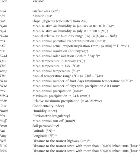
of peninsular Spain were obtained from the atlas of Spanish breeding birds (Martí & del Moral, 2003). As the distribution data shown in the atlas were slightly displaced for protection reasons, we obtained the original presence and absence data from the Spanish Ministry for the Environment. Bonelli’s eagle is present in 817 peninsular Spanish UTM grid cells. We used 29 independent variables related to spatial situation, topography, climate, lithology and human activity to model Bonelli’s eagle distribution in peninsular Spain (Table 1).
We digitized the variables (except for Alti, which was made
available as a digital coverage by the Land Processes Distributed Active Archive Center, located at the US Geological Survey’s
EROS Data Center, http://LPDAAC.usgs.gov) using the
1.2 software and processed them using the 32 software.
Isoline variables (HJan through Long) were interpolated from a
triangulated irregular network performing parabolic bridge and
tunnel edge removal. Area was calculated using the 32
AREA module. Secondary variables, defined in Table 1 by an algebraic operation in parentheses, were calculated from primary variables using the Idrisi Image Calculator. Distance variables (DHi, U100 and U500) were calculated from the digitized
high-ways and urban centres using the DISTANCE module. The
resolution scale adopted for all variables was 1 pixel c. 1 km2. We
then extracted the mean values of the variables for each UTM
10 × 10 km of peninsular Spain (n = 5167) using a digital UTM
grid map provided by the Área de Defensa Contra Incendios
Forestales (DGCN, Ministerio de Medio Ambiente, Spain). Perm
was obtained from a map of synthesis of ground-water aquifers, a categorical map with three different permeability classes (I.G.M.E.,
1979). We determined Perm for each UTM 10 × 10 km by
calcu-lating the average of the values assigned to the pixels within the square.
To predict the potential distribution of Bonelli’s eagle in Spain, we performed a stepwise logistic regression (Hosmer & Lemeshow, 1989) of the eagle’s presence/absence data on these variables. When the number of presences and absences within the territory is different, as here, the probability values yielded by logistic regression are biased toward the category with the great-est number of cases. To overcome this, we eliminated the random probability element, which is ln(presences/absences), from the regression logit equation, so that a value of 0.5 corresponded to a neutral environmental favourability value, that is, the environ-mental conditions that yield the same probability of occurrence as expected at random. In this way, corrected probability values strictly reflect habitat or biogeographical favourability for the species. We used the corrected 0.5 value as a threshold to classify the squares as expected presences and absences, and assessed the sensitivity and the specificity of the model (see, for example, Brito et al., 1999).
However, as Hosmer & Lemeshow (1989) pointed out, it makes little sense to establish as markedly different areas with, for example, 0.48 and 0.52 favourability values. Consequently, we opted for opening a gap between the values considered as clearly
Biogeography and conservation of Bonelli’s eagle in Spain
favourable and clearly unfavourable. We classified each UTM
10 × 10 km into three categories, depending on their
favour-ability values. If the predicted favourfavour-ability was higher than 0.8, which means that the odds are more than 4:1 favourable to the species, the square was considered as favourable. Areas with a favourability value lower than 0.2 (odds less than 1:4) were considered unfavourable to the species. The remaining squares were considered as intermediate favourability areas.
We also assessed the evolution of the model as the selected variables were added by checking the correlation of the favourabil-ity values obtained in each step with those of the final predictive model. We parsimoniously explained the model in terms of the variables included in the step that significantly explained more than 75% (R2 > 0.75) of the final model, and considered these
variables to be the explanatory variables. To take into account interactions between these factors, which often result in an overlaid effect in space due to colinearity between them (Borcard
et al., 1992; Legendre, 1993), we performed a variation
partition-ing procedure to specify how much of the variation of the final model was explained by the pure effect of each explanatory variable, which proportion was attributable to their interaction,
and how these variables interact affecting the target variable (Legendre, 1993; Legendre & Legendre, 1998).
The part of the variation of the final model explained by each explanatory variable ( ) was obtained by performing logistic regression of Bonelli’s eagle presence/absence data on each explanatory variable, and regressing the values obtained in the final model on those yielded by the models based on each variable. The amount of variation explained by each pair, trio, etc. of
explanatory variables ( ) may be obtained by regressing
the final model values on those yielded by the logistic regression model using these variables. Then, the pure effect of each variable
( ) may be assessed by subtracting the variation explained by
the other variables together from the variation explained by all
explanatory variables together ( ). The
variation attributable to the interaction of pairs of variables ( )
may be obtained by subtracting from the pure effect of
the two variables ( ) and the variation explained by the
other variables together ( ). The variation attributable to
interactions among trios, quartets, etc. may be obtained analo-gously by subtraction (see Legendre & Legendre, 1998, pp. 532– 534; Whittaker, 1984).
Code Variable
Area Surface area (km2)
Alti Altitude (m)*
Slop Slope (degrees) (calculated from Alti)
HJan Mean relative air humidity in January at 07 : 00 h (%)† HJul Mean relative air humidity in July at 07 : 00 h (%)† HRan Annual relative air humidity range (%) (= |HJan – HJul|) PET Mean annual potential evapotranspiration (mm)†
AET Mean annual actual evapotranspiration (mm) (= min[PET, Prec]) Inso Mean annual insolation (hours/year)†
SRad Mean annual solar radiation (kwh m−2 day−1)† TJan Mean temperature in January (°C)† TJul Mean temperature in July (°C)† Temp Mean annual temperature (°C)†
TRan Annual temperature range (°C) (= TJul – TJan)
DFro Mean annual number of frost days (minimum temperature ≤ 0 °C)† DPre Mean annual number of days with precipitation ≥ 0.1 mm† Prec Mean annual precipitation (mm)†
MP24 Maximum precipitation in 24 h (mm)† RMP Relative maximum precipitation (= MP24/Prec)
Cont Continentality index‡
Humi Humidity index‡
PIrr Pluviometric irregularity§
ROff Mean annual run-off (mm)¶
Perm Soil permeability¶
Lati Latitude (°N)**
Long Longitude (°E)**
DHi Distance to the nearest highway (km)**
U100 Distance to the nearest town with more than 100,000 inhabitants (km)** U500 Distance to the nearest town with more than 500,000 inhabitants (km)**
Sources of data: *US Geological Survey (1996). †Font (1983). ‡Font (2000). §Montero de Burgos & González-Rebollar (1974). ¶I.G.M.E. (1979). **I.G.N. (1999); data on the number of inhabitants of urban centres taken from the Instituto Nacional de Estadística (<http://www.ine.es>).
Table 1 Variables used to model the determinants of distribution of Bonelli’s eagle (Hieraaetus fasciatus) in peninsular Spain Ri 2 Ri j+ + +...n 2 RPi 2 RPi Ri j n Rj n 2 2 2 = + + +... − + +... Rij 2 Ri j+ + +...n 2 RPi RPj 2 2 + Rk+ +...n 2
A. R. Muñoz et al.
RESULTS
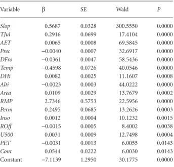
Table 2 shows the variables included in the model and their coefficients in the logit function, ranked according to their order of entrance in the model.
Favourability values for Bonelli’s eagle in the peninsular Spanish UTM grid cells are represented in Fig. 1.
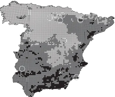
The favourability classes for the UTM 10 × 10 km are shown
in Fig. 2. There are 2109 unfavourable squares, and only in 31 (1.5%) of these squares is the species present. Regarding favour-able squares, 336 out of the 529 (63.5%) have been reported to support eagles. The intermediate favourability area comprises 2529 squares of which 450 (17.8%) support the species.
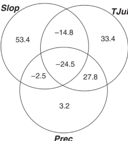
Figure 3 shows the stepwise evolution of the model, and the squared correlation between the favourabilities predicted in each step and those of the final model, that is, the proportion of variance of the final model accounted for by each step. About 83% of the predictive capacity of the final model is reached in the fourth step, which points out the high capacity of this partial model to predict the distribution of the species using only four variables. Table 3 shows the correct classification rates for pres-ences and abspres-ences (see Hosmer & Lemeshow, 1989, p. 146) in the squares for the partial model in the fourth step and for the final model. However, step 3 did not increase the explanatory power of step 2, so we only included Slope, TJul and Prec in our parsimonious explanatory model. These three variables explained 76% of the variation in the final model values. The results of the final model variation partitioning are shown in Fig. 4.
DISCUSSION
The explanatory model
The distribution of Bonelli’s eagle is well described by a limited number of topographical, climatic and human-related variables. Although the good fit of a model does not necessarily imply correct inference of causation (James & McCulloch, 1990), our parsimonious explanatory model suggested that the suitable areas for this species are mountainous with a Mediterranean
Table 2 Variables included in the model and their coefficients (β), standard errors (SE), Wald test values (Wald, 1943) and significance (P). The variables are ranked according to their order of entrance in the model. Variables codes as in Table 1
Variable β SE Wald P Slop 0.5687 0.0328 300.5550 0.0000 TJul 0.2916 0.0699 17.4104 0.0000 AET 0.0065 0.0008 69.5845 0.0000 Prec −0.0040 0.0007 32.6917 0.0000 DFro −0.0361 0.0047 58.5436 0.0000 Temp −0.4598 0.0726 40.0546 0.0000 DHi 0.0082 0.0025 11.1607 0.0008 Alti −0.0023 0.0003 44.0222 0.0000 Area 0.0109 0.0029 13.7679 0.0002 RMP 2.7346 0.5753 22.5956 0.0000 Perm 0.2495 0.0685 13.2626 0.0003 Inso 0.0012 0.0004 10.1232 0.0015 ROff −0.0015 0.0005 8.4002 0.0038 U500 0.0031 0.0009 12.7498 0.0004 PET −0.0031 0.0013 6.0055 0.0143 Cont 0.0544 0.0222 6.0030 0.0143 Constant −7.1139 1.2950 30.1775 0.0000
Figure 1 Favourability values for Bonelli’s eagle in each UTM 10 × 10 km square of peninsular Spain, shown on a scale ranging from 0 (white) to 1 (black).
Biogeography and conservation of Bonelli’s eagle in Spain
climate characterized by hot summers and low precipitation. This confirms the previously described dependence of the species on warm and dry conditions and sunny mountains (Cramp & Simmons, 1980; Del Hoyo et al., 1994).
Mean slope is probably related with cliff availability, the most limiting resource for the breeding of this cliff-nesting eagle. Although it can also breed on trees, less than 1.7% of the Spanish population do it (Arroyo et al., 1995). Sánchez-Zapata et al. (1996) found that those territories with steepest cliffs tended to remain occupied during periods of population decline. Since nest orientation is also important for the species, being the productivity higher in nests orientated toward the south-east (Ontiveros, 1999; Ontiveros & Pleguezuelos, 2003a), a greater cliff availability increases eagle-nesting options.
Mean slope alone explains only 11.6% of the final model (Fig. 3). However, the pure effect of slope on the final model is more than 53% (Fig. 4), which seems to indicate that the true role of slope only is apparent after taking also into account TJul and Prec. Cartron et al. (2000) pointed out that when in a system with three variables, two correlations are positive and one negative, the expected relationships may not all be observed following a bivariate approach. This is the case with Slop, TJul and the final model, as the models based on each of these variables correlate positively with the final model but negatively between them
(RSlop-TJul = −0.318). The same occurs with Slop and Prec
(RSlop-Prec = −0.482). In this way, the effect of Slop is obscured by
both TJul and Prec, and vice versa, in the amount expressed by the negative interactions shown in Fig. 4. The combined pure effect of TJul and Prec explains 64.4% of the final model (see Fig. 4), which may be considered the effect attributable to Mediterranean climate independently of slope. In other words, Bonelli’s eagle selects mountainous areas with Mediterranean
climate, but mountainous areas tend to be segregated from Mediterranean areas, so their true effect only is really shown when both factors are considered together.
Ontiveros and Pleguezuelos (2003b) found that average annual temperature is the main climatic variable explaining the breeding success of Bonelli’s eagle throughout its latitudinal range in the western Mediterranean. Parellada et al. (1984) and Gil-Sánchez et al. (1996) also noted the influence of temperature on the distribution of the species in Spain at a local scale. Our results suggest that this species prefers areas with hot summers, which is somehow puzzling, as protection from thermal extremes is an important factor in nest site selection for medium- and large-sized raptors (Collias & Collias, 1984). However, Bonelli’s eagle is the earliest breeder among all Mediterranean eagles (Cramp & Simmons, 1980), so it could prefer areas with very hot summers because they are detrimental to competitors, whereas it would be able to dodge the effect of high summer temperatures by breeding early.
The role of human activity
Human activity may have a secondary role in Bonelli’s eagle distribution. The species presence is more likely as the distance to
Figure 2 Favourability classes for Bonelli’s eagle in the UTM 10 × 10 km of peninsular Spain. Black squares represent odds more than 4:1 favourable to the presence of the species, white squares represent odds more than 4:1 unfavourable to the species and grey squares represent intermediate favourability areas. The circles enclose the areas object of LIFE conservation projects for Bonelli’s eagle.
Table 3 Correct classification rates achieved by the model on step 4 and on the last step of the logistic regression procedure (n = 5167)
Presences (n = 817) Absences (n = 4350) Total Step 4 81.5% 75.1% 76.1% Step 22 84.1% 75.3% 76.7%
A. R. Muñoz et al.
highways and to big cities increases. This does not necessarily imply active or passive killing of eagles by humans. These variables could be seen as large-scale surrogates for disturbance (e.g. Maurer, 1996), as proximity to highways and big cities means higher human density and economic activity, higher interference in the landscape and, in general, a higher level of human disturbance.
Bonelli’s eagle can tolerate a certain degree of human presence (Gil-Sánchez et al., 1996; Carrete et al., 2002a) and its tolerance to human proximity is higher than that of other cliff-nesting raptors. However, Real & Mañosa (1997) and Mañosa & Real (2001) pointed out that habitat destruction, direct persecution, decline in prey availability, disturbance at nesting sites, electro-cution and collision with transmission lines, all of them derived from human activity, are the main causes of its population decline. In southern Spain, territories closer to the source of
potential human disturbance are usually occupied by non-adult eagles (Balbontín et al., 2003), which could indicate that these tend to be suboptimal areas for the species.
Source–sink and metapopulation dynamics
The existence of favourable and unfavourable areas suggests that source–sink dynamics (Pulliam, 1988) could be implicated in the distribution of the species. If populations may show different demographic rates depending on the favourability of the occupied habitat (e.g. Weiss et al., 1988; Kadmon, 1993; Ferrer & Donázar, 1996), then favourable areas could act as net exporters of eagles to unfavourable territories. These dispersers are juveniles and immatures, which form an important fraction of the total population, since Bonelli’s eagle, as other long-living birds of
Figure 3 Favourability maps predicted by the model in each intermediate step of the logistic regression procedure, and squared Pearson’s correlation coefficients between them and the favourabilities predicted by the final model.
Biogeography and conservation of Bonelli’s eagle in Spain
prey, delays the acquisition of sexual maturity for several years (Newton, 1979). A high proportion of these young Bonelli’s eagles travel long distances, up to 1020 km (Real & Mañosa, 2001). Because of this, Carrete et al. (2002b) proposed that management of local populations of this species should take into account not only local events but also the dispersal of young individuals over a wider area. This could be particularly true for unfavourable areas and, to a lesser extent, for areas of intermediate favourability, whose populations could be maintained by the immigration of juveniles mainly produced in favourable areas.
However, if the reproductive surplus in favourable habitats would be large enough to compensate the reproductive deficit in unfavourable ones, then a significant part of the population would be expected to exist in unsuitable habitats (Pulliam, 1996). According to our model only 1.5% of unfavourable squares support Bonelli’s eagles, which suggests that a weakening of the source–sink dynamics is occurring.
Juvenile dispersal movements may allow the eagles to explore and settle not only in suboptimal unfavourable areas, but also in unoccupied optimal areas (Horn, 1983), thus facilitating the connection between different favourable habitats. The fragmented spatial structure of the favourable areas in our distribution model suggests the existence of a metapopulation dynamics (Levins, 1969; Hanski & Simberloff, 1997; Carrete et al., 2005) superimposed to the source–sink dynamics. In this situation, if the availability of unoccupied favourable territories is low, then a source–sink dynamics prevails, as juveniles are forced to occupy less favourable territories. Conversely, an increase in unoccupied favourable territories might promote a metapopulation dynamics, which would be detrimental to the source-sink dynamics, so causing a population decline in sink areas. As the availability of unoccupied optimal territories depends mainly on adult mortality, this could be the key factor in the balance between the two types of spatial dynamics. In favourable areas, an increase in adult mortality would not result in an in situ population decline, as
adults would be replaced by subadults, but a rejuvenation of the population would be expected.
Balbontín et al. (2003) detected an increase in the percentage of pairs with at least one non-adult during the period 1980–2000 in the Andalusian population, considered to be one of the last strongholds of this species in Europe. As the productivity of this kind of pairs is lower, this may also result in a reduction in overall productivity (Balbontín et al., 2003), which would diminish the availability of new juveniles in the whole studied area (but see Gil-Sánchez et al., 2005).
The sharpest population decline of Bonelli’s eagle in Spain has been observed in the northern limit of its range (e.g. Real & Mañosa, 1997), where low favourability values are reached, whereas southern and southeastern populations remain stable (Balbontín et al., 2003; Gil-Sánchez et al., 2004). This led to pay attention to the characteristics of northern areas, when the conditions of other, more favourable areas could also explain this decline if the populations acting as a source failed to export enough emigrants.
Our results show that the complex internal structure of geo-graphical distributions, here measured in terms of favourability, plays a critical role on patterns of range contraction and abun-dance decline. Though the demographical (Brown, 1995, p. 216) and contagion (Channell & Lomolino, 2000a,b) hypotheses are alternative explanations, our results are more in accordance with those of Rodríguez (2002), who found that North American birds tended to decline in areas of high abundance, which are not necessarily at the centre of their distribution range. We may add that even when a decline is noticed in low-abundance areas, the cause may actually be acting in those of high abundance. If this process is a major mechanism driving range contractions and large-scale declines in abundance, as Rodríguez (2002) argued, then favourable areas would be those of greater conservation value, particularly for early detection and prevention of population declines.
Bonelli’s eagle has benefited from LIFE projects for its conser-vation. From January 1997 to June 2006, an amount of nearly
$8 million will have been invested on this species (<http://
europa.eu.int/comm/environment/life/home.htm>), co-financed by the European Union (68.7% of the budget) and the Spanish Government. These projects are generally focused on the unfavourable areas where a huge decline has been recorded (see Fig. 2). For example, project LIFE02 NAT/E/008598, which is being developed in Important Bird Areas within the province of Burgos (northern Spain), concentrates its effort on a population that comprised 17 pairs in 1989 and only seven in 2000. We agree that any action within the Bonelli’s eagle range directed to preserve its habitat and to avoid the drastic fall of the species is necessary, but we suggest that the auspicious status of the species in southern favourable areas could be deceptive. We could be facing a rarefaction wave of the species, from northwest to southeast, already noticeable at the limits of its range, in sink or unfavourable areas, although the cause could be located in source areas. We suggest that actions favoured through LIFE projects in unfavourable areas should be complemented with actions in favourable areas, which might favour population persistence in unfavourable areas through dispersal processes.
Figure 4 Results of the variation partitioning of the final model
using the explanatory variables. Abbreviations of variable names are listed in Table 1. Values shown in the diagrams are the percentages of variation explained by the indicated variables and by their interactions. Unexplained variation of the final model is
= 0.24. Runexplained
A. R. Muñoz et al.
ACKNOWLEDGEMENTS
A. Román Muñoz’s research is financed by a grant (ICB2-CT-2002–80007) from the European Commission Research Directo-rate, and A. Márcia Barbosa’s by a doctoral grant (SFRH/BD/ 4601/2001) from the Fundação para a Ciência e a Tecnologia, Portugal. Cosme Morillo (Dirección General de Conservación de la Naturaleza-Ministerio de Medio Ambiente) and Juan Carlos del Moral (SEO/BirdLife) provided the digital atlas data. Dave Richardson, Jon Paul Rodríguez and an anonymous referee provided thoughtful comments and constructive criticism on the manuscript.
REFERENCES
Arroyo, B., Ferreiro, E. & Garza, V. (1995) El Águila Perdicera
( Hieraaetus Fasciatus) en España. Censo, reproducción y conservación. Colección Técnica. ICONA, Madrid.
Austin, M.P. (2002) Spatial prediction of species distribution: an interface between ecological theory and statistical modelling.
Ecological Modelling, 157, 101–118.
Balbontín, J., Penteriani, V. & Ferrer, M. (2003) Variations in the age of mates as an early warning signal of changes in popula-tion trends? The case of Bonelli’s eagle in Andalusia. Biological
Conservation, 109, 417– 423.
BirdLife International /EBCC. (2000) European bird populations:
estimates and trends. BirdLife International (BirdLife
Conser-vation Series no. 10), Cambridge, UK.
Blanco, J.C. & González, J.L. (1992) Libro rojo de los vertebrados
de España. Colección Técnica. ICONA, Madrid.
Borcard, D., Legendre, P. & Drapeau, P. (1992) Partialling out the spatial component of ecological variation. Ecology, 73, 1045–1055. Brito, J.C., Crespo, E.G. & Paulo, O.S. (1999) Modelling wildlife distributions: logistic multiple regression vs overlap analysis.
Ecography, 22, 251–260.
Brown, J.H. (1984) On the relationship between distribution and abundance. American Naturalist, 124, 255–279.
Brown, J.H. (1995) Macroecology. The University of Chicago Press, Chicago.
Capel, J.J. (1981) Los climas de España. Oikos-Tau SA Ediciones, Barcelona.
Carrete, M., Sánchez-Zapata, J.A., Martínez, J.E., Sánchez, M.A. & Calvo, J.F. (2002a) Factors influencing the decline of a Bonelli’s eagle Hieraaetus fasciatus population in southeastern Spain: demography, habitat or competition? Biodiversity and
Conservation, 11, 975–985.
Carrete, M., Sánchez-Zapata, J.A., Martínez, J.E. & Calvo, J.F. (2002b) Predicting the implications of conservation manage-ment: a territorial occupancy model of Bonelli’s eagle in Murcia, Spain. Oryx, 36, 349–356.
Carrete, M., Sánchez-Zapata, J.A., Calvo, J.F. & Lande, R. (2005) Demography and habitat availability in territorial occupancy of two competing species. Oikos, 108, 125–136.
Cartron, J.-L.E., Kelly, J.F. & Brown, J.H. (2000) Constraints on patterns of covariation: a case study in strigid owls. Oikos, 90, 381–389.
Channell, R. & Lomolino, M.V. (2000a) Dynamic biogeography and the conservation of endangered species. Nature, 403, 84–86. Channell, R. & Lomolino, M.V. (2000b) Trajectories to extinc-tion: spatial dynamics of the contraction of geographical ranges. Journal of Biogeography, 27, 169–179.
Collias, N.E. & Collias, E.C. (1984) Nest building and bird
beha-viour. Princeton University Press, Princeton, NJ.
Corsi, F., Duprè, E. & Boitani, L. (1999) A large-scale model of wolf distribution in Italy for conservation planning.
Conservation Biology, 13, 150–159.
Coulson, T., Catchpole, E.A., Albon, S.D., Morgan, B.J.T., Pemberton, J.M., Clutton-Brock, T.H., Crawley, M.J. & Grenfell, B.T. (2001) Age, sex, density, winter weather, and population crashes in Soay sheep. Science, 292, 1528–1531. Cramp, S. & Simmons, K.E.L. (1980) The birds of the western
palearctic, Vol. II. Oxford University Press, Oxford.
De Juana, E. (1992) Algunas prioridades en la conservación de aves en España. Ardeola, 39, 73–84.
Del Hoyo, J., Elliot, A. & Sargatal, J. (1994) Handbook of the birds
of the world, Vol. II. New world vultures to guineafowl. Lynx
Edicions, Barcelona.
Donázar, J.A., Hiraldo, F. & Bustamante, J. (1993) Factors influencing nest site selection, breeding density and breeding success in the Bearded Vulture (Gypaetus barbatus). Journal of
Applied Ecology, 30, 504–514.
Ferrer, M. & Donázar, J.A. (1996) Density-dependent fecundity by habitat heterogeneity in an increasing population of Spanish Imperial Eagles. Ecology, 77, 69–74.
Fielding, A.H. & Haworth, P.F. (1995) Testing the generality of bird-habitat models. Conservation Biology, 9, 1466–1481. Font, I. (1983) Atlas climático de España. Instituto Nacional de
Meteorología, Madrid.
Font, I. (2000) Climatología de España y Portugal. Ediciones Universidad de Salamanca, Salamanca.
Gil-Sánchez, J.M., Molino, F. & Valenzuela, G. (1996) Selección de hábitat de nidificación por el Águila Perdicera (Hieraaetus
fasciatus) en Granada (SE de España). Ardeola, 43, 189–197.
Gil-Sánchez, J.M., Moleón, M., Otero, M. & Bautista, J. (2004) A nine-year study of successful breeding in a Bonelli’s eagle population in southeast Spain: a basis for conservation.
Biological Conservation, 118, 685–694.
Gil-Sánchez, J.M., Moleón, M., Bautista, J. & Otero, M. (2005) Differential composition in the age of mates in Bonelli’s eagle populations: the role of spatial scale, non-natural mortality reduction, and the age classes definition. Biological
Conserva-tion, 124, 149–152.
Hanski, I. & Simberloff, D. (1997) The metapopulation approach, its history, conceptual domain, and application to conservation. Metapopulation biology: ecology, genetics and
evolution (ed. by I. Hanski and M. Gilpin), pp. 5–26. Academic
Press, San Diego.
Hastings, A. & Higgins, K. (1994) Persistence of transients in spatially structured models. Science, 263, 1133–1136.
Horn, H.S. (1983) Some theories about dispersal. The ecology of
animal movement (ed. by R. Swingland and P.J. Greenwood),
Biogeography and conservation of Bonelli’s eagle in Spain Hosmer, D.W., Jr & Lemeshow, S. (1989) Applied logistic
regres-sion. John Wiley & Sons, New York.
I.G.M.E. (1979) Mapa hidrogeológico nacional. Explicación de los
mapas de lluvia útil, de reconocimiento hidrogeológico y de síntesis de los sistemas acuíferos 2nd edn. Instituto Geológico y
Minero de España, Madrid.
I.G.N. (1999) Mapa de carreteras. Península Ibérica, Baleares y
Canarias. Instituto Geográfico Nacional /Ministerio de
Fomento, Madrid.
James, F.C. & McCulloch, C.E. (1990) Multivariate analysis in ecology and systematics: panacea or Pandora’s box? Annual
Review of Ecology and Systematics, 21, 129–166.
Kadmon, R. (1993) Population dynamics consequences of habitat heterogeneity: an experimental study. Ecology, 74, 816–825. Krebs, C.J. (1978) The experimental analysis of distribution and
abundance. Harper & Row, New York.
Legendre, P. (1993) Spatial autocorrelation: trouble or new paradigm? Ecology, 74, 1659–1673.
Legendre, P. & Legendre, L. (1998) Numerical ecology. Second
English edition. Elsevier Science, Amsterdam.
Lehmann, A., Leathwick, J.R. & Overton, J.McC. (2002) Assessing New Zealand fern diversity from spatial predictions of species assemblages. Biodiversity and Conservation, 11, 2217–2238. Levin, S.A. (1992) The problem of pattern and scale in ecology.
Ecology, 73, 1943–1967.
Levins, R. (1969) Some demographic and genetic consequences of environmental heterogeneity for biological control. Bulletin
of the Entomological Society of America, 15, 237–240.
Levins, R. (1970) Extinction. Lecture notes in mathematical life
sciences, 2, 75–107.
Madroño, A., González, C. & Atienza, J.C. (2004) Libro Rojo de
las Aves de España. Ministerio de Medio Ambiente-Sociedad
Española de Ornitología, Madrid.
Mañosa, S. & Real, J. (2001) Potential negative effects of colli-sions with transmission lines on a Bonelli’s Eagle population.
Journal of Raptor Research, 35, 247–252.
Martí, R. & del Moral, J.C. (2003) Atlas de las aves reproductoras
de España. Ministerio de Medio Ambiente-Sociedad Española
de Ornitología, Madrid.
Maurer, B.A. (1996) Relating human population growth to the loss of biodiversity. Biodiversity Letters, 3, 1–5.
Montero de Burgos, J.L. & González-Rebollar, J.L. (1974)
Diagramas bioclimáticos. ICONA, Madrid.
Newton, I. (1979) Population ecology of raptors. T & AD Poyser, UK.
Ontiveros, D. (1999) Selection of nest cliffs by Bonelli’s eagle (Hieraaetus fasciatus) in southeastern Spain. Journal of Raptor
Research, 33, 110–116.
Ontiveros, D. & Pleguezuelos, J.M. (2003a) Physical, environ-mental and human factors influencing productivity in Bonelli’s eagle Hieraaetus fasciatus in Granada (SE Spain).
Biodiversity and Conservation, 12, 1193–1203.
Ontiveros, D. & Pleguezuelos, J.M. (2003b) Influence of climate on Bonelli’s eagle’s (Hieraaetus fasciatus V, 1822) breeding success through the western Mediterranean. Journal of
Bio-geography, 30, 755–760.
Ontiveros, D., Pleguezuelos, J.M. & Caro, J. (2005) Prey density, prey detectability and food habits: the case of Bonelli’s eagle and the conservation measures. Biological Conservation, 123, 19–25.
Parellada, X., De Juan, A. & Alamany, O. (1984) Ecologia de l’aliga cuabarrada (Hieraaetus fasciatus): factors limitants, adaptacions morfológiques i ecológiques i relacions interespecífiques amb l’aliga daurada (Aquila chrysaetos).
Rapinyaires Mediterranis, 2, 121–141.
Pulliam, H.R. (1988) Sources, sinks and population regulation.
American Naturalist, 132, 652–661.
Pulliam, H.R. (1996) Sources and sinks: empirical evidence and population consequences. Population dynamics in ecological
space and time (ed. by O.E. Rhodes, R.K. Chesser and
M.H. Smith), pp. 45–69. University of Chicago Press, Chicago. Real, J. (2003) Águila-azor Perdicera, Hieraaetus fasciatus. Atlas
de las Aves Reproductoras de España. (ed. by R. Marti and
J.C. del Moral), pp. 192–193. Ministerio de Medio Ambiente-Sociedad Española de Ornitología, Madrid.
Real, J. & Mañosa, S. (1997) Demography and conservation of Western European Bonelli’s Eagle (Hieraaetus fasciatus) populations. Biological Conservation, 79, 59–66.
Real, J. & Mañosa, S. (2001) Dispersal oj juvenile and inmature Bonelli’s Eagles in northeastern Spain. Journal of Raptor
Research, 35, 9–14.
Ricklefs, R.E. (1987) Community diversity: relative roles of local and regional processes. Science, 235, 167–171.
Rico, L., Sánchez-Zapata, J.A., Izquierdo, A., García, J.R., Morán, S. & Rico, D. (1999) Tendencias recientes en las poblaciones del Águila Real Aquila chrysaetos y el Águila-azor Perdicera
Hieraaetus fasciatus en la provincia de Valencia. Ardeola, 46,
235–238.
Robertson, M.P., Peter, C.I., Villet, M.H. & Ripley, B.S. (2003) Comparing models for predicting species’ potential distribu-tions: a case study using correlative and mechanistic predictive modelling techniques. Ecological Modelling, 164, 153–167. Rocamora, G. (1994) Bonelli’s Eagle Hieraaetus fasciatus. Birds
in Europe, their conservation status (ed. by G.M. Tucker and
M.F. Heath), pp. 184–185. BirdLife International (BirdLife Conservation Series no. 3), Cambridge, UK.
Rodríguez, J.P. (2002) Range contraction in declining North American bird populations. Ecological Applications, 12, 238– 248.
Rushton, S.P., Ormerod, S.J. & Kerby, G. (2004) New paradigms for modelling species distributions? Journal of Applied Ecology,
41, 193–200.
Sánchez-Zapata, J.A., Sánchez, M.A., Calvo, J.F., González, G. & Martínez, J.E. (1996) Selección de hábitat de las aves de presa en la región de Murcia (SE de España). Biology and
conserva-tion of mediterranean raptors, 1994 (ed. by J. Muntaner and
J. Mayol), pp. 299 –304. SEO/BirdLife Monografías no. 4, Madrid. Stenseth, N.C., Mysterud, A., Ottersen, G., Hurrell, J.W.,
Chan, K.-S. & Lima, M. (2002) Ecological effects of climate fluctuations. Science, 297, 1292–1296.
US Geological Survey (1996) GTOPO30. Land Processes Distributed Active Archive Center (LP DAAC), EROS Data
A. R. Muñoz et al.
Center, http://edcdaac.usgs.gov/gtopo30/gtopo30.asp. Cited 22 September 1999.
Wald, A. (1943) Tests of statistical hypotheses concerning several parameters with applications to problems of estimation.
Trans-actions of the American Mathematical Society, 54, 426–482.
Weiss, S.B., Murph, D.D. & White, R.R. (1988) Sun, slope and butterflies: topographic determinants of habitat quality for
Euphydryas editha. Ecology, 69, 1486–1496.
White, J.A. & Bowers, R.F. (1996) Host-pathogen systems in a
spatially patchy environment. Proceedings of the Royal Society
of London. Series B, Biological Sciences, 263, 325–332.
Whittaker, J. (1984) Model interpretation from the additive elements of the likelihood function. Applied Statistics, 33, 52–64.
Williams, P.H. & Araújo, M.B. (2002) Apples, oranges, and probabilities: integrating multiple factors into biodiversity conservation with consistency. Environmental Modeling and