F
ACULDADE DEE
NGENHARIA DAU
NIVERSIDADE DOP
ORTODetection and Characterization of
Defects in Composite Materials Using
Thermography
António José Ramos da Silva
Programa Doutoral em Engenharia Mecânica Supervisor: Prof. Dr. Joaquim Gabriel Magalhães Mendes
Supervisor: Prof. Dr. Mário Augusto Pires Vaz
Abstract
Composite materials are widely used in the transport industry, particularly aeronautics, due to their light weight and enhanced mechanical properties. On the downside, these new materials are less known and their behaviour are unpredictable greatly because of their anisotropic properties, being difficult to simulate and understand their behaviour. To overcome these aspects regular preventive maintenance operations are necessary.
In order to avoid major problems, Non-Destructive Testing (NDT) are a solution to assure the safety without destroying the components. From the vast possibilities available, field image NDT have proved to be fast, precise and easy to interpret. Image technologies usually capture and measure some type of electromagnetic radiation to identify a discontinuity in the radiation pattern that changes due to a component abnormality. Since the natural radiation emitted by objects at the ambient temperature is in the infrared waveband, this is used to create a temperature image, particularly in the middle and far-infrared wavebands. Better results can be obtained when is used a stimulation source to induce a temperature variation, highlighting any defect that a component may have. Two different types of tests can be done with: single or periodic stimulation. When using single stimulation (transient tests), a pulse of energy is applied to the object and observed its recovery to the previous equilibrium state. On the other hand, when performing periodic tests (lock-in), the stimulation is modulated in several cycles, with the amplitude response and phase delay being analysed.
This work aimed to develop a numeric model able to predict the result of an infrared thermal test in carbon fiber reinforced polymers with structural defects. This work is divided in three main parts: field tests, numeric simulation and model validation. Several different field tests were performed with various test samples to identify the settings that produced the best results and give the highest sensitivity to defects detection. These tests were performed using the above refereed techniques, transient and lock-in. During the lock-in tests, it was identified an imperfection in the modulated sinusoidal stimulation, which was quantified and corrected improving the overall results.
The samples used in the laboratory testes where simulated using the finite element technique in Matlab R. This manner it was obtained an internal view of the heat flow inside the component
and provided the temperature evolution at the surface of the specimen during an entire test. With the results obtained from the simulations, it is possible to estimate the thermal response obtained with a certain type of test and waveform.
Finally, the model was validated with experimental tests, consisting of samples made of carbon fiber reinforced polymers poly-methyl-meth-acrylate. At the end of this document it is presented a short comparison between the two thermal techniques and shearography.
Resumo
Os materiais compósitos são cada vez mais utilizados em diversas indústrias. A indústria dos transportes, em particular aeronáutica, procura tirar partido de materiais que sejam mais resistentes e leves. Os materiais compósitos possuem propriedades menos conhecidas e o seu comportamento é mais difíceis de modelar. Uma vez que eles são normalmente anisotrópicos são ainda mais imprevisíveis e difíceis de simular. Para contornar estas dificuldades são executadas regularmente operações de manutenção preventiva.
De forma a evitar graves problemas, devem ser utilizados ensaios não destrutivos, garantindo um bom desempenho sem por em causa a integridade do componente. Das diversas técnicas existentes as técnicas de imagem têm-se mostrado rápidas, precisas e fáceis de interpretar. As técnicas de imagem captam e medem uma parte do espectro eletromagnético para identificar uma descontinuidade ou alteração no padrão de radiação alterado devido a um defeito no componente. Uma vez que a radiação emitida pelos objetos à temperatura ambiente está no campo da radiação infravermelha, particularmente infravermelhos médios e os longos, esta é utilizada para criar imagens de temperatura. Os melhores resultados são obtidos quando é utilizada uma fonte de estimulação para induzir uma alteração na temperatura, realçando possíveis defeitos. Estes testes podem ser divididos em duas categorias: estimulação singular ou periódicas. Nos testes com estimulação transiente, esta é aplicada de uma forma uniforme durante um período de tempo e é analisada a evolução da temperatura. Contudo, quando são utilizadas estimulações cíclicas lock-in, a estimulação é modulada em vários ciclos e calculada a amplitude e atraso de resposta.
O trabalho pretendia desenvolver um modelo numérico capaz de prever os resultados de ensaios de termografia ativa em componentes de fibra de carbono com defeitos internos. Este trabalho está dividido em três partes: testes laboratoriais, simulações numéricas e validação do modelo. Foram realizados diversos ensaios laboratoriais, com diversas amostras, de forma a identificar as configurações onde eram obtidos os melhores resultados. Estes testes utilizaram as já referidas técnicas de termografia transient e lock-in. Foi identificada uma imperfeição nas ondas modeladas nos ensaios do tipo lock-in, esta foi quantificada e corrigida, melhorando assim a sensibilidade destes ensaios.
As amostras utilizadas nos ensaios laboratoriais foram simuladas utilizando o método dos elementos finitos, com implementação em Matlab R. Desta forma foi obtida uma visão do fluxo
de calor no interior das amostras e obtidos os perfis térmicos na superfície da amostra durante o teste. Com os resultados obtidos com as simulações é possível estimar a resposta térmica obtida com um determinado tipo de teste e tipo de onda.
Finalmente os modelos desenvolvidos foram validados com ensaios laboratoriais em amostras de textitpoly-methyl-meth-acrylate e fibra de carbono. No final deste documento é apresentada uma breve comparação entre as técnicas de termografia e xerografia.
Acknowledgments
I would like to thank my supervisors, Prof. Dr. Joaquim Gabriel Magalhães Mendes and Prof. Dr. Mário Augusto Pires Vaz, their support and supervision was of the foremost importance. Either by their extensive knowledge in sensors and instrumentation, as for the experience in the field of non-destructive testing, their contribute for this work was essential.
An important contribution was also given by Dr. Pedro Miguel Guimarães Pires Moreira and Dr. Paulo José da Silva Tavares in the comprehension of the fatigue models and simulations. Despite the fact this was not the main subject of this work, it presented an important role in the understanding of the temperature behaviour during cyclic loading. Alongside these, contributions from other members from the Laboratory of Optics and Experimental Mechanics, INEGI, were also very important. To them, I would also like to leave here a note of gratitude.
I would also like to express my gratitude to my laboratory partners, for their suggestions and support that helped me to achieve my goals.
I would like to thank Porto Biomechanics Laboratory (LABIOMEP) from the University of Porto for the thermal camera used to conduct the laboratory tests.
The support of my family was extremely important, without which this work would not be possible. To them I express here my deepest appreciation. To finish, I would like to thank my friends and co-workers. Although I no longer keep daily contact with some of them, during the last years their help, support and understanding was extremely important.
António José Ramos Silva
“The aim [of education] must be the training of independently acting and thinking individuals who, however see in the service to the community their highest life problem.” Albert Einstein 1936.
to Marco Silva my apologies...
Contents
Abstract i Resumo iii 1 Introduction 1 1.1 Context . . . 1 1.2 Main Goal . . . 2 1.3 Structure . . . 22 State of the Art 5 2.1 Composite materials . . . 6
2.1.1 Ceramic matrix composites . . . 7
2.1.2 Metal matrix composites . . . 7
2.1.3 Polymeric matrix composites - resins . . . 8
2.1.4 Polymeric matrix composites - fibres . . . 10
2.1.5 Nanotubes and mechanical properties overview . . . 12
2.2 Non-destructive testing . . . 14 2.2.1 Visual inspections . . . 15 2.2.2 Dye inspection . . . 17 2.2.3 Electromagnetic testing . . . 19 2.2.4 Radiographic testing . . . 20 2.2.5 Acoustic emission . . . 21 2.2.6 Laser testing . . . 23 2.2.7 Vibration analysis . . . 24 2.2.8 Ultrasound testing . . . 25 2.3 Conclusion . . . 28
3 Infrared Thermography and Thermal Tests 29 3.1 Infrared thermography . . . 30
3.1.1 Temperature measurements . . . 30
3.1.2 Infrared thermography principles . . . 31
3.1.3 Infrared thermography measuring parameters . . . 33
3.1.4 Thermography in NDT applications . . . 39
3.1.5 Stimulation sources for IRNDT . . . 40
3.2 Transient thermal testing . . . 47
3.2.1 Overview . . . 47
3.2.2 Experimental setup . . . 48
3.2.3 Experimental protocol . . . 49
3.2.4 Data processing . . . 50
3.2.5 Results . . . 52
3.2.6 Transient Thermal Tests conclusion . . . 59
3.3 Lock-in thermal testing . . . 61
3.3.1 Overview . . . 61
3.3.2 Procedure and processing . . . 62
3.3.3 Results . . . 65
3.3.4 Analyses of lock-in thermal tests . . . 71
3.3.5 Lock-in conclusion . . . 75
3.4 Conclusion . . . 76
4 New Lock-in Thermal Tests 77 4.1 Stimulus characterization . . . 78
4.1.1 Laboratory tests setup . . . 78
4.1.2 Stimulation dynamic characterization . . . 80
4.1.3 Stimulation with PID controller . . . 82
4.1.4 Stimulation response analyses . . . 84
4.2 Feedback modulated tests . . . 86
4.2.1 Setup and settings . . . 86
4.2.2 Results of thermal tests with feedback . . . 86
4.2.3 Feedback tests analyses . . . 89
4.3 Stimulation with PID controller . . . 91
4.3.1 Setup and PID settings . . . 91
4.3.2 Temperature results . . . 92
4.4 Comparison . . . 93
4.4.1 Comparison results . . . 94
4.4.2 Comparison analyses . . . 97
4.5 Conclusions . . . 100
5 Thermal Tests Simulation 101 5.1 Mathematical models . . . 102
5.1.1 System governing equations . . . 102
5.1.2 Finite element method . . . 104
5.1.3 Adopted mesh . . . 106
5.1.4 Evaluating mesh settings . . . 107
5.2 Transient test simulation . . . 111
5.2.1 Introduction to the simulation . . . 111
5.2.2 Results . . . 113
5.2.3 Simulation analyses . . . 118
5.2.4 Optimum settings . . . 122
5.3 Lock-in test simulation . . . 125
5.3.1 Introduction to the simulation . . . 125
5.3.2 Results . . . 127
5.3.3 Simulation analyses . . . 136
5.3.4 Optimum settings . . . 143
CONTENTS xi
6 Optimum Stimulus Validation 149
6.1 Transient test validation . . . 150
6.1.1 Analyses of a sample made of PMMA . . . 150
6.1.2 Analyses of a sample made of CFRP . . . 151
6.2 Lock-in test validation . . . 152
6.2.1 Analyses of a sample made of PMMA . . . 152
6.2.2 Analyses of a sample made of CFRP . . . 155
6.2.3 Results eliminating optical reflection . . . 157
6.3 Comparison with shearography . . . 161
6.4 Conclusion . . . 163
7 Conclusions 165 7.1 Contributions . . . 168
7.2 Future works . . . 169
A Thermal Stress Analyses 171 A.1 Thermal stress testing . . . 171
A.1.1 Overview . . . 171
A.1.2 Experimental protocol . . . 173
A.1.3 Results . . . 176
A.1.4 Analyses . . . 180
A.1.5 TSA conclusions . . . 182
B Equations to Predict Thermal Differences 183 B.1 Transient thermal tests . . . 183
B.1.1 Equations of TTT for PMMA . . . 184
B.1.2 Equations of TTT for CFRP . . . 184
B.2 Lock-in thermal tests . . . 185
B.2.1 Equations of LTT for PMMA . . . 185
B.2.2 Equations of LTT for CFRP . . . 186
C Technical drawings 189 C.1 PMMA with 10 mm slots . . . 189
C.2 CFRP sample . . . 189
C.3 CT sample . . . 189
List of Figures
2.1 Symmetric and asymmetric particle movement . . . 26
3.1 Planck’s law for six different temperatures . . . 32
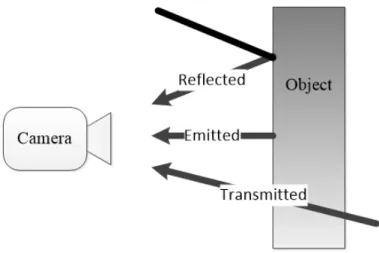
3.2 Different sources of radiation that reach the thermal camera . . . 34
3.3 Temperature variation for different emissivities . . . 35
3.4 Temperature variation for different reflected temperatures . . . 36
3.5 Radiation in the infrared waveband . . . 37
3.6 Detection of corrosion (red line) underneath the painting of an aluminium plate [145] . . . 42
3.7 Detection of dis-bound (red delimitation) in square honeycomb composite [146] . 43 3.8 Detection of a defect in CFRP with microwave stimulation [149] . . . 44
3.9 Detection of a defect in CFRP with ultrasound stimulation [150] . . . 45
3.10 Stress in an aluminium sheet at the tip of a crack . . . 46
3.11 Correlation between type of thermal test, stimulation, and possible analyses . . . 47
3.12 Laboratory tests setup and sample section view . . . 49
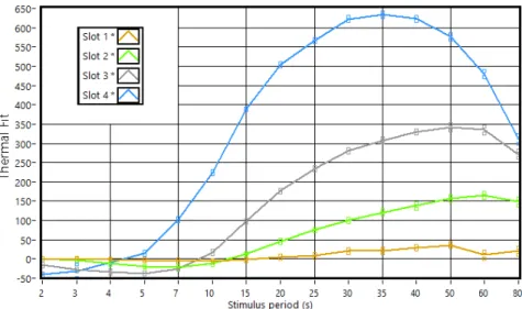
3.13 Example of thermal (12.5 millimetres width) image and measurement locations . 51 3.14 Temperature response for several stimulus durations for samples with different widths . . . 53
3.15 Difference between the temperatures and the adjacent reference temperatures for the plate with the 12.5 mm slots . . . 54
3.16 Slot’s temperature for different stimulation durations, slots with 7.5 millimetres . 57 3.17 Slot width comparison for the 30 seconds stimulation period and image index 350 58 3.18 Comparison of the different types of analyses . . . 59
3.19 Images for the plate with 7.5 millimetres slots, stimulation of 15 seconds and image index 350 . . . 60
3.20 Example of an image from the analyses of a sample with 12.5 millimetres (phase) 64 3.21 Vertical profiles of figure3.20 . . . 64
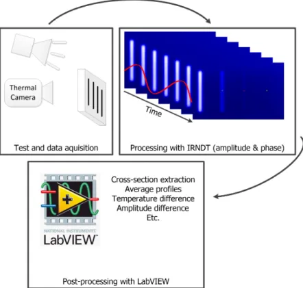
3.22 Schematic of the steps performed in a lock-in test. . . 65
3.23 Normalized phase and amplitude response . . . 66
3.24 Comparison of the two interpolation methods, harmonic and DFT . . . 67
3.25 Average phase cross-section profiles . . . 67
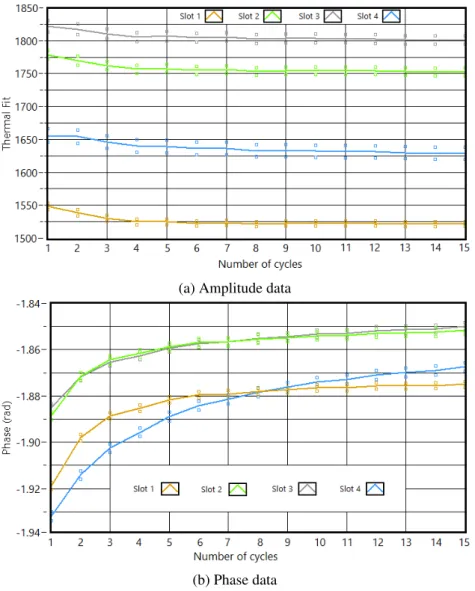
3.26 Variation of the slots data for several number of cycles in the stimulation . . . 68
3.27 Average amplitude and phase cross-sections . . . 70
3.28 Results for slots with different width and depths . . . 71
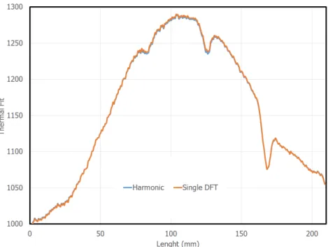
3.29 Difference between the amplitude averaged profiles, using Harmonic and single DFT . . . 73
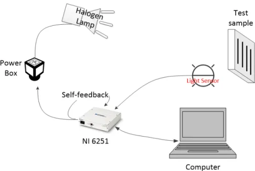
4.1 Light sensor box and physical connections . . . 78
4.2 Schematic of the stimulation characterization with the light sensor test. . . 79
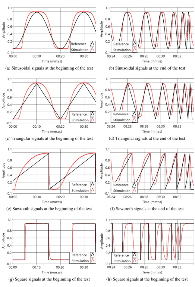
4.3 Reference signals and correspondent stimulations at the beginning and end of the characterization tests . . . 81
4.4 Reference signals and correspondent stimulations at the beginning and end of the characterization tests . . . 83
4.5 Stimulation dynamic response (Bode plot) . . . 85
4.6 Example of temperature curves during the thermal tests with optical feedback with 15 cycles . . . 87
4.7 Thermal fitting results for the lock-in tests using the optical feedback . . . 88
4.8 Amplitude average profiles obtained with the optical feedback . . . 90
4.9 Averaged cross-section profiles for common and feedback LTT . . . 91
4.10 Setup of the thermal tests using the PID controller . . . 92
4.11 Example of temperature curves during the thermal tests with PID controller . . . 93
4.12 Temperature of sound area and at slot 4 for a feedback and PID LTT, during the 10 and 30 second cycle period . . . 95
4.13 Peaks and valleys observed during the tests . . . 96
4.14 Common LTT, feedback LTT and LTT with PID normalized profiles (cycle period of 20 seconds) . . . 97
4.15 Common, feedback and LTT with PID, normalized profiles with high-pass filter . 98 4.16 Comparison of the phase average profiles . . . 99
5.2 Example of mesh used in the numeric simulation with slots of 10 millimetres . . 107
5.3 Temperature profiles in the sample, for different number of elements in the Y direction . . . 108
5.4 Base area temperature profiles, for different number of elements in the Y direction 109 5.5 Temperature profiles for different number of elements in the centre of slot 4 . . . 109
5.6 Temperature profiles for different mesh in the area between slots . . . 110
5.7 Temperature profiles for different meshes in the mean area of slot 4 . . . 111
5.8 Temperature obtained in laboratory and by simulation, for a stimulation of 20 seconds in the central point of slot 4 . . . 112
5.9 Temperature profiles at frame 350 for the stimulation of 20 seconds . . . 113
5.10 Temperature evolution at the centre of slot 4 for different stimulus duration . . . 115
5.11 Temperature at the end of the stimulation in the centre of the four slots . . . 116
5.12 Temperature profiles in the stimulation boundary . . . 117
5.13 Temperature evolution where the stimulus is being applied . . . 120
5.14 Temperature difference between slots and its surrounding areas function of stimulus period and instance being analysed . . . 121
5.15 Temperature difference function of the PMMA sample thickness and stimulation period, red and green dots represent the maximum and recommended stimulation period . . . 123
5.16 Temperature difference function of the CFRP sample thickness and stimulation period . . . 125
5.17 Temperature obtained in laboratory and simulation in the centre of slot 4 . . . 126
5.18 Temperature profiles at the end of the test in the stimulation surface (20 seconds) 127 5.19 Temperature evolution at the centre of slot 4 . . . 129
5.20 Temperature profiles in the stimulation surface after 15 cycles . . . 131
5.21 Amplitude responses from the stimulation surface after 15 cycles . . . 133
5.22 Phase delay of the stimulation surface after 15 cycles . . . 135
LIST OF FIGURES xv
5.26 Phase difference function of cycle period, number of cycles ans for slots 1 to 4 . . 142
5.27 Amplitude difference function of PMMA sample thickness and cycle period . . . 144
5.28 Phase difference function of the sample thickness and cycle period of PMMA samples . . . 145
5.29 Amplitude difference function of the samples thickness and cycle period, for CFRP 146 5.30 Phase difference function of the sample thickness and cycle period of CFRP samples.147 6.1 Average temperature cross section profiles (10 millimetre width) . . . 151
6.2 CFRP sample geometry . . . 152
6.3 Vertical temperature profiles for the CFRP sample . . . 153
6.4 Average cross section profiles from several LTT . . . 154
6.7 Radiation in the thermal image acquisition and their relationship . . . 158
6.9 Images obtained by different techniques . . . 162
A.1 Test sample and set-up . . . 174
A.2 Crack evolution in initial tests . . . 175
A.3 Thermal results for the flat bar tests . . . 177
A.4 Crack thermal patterns . . . 178
A.5 Thermal profiles along the crack tip . . . 179
List of Tables
2.1 Fibres main properties . . . 13
2.2 Resins main properties . . . 14
2.3 Main dye penetrant characteristics . . . 18
2.4 Radiographic testing main characteristics . . . 21
2.5 Main characteristics of the refereed NDT techniques . . . 27
3.1 Temperature sensors . . . 30
3.2 Infrared wave sub-bands . . . 33
3.3 Main characteristics of transient light stimulation . . . 41
3.4 Main characteristics of light modulated stimulations . . . 42
3.5 Main characteristics of microwaves used as stimulation . . . 44
3.6 Characteristics ultrasounds used as stimulation . . . 45
3.7 Characteristics mechanical loads used as stimulation . . . 46
3.8 Resume of all the parameters that can be combined among themselves . . . 51
3.9 Values of the c parameter in the used samples . . . 52
3.10 Thermal difference limits for all plates . . . 55
3.11 Resume of all the parameters that can be combined among themselves . . . 63
4.1 Values of the several normalized LTT, for slot 4 . . . 98
6.1 Recommendations for Infrared thermal tests . . . 160
Symbols
α Angle between the stimulus radiation and the temperature radiation (rad) β Volumetric thermal expansion coefficient ()K1)
∆ Gradient of a certain variable (in all direction)
δ Gradient of a certain variable (in a specific directions) ε Emissivity (-)
λ Wavelength (m)
µ Dynamic viscosity (s×mkg )
∇ Backward difference operator in a differential operation
φ Generic variable used in differential equation and in this work representative of a generic temperature (K)
ρ Relative density
σ Stefan Boltzmannconstant, 5.67×10⁻⁸ (m2W×K4)
θ Angle between the stimulus radiation and the measured radiation (rad) υ kinematic viscosity (ms2) ς Heat capacity (KJ) A Area (m2) AS Amplitude surface (K) B Boltzmann constant (1.38 × 10⁻²³ J K)
c Ratio between the sample remaining thickness and the defect width (-) c0 Speed of light (ms)
Cp Specific heat (kg×KJ )
CP Stimulation cycle period p (s) g Gravitational acceleration (m s2) Gr Grashoff number (Ra Pr) K Thermal conductivity ( W m×K) l Sample thickness (mm) xix
Lc Characteristic length (m)
m Mass (kg)
MR Measured radiation ( W m2×Sr×nm)
Nu Nusselt number (-)
P Energy radiated by a blackbody according to the Plank law ( W m2×Sr×nm)
Pr Prandtl number (-) PS Phase Surface (rad)
Q Total of energy transferred by heat (J) Qi Interior heat source per unitary volume (W) q Heat flux (W/m2)
Ra Rayleigh number (-) Re Reynolds number (-)
S Energy radiated by a blackbody according to the Stefan–Boltzmann Law (J W)
SP Stimulation Period, r on appendix (s) Sr Steradians, solid or tridimensional angle (sr) t Time (s)
T Temperature (K)
T0 Temperature at initial time (K)
T∞ Temperature at infinite, also called ambient temperature (used 297.15 K)
Ts Temperature at given surface (K)
TS Transient surface (K)
TR Temperature radiation ( W m2×Sr×nm)
Tr Transmittance, capacity of a body to transmit radiation (-) SR Stimulus radiation ( W
m2×Sr×nm)
u Generic direction (X, Y or Z) V Volume (m3)
Glossary and Abbreviations
AE Acoustic Emissions, sound emission from anomalies existing in a component
AT Active Thermography
ApT Apparent Temperature, the temperature of an object as determined solely from the measured radiance, assuming an emissivity of 1
ASTM American Society for Testing and Materials ATT Active Thermal Testing
CFRP Carbon Fiber Reinforced Polymers CMC Ceramic Matrix Composites
CT Computed Tomography, tree dimensional image technique possible through the combination of several X-ray images
DFT Discrete Fourier Transform DIC Digital Image Correlation DIRT Digital Infrared Thermography
ESPI Electronic Speckle Pattern Interferometry FAA Federal Aviation Administration
FDM Finite Differences Method FEA Finite Element Analyzes FEM Finite Element Method FIR Far Infrared
FVM Finite Volume Method IR Infrared
IRNDT Infrared Nondestructive Testing, is also the name of the commercial program used in this work
IRT Infrared Thermography, indirect temperature measurement (as an image) by measuring infrared radiation
IRTT Infrared Thermal Testing xxi
LDR Light Dependent Resistors LED Light Emitting Diode LTT Lock-in Thermal Testing LWIR Long Wave Infrared
MCT Mercury Cadmium Telluride MMC Metal Matrix Composites MWIR Middle Wave Infrared
NDE Non Destructive Evaluation, evaluating a component to access its integrity or determine the extension of a damage without destroying it or further compromise it
NDT Non Destructive Testing, testing a component to access its integrity without destroying it or compromise it
NI National Instruments NIR Near Infrared
NETD Noise Equivalent Temperature Difference, target-to-background temperature difference between a blackbody target and its blackbody background at which signal-to-noise ratio of a thermal imaging system or scanner is unity
PAN Polyacrylonitrile, method to develop carbon fibers PAEK Polyarylketone
PDE Partial Differential Equations PE Polyethylene
PEEK Polyetheretherketone
PID Proportional Integral–Derivativecontrol loop feedback mechanism acting in the feedback signal, its integral and derivative signal
PMC Polymeric Matrix Composites PMMA Poly-methyl-meth-acrylate PP Polypropylene
PPS Polyphenylene Sulfide
RT Radiographic Testing Nondestructive testing method using Gamma or Neutron emissions to scan a component
SIF Stress Intensity Factor
SL Stimulus Length, duration of the stimulation in a transient analyses or cycle period in a lock-in test
SR Stimulus Radiation, infrared radiation measured by the infrared thermal camera resulting from an optical stimulation source
SYMBOLS AND ABBREVIATIONS xxiii
ST Sample Thickness, nominal thickness of a sample SD Standard Deviation
SWIR Short Wave Infrared
TF Thermal Fit, curve fitting to temperature data from active infrared thermal tests
Tr Transmittance
TSA Thermal Stress Analyses, or Thermoelastic, is the determination of the mechanical stress by application of a fast oscillation load and measure its local temperature variation.
TSR Thermal Signal Reconstructionprocessing algorithm used to obtain better results in infrared thermal tests
TTT Transient Thermal Testing
US Ultrasound, sound waves with frequencies higher than the audible by humans (typically 20 kHz)
Chapter 1
Introduction
1.1
Context
The search for lighter, stronger, and more reliable materials is a daily concern in the majority of the industries. In particular the transport industries can benefit with the discovery of new and better performing materials. This constant evolution led to the creation of composite materials. From the vast number and type of composite materials available today, Carbon Fiber Reinforced Polymers (CFRP) have distinguished themselves as one of the better performing materials. They have very good mechanical properties without having a high manufacturing and processing cost [1]. However, in the transport industries there is a huge concern with security and maintenance operations. An adequate maintenance is essential to guarantee the vehicle safety, and its users, along with a good comfort. This aspect is far more critical in aeronautics, where a failure can result in a catastrophic event.
Non-destructive tests (NDT) are the natural solution when choosing methods to detect and characterize defects during maintenance operations. Over several decades the available techniques have evolved, like mentioned by Jayamangal Prasad and others [2]. Some of these have evolved from single point techniques and those same principles are now used in image techniques. Giving the possibility to scan a component or structure, faster and with the same accuracy. They are usually easier to interpret and the defects are easily identified. Image techniques usually measure a portion of the electromagnetic spectrum to create an image. In particular Infrared Thermography (IRT) has managed to detect anomalies where many others fail, have difficulties or are time consuming. IRT measures the infrared radiation, normally the middle and far sub-bands, that is related with the object temperature.
There are several NDT techniques that use thermography, however active thermography tests (ATT), where a stimulation is applied to the object, are the most effective. During the application of the stimulation to the object or/and some time after its ending, the temperature is monitored and recorded. The processing phase is one of the most critical parts of the thermal analyses. There are
two main types of tests that use thermography as a measurement tool: single stimulation (Transient and Pulse) and cyclic stimulation tests (Lock-in and TSA). Despite being different techniques, Transient and Lock-in thermal testing, they use very often the same type of stimulation source to detect the same type of defect. Although they present some similarities, the methodologies and processing procedure are considerably different. These techniques, require the specification of some parameters: waveform, stimulation or cycle period, instant to analysis, number of cycles, temperature interpolation model used by the software manufacturer, etc.
Being able to extract more information from a thermal test adds more value to a technique that already is extremely used. The improvements in post-processing have the advantage of maintaining the current physical measuring systems, thus preventing added costs to any alteration. Therefore, this work aimed to improve the accuracy in the selection of the parameters used to perform a thermal analyses and provide a guide to the expected results.
1.2
Main Goal
The main goal of this work is to develop a prediction model that provides the ideal parameters and settings to conduct active infrared thermal tests in composite materials with higher sensitivity to defects defection. The development was oriented to detect defects in composite materials, with special emphasis on carbon fiber reinforced polymers. To accomplish this objective, several tasks were defined:
• State of the art review relating non-destructive tests, with special emphasis in thermography techniques;
• Non-destructive thermal tests using thermography, with specimens build specifically to identify and characterize the settings that produce the best results;
• Simulation of thermal tests to increase the comprehension of the heat flow and behaviour during a thermal NDT test;
• Development and validation of a prediction model to perform thermal testing with a higher accuracy and its validation with reference components.
1.3
Structure
This work is divided in seven chapters. The current and first chapter is the introduction to the document. Here are described the main goal and the context of this work.
The second chapter relates the state of the art. This covers two main topics, composite materials and non-destructive testing. The composite materials description is oriented to polymeric
1.3 Structure 3
matrix and fiber reinforcements. The sub-chapter referring to non-destructive testing, briefly mentions the most relevant aspects of each NDT technique. A short description of the stimulations sources used in thermal testing is also mentioned.
The third chapter starts by introducing temperature measuring techniques with a main focus in infrared thermography and the several parameters used in the process. Next are presented and discussed the results obtained in laboratory with two main techniques: transient and lock-in tests. In both cases, are compared and discussed the influence of the most important parameters in the tests and in the post-processing. At the end are identified the settings that produced the best results. The fourth chapter introduces thermal testing using stimulation feedback and with an active controller. The first part uses a light resistive sensor in the system to obtain the optical feedback. The second part, uses that same feedback along with a PID controller to achieve an accurate optical stimulation waveform. At the end of the chapter the three alternatives are compared: the common thermal tests, with feedback and with the controller.
Using the information collected in laboratory tests, finite element simulations were performed to achieve a better understanding of the heat flow during the most relevant tests. In this fifth chapter are presented and described the assumptions, the mathematical models, results and analyses of the simulations. With the results from the simulations, were found several equations that modulate the ideal stimulation parameters and expected results.
The sixth chapter validates the previously described models. Here, the models for the transient and lock-in thermal tests are validated from samples with different geometries and build with different materials, such as CFRP. At the end of this chapter the two techniques analysed in this work and phase shearography are compared.
The final and last chapter has the work conclusion. Here are briefly mentioned the most important comments and results contributions. Some brief notes and recommendations about future steps are also mentioned.
At the end of this document three appendixes are presented. The first is a brief analyses of the Thermoelastic Stress Analyses (TSA), with a special focus in the influence of the load in the thermal and resulting mechanical stress. The second is a resume of the prediction thermal response from the simulations. The third presents technical drawings of the main samples used and analysed in this work.
Chapter 2
State of the Art
This chapter is divided in two main sections, relating composite materials and Non-Destructive Testing (NDT). Both present a global overview of the corresponding field, justifying the importance of carbon fibre reinforced polymers and active infrared thermal testing.
Composite materials can be divided into classes, depending of their composition, structure and manufacturing techniques that will be shortly introduced giving an overall overview to the world of composite materials. The polymeric matrix composites and their reinforcements using fibres are described in a greater detail, since it is a relevant matter to this work.
Currently, several NDT techniques can be used to detect and characterize defects in composite materials. Starting with the most simple one, visual inspection also describing ultrasounds and radiographic, among others, several NDT techniques are mentioned and described. Despite not being the main goal of this work, this provides a better understanding of the alternative techniques to infrared thermography used to perform NDT. Here are reviewed the main and more common NDT technologies, their core principles and characteristics.
2.1
Composite materials
Composite materials are an association of two or more different materials, resulting in combined material with characteristics differing from any of the initial ones. The most common arrangement is the dispersion of the reinforcement in a continuous base (matrix). The reinforcement is usually much stronger than the matrix, but the high properties of a composite, appear when they are combined in an appropriate relative contents, orientations and dispersions [3]. According to their macroscopic structure and reinforcement disposition, composite materials can be divided into four categories [4]:
• Fibrous Composites— Composed by a matrix and fibres. These fibres are long and thin (typically 20 µm in diameter), these composites frequently have extremely high mechanical properties in the fibre main direction;
• Laminated Composites— Composed by layers of several materials bounded together to form a high performance compound, typically in the form of a plate or shell;
• Particle Composites— Composed by small particles dispersed in a matrix. These particles usually have one long dimension and tend to produce a highly isotropic composites; • Mixed— A combination of any of the previously mentioned.
The most common composite materials uses fibres as its main reinforcement. Usually it increases the mechanical properties of the matrix, making the composite very strong in the fibres main direction [5]. In most of the situations the matrix is a resin. Since the composites present very high properties in the direction of the fibres, these can be disperse in a certain configuration to optimize the performance of the composite [6]. The composites reinforced with fibres can be divided in three categories, dependent of the material used in its matrix:
• Ceramic Matrix Composites (CMC) — The matrix is composed by a ceramic and the reinforcements are usually fibres (short fibres). They are commonly used in environments with high temperatures;
• Metal Matrix Composites (MMC)— These materials use metals for the matrix (aluminum among others) and are reinforced with fibres, the automotive industry is an area where they are more commonly used;
• Polymeric Matrix Composites (PMC)— Polymeric based resins are generally used in its matrix and fibres for the reinforcement, they are also referred as fibre reinforced polymers (FRP).
2.1 Composite materials 7
2.1.1 Ceramic matrix composites
Ceramic composites were initially manufactured using ceramic materials in the matrix and in the reinforcements. However, nowadays is also common to use fibres as reinforcement. The highest advantage of ceramic composites is its resistance to high temperatures, therefore they are naturally selected to be used in these environments and conditions, some of these were described by Aldo R. Boccaccini in [7]. The ceramic matrix usually provides high: strength, elastic modulus, hardness and temperature resistance and dimensional stability. The most common type of ceramic composite is by far the glass fibre. The majority of fibres used present an individual diameter of approximately 10 µm. With this small diameters they are capable of flexing, keeping their original stiffness and brittleness, natural of the glass [7]. Being one of the first fibres to be processed industrially, they are still used in a variety of products and components and in some cases, with techniques with several decades [8].
The fibres used in this types of composites can also be cropped in short segments and have them mixed and randomly dispersed in the matrix [9]. If the fibres are short enough, they can be mixed, injected into a mold or even projected onto a surface. This surface could be a mold (a more common situation) or a structural component that is being reinforced, this is explained in more detail by Krishan K. Chawla in [10]. With these materials and manufacturing processes, is possible to produce components with a complex shapes and highly optimized. Here they can have different thicknesses and the mechanical properties can vary in some sections of the component. This type of processing is typically used in large parts like car components and bodies, boats, pressure vessels and pipelines. Most common matrices are chemical inert, these materials are also indicated for corrosive or other damaging environments.
2.1.2 Metal matrix composites
Like suggested by its name, Metal Matrix Composites (MMC) use metals in their matrix, in particular aluminium is widely used in the matrix of MMC. This mainly because of the processing methods developed in the 1970s (foil-fibre-foil method), taking advantage of the low processing temperatures of the aluminium compared to other metals [11]. The result is aluminium composite reinforced with continuous boron fibres and another reinforced with SiC-coated boron fibres. Currently, the MMC based on aluminium can be provided for a direct product application (raw alloys) or to undergo future processes. MMC can posteriorly pass through heat treatments to further improve their properties. Some examples of the research in this area was pioneered by Suganuma and Kainer [12,13].
Titanium alloys usually present a density of 4300 kg/m3, being 40% lighter, but with the same
strength of the majority of steels. For temperatures up to 300◦C, titanium maintain good structural
capable metals, its usage in a composite matrix results in one of the most capable materials, usually used in extremely demanding conditions such as the aerospace and aeronautical industries [15].
The reinforcements in MMC may take a discreet arrangement and disposition, leading to a network of individual fibres. As a result, strength and rigidity are improved. Usual reinforcements are nitrides, carbides and oxides, precisely characterized by their strength and rigidity despite the temperature. A short introduction to this matter is performed by Karl Kainer in its book, Metal Matrix Composites [16]. The reinforcements can be short particles or whiskers or long fibres. Despite the short reinforcements, the load is still mainly supported by the fibres while the matrix acts as a restrain for the reinforcements. With the long and continuous or semi-continuous fibres, the supported main load can have higher magnitude, with the matrix still being used to hold the fibres in place and distribute the load.
Some fibres can be coated with an additional reinforcement before the junction with the matrix. The coating usually improves the bounding with the matrix, to achieve cohesive structure, like explained by Kainer [17]. This has a protective role and prevent the fibre diffusion within the matrix, by preventing a direct contact between the two. Alongside these advantages, it is also achieved this way a better distribution of internal thermal and mechanical stresses. The coating also has a protective role during the manipulation and manufacturing processes. There are several manufacturing processes, being the most important:
• Powder blending and consolidation; • Consolidation diffusion bonding; • Vapor deposition;
• Squeeze casting and squeeze infiltration; • Spray deposition;
• Slurry casting; • Reactive processing.
2.1.3 Polymeric matrix composites - resins
Polymeric matrix composites (PMC) are the most common and used composites in aeronautics industry [18]. Resins are a common material to be used as matrix and will be described here, followed by the fibres. The word resin, as described by Anthony Kally, is referred to a polymer that can be described as mixture of various additives or chemical reactive components [19]. Usually the resin determine the final shape of the composite, therefore, its properties define the handling and processing procedure. The main type of resins are:
2.1 Composite materials 9
• Epoxy; • Polyester; • Phenolic;
• Thermoplastic materials (Polyimides and silicones); • Bismaleimide.
An epoxy resin is a polymer characterized by an oxirane structure, a three-member ring with one oxygen and two carbon atoms [20]. They are curable be reacting with acids, amides, amines, alcohols, phenols making them a thermosetting resins [21]. After the curing process they present elevated elastic modulus and strength, excellent adhesion, good chemical resistance, low shrinkage (when compared before the cure process) and are fairly ease to process. The biggest disadvantage is the high brittleness and its sensibility to moisture. The cure process takes place between room temperature and 180◦C, being the most common in the range of 120 and 180◦C.
The cure temperature also influences the resin behaviour and properties after the cure. The curing pressures are low, ranging from vacuum to 700 kPa.
The polyester resins (thermosetting) are economical and fast to process, therefore, they are used for low-cost applications and products. These resins are a combination of polyesters in a monomer solution, generally styrene [22]. This improves the handling of the resin and enables its molding without pressure. Several ancillary products are used to mold the resins, such as:
• Catalyst– Start the chemical reaction (cure process), adds an extra substance to the final composition and reduces the energy involved in the process;
• Accelerator– Increase the rate of the chemical reaction (cure process) and can be consumed during the process;
• Addictives:
– Thixotropic– Improve the resin viscosity behaviour prior to the cure for molding and injection applications;
– Pigment– Add colour to the mixture, mainly for cosmetic purposes;
– Filler– Reduce weight, change specific molding characteristics and reduce costs; – Chemical and/or fire resistance – Add or increase its impermeability to a certain
chemical or increase the fire resistance capabilities.
Phenolic resins, are characterize by having a matrix that is thermal resistance to chemical and smoke. The most common types are resole and novolac, according with their condensation reaction. From their high viscosity and molecular weight, comes their natural capability for unusual conformations or complex shapes. These applications are also enhanced by the capability of curing supporting high temperatures and free-standing post-curing processes. The normal cure of these resins can be performed under pressure or autoclave [23].
Polyamides resins are a family of diverse polymers that contain aromatic circular heterocyclic structure. They can be thermoset or thermoplastic resins, in particular thermoplastic polyimides can be thermoset if a post-cure high temperature is applied, the opposite situation is also possible. Polyimide resins require a cure temperature near 90◦C, and have an operation temperatures range
from -150 up to 200 ◦C. Even at high temperatures they are capable of keep good mechanical
properties and are dimensionally stable. Being one of the resins with better properties, their primary use is in circuit boards, hot engine parts and aerospace structures [24].
Another type of resins are thermoplastics. These, can be semi-crystalline or amorphous, with these last corresponding to the majority. Some semi-crystalline thermoplastics are: polyethylene (PE), polypropylene (PP), polyphenylene sulfide (PPS), polyetheretherketone (PEEK) and even polyarylketone (PAEK) [25]. These tend to be very malleable and can be processed into powders, filaments and films. Their usage in primary and secondary structures of aerospace industries is due to the resistance to flames, mechanical properties at high temperatures, after an impact and moisture absorption. Some of the most important amorphous polymers are: polysulfone, polyamide-imide, polyphenylsulfone, polyetherimide, polyether sulfone, polyarylate, polystyrene and polyphenylene sulfide sulfone [26]. These resins are easy and fast to process, their mechanical properties are good, particularly their resistance at impacts and present an excellent hardness [27]. Another type of thermosetting resins are Bismaleimides, resulting from the reaction of a diamine and maleic anhydride. They are generally available as "prepreg" forms, rovings, and sheets of fabrics, among others. Another important characteristic is the extreme adaptability to the reinforcement properties, being dependent of the used reinforcements [28]. The capabilities of bismaleimides are comparable to epoxy with the biggest differences being the glass transition temperature (around 260 to 320◦C) and two to three percent higher elongation. This without losing
excellent performance at ambient and high temperatures. The processing and resulting products are very similar to epoxy resins [29].
Silicone resins have a three-dimensional structures primarily composed by organosilicon. They can endure temperatures of 350 ◦C, and with the appropriate fillers, 600 ◦C could be tolerated.
They are one of the resins with higher oxidation resistant, hydrophobic and vapour permeability. The global mechanical properties are also very good, including weathering resistance and their dielectric behaviour is also very good [30].
2.1.4 Polymeric matrix composites - fibres
The most used composite materials are reinforced with fibres and can be very isotropic or highly anisotropic. The fibres are a very important part of the composite and usually are the responsible for the improvement of the matrix properties. The most used types of fibres are:
2.1 Composite materials 11
• Carbon and graphite; • Aramid; • Glass; • Boron; • Alumina; • Silicon carbide; • Quartz.
Carbon and graphite are the most known reinforcement fibres, with great flexibility and a variety of properties that can be adjusted. A polymer reinforced with these fibre will result in a component that is stiff without being brittle. They were used commercially for the first time when Thomas Edison created the incandescent light bulb [31]. The carbon fibres as they are known today were firstly discovered by Roger Bacon, this is also considered the first reference to nanotubes [32]. The carbon fibres are composed of small filaments with 5 to 10 µm in diameter. The fibres can be arranged in three main dispositions depending on their origin: rayon, polyacrylonitrile (PAN) or pitch. The rayon fibres were the first ones to be commercialized (1960), however they have been gradually replaced by the superior PAN type since the 70’s [33]. The pitch fibres are able to achieve ultra-high Young modulus and thermal conductivity, being the current choice for critical space and military applications and also very expensive.
Aramid fibres are synthetic fibres that are heat resistant with rigid polymer chains. They are more commonly known as kevlar R or Nomex R. Their most important characteristics are:
high strength, resistance to abrasion and organic solvents, non-conductive no melting point, low flammability and good fabric integrity at elevated temperatures [34]. On the downside, they are sensitive to ultraviolet light, being gradated when exposed to sun light. The main and first major application of these fibres is in protective gears like bullet proof vests. Being flame resistant, self-extinguishing and low conductivity, they are a natural choice for wire casing and fire fighting protection equipment [35].
Like many others, glass fibres reinforcements consists in several extremely thin fibres, in this case made out of glass [36]. The most common is the E-glass fibre, they are composed by alumino-borosilicate. The mechanical properties of these fibres are fairly similar to others, even if a little inferior than carbon fibres. Despite a little more ductile and less strong when compared with some types of carbon fibres, their cost is considerable lower, with its brittleness diminished and controlled when used in composites. The fibres can assume an amorphous configuration and be used in building heat insulator or arranged in a textile and introduced in a polymeric matrix. This last application gives origin to strong and relatively lightweight fibre-reinforced polymer with low production costs.
The Boron fibres present an amorphous arrangement of their elements. They are usually manufactured by a deposition reaction on hot tungsten wire which leaves tungsten boride in the core of the fibre. These fibres present a high strength and elastic modulus with small density. They are exclusively available in the filament form or prepreg by epoxy matrix. The boron fibres are considerably expensive (more than carbon fibres), being used in some components in the aerospace and aeronautics industry like F-14/15 stabilizers reconnaissance satellites, and several parts of the space shuttles [37].
Alumina fibres in a polycrystalline form, are ideal to reinforce plastics, ceramics and metals. They can be provided for reinforcements as long or short fibres having good mechanical and chemical resistance. They are good thermal and electrical insulators and their manufacturing cost is comparable to the carbon fibres. Long fibres are ease to align and handling. Over the last years, alumina/epoxy and aramid/epoxy hybrid composites reinforced with alumina and aramid fibres have proved valuable materials in radar transparent structures and high performance electronic circuit boards [38].
Silicon carbide fibres normally possess diameters of 140 µm and present high strength elastic modulus and density. They are oriented to be used as reinforcements of aluminium and titanium alloys, either lengthwise or crosswise. The cure cycles resemble the ones applied in carbon and glass fibres. Being used as reinforcements, their solo properties are not relevant and the composite is highly dependent of the matrix properties [39].
Quartz fibres are used almost in its pure state, with percentages above the 99.9 % fused with silica glass fibres. In the majority of the situations, the fibres are coated with an organic binder, the silane coupling agents endow the fibres with a high compatibility with many resins. Quartz fibres present the highest strength-to-weight ratio, being even higher than the high temperature materials (commercially available). They do not melt or evaporate for temperatures up to 1650
◦C and are used in situation were the service temperature is over 1000◦C. The chemical stability
and resilience are also very high, with the exception for highly alkaline environments. Despite the high cost these fibres are also used as electrical insulators [40].
2.1.5 Nanotubes and mechanical properties overview
In the past decade, nanotubes have been one of the most studied subjects. Their mechanical and electrical properties have been studied intensively with new applications being constantly discovered. The properties of the carbon nanotubes make them the most appropriate additional reinforcements for specific composite applications. Along with Roger Bacon in 1960 [32], Sumio Iijima in 1991 is considered the father modern carbon nanotubes [41]. Since then, several have reported their high mechanical and physical properties. Namely the modulus, reaching values near the elastic modulus of diamond and strength up to 100 times higher than the better steels,
2.1 Composite materials 13
maintaining a low density. Another important characteristic is their very high thermal conductivity. These properties make them one of the most promising reinforcements to be used in nanocomposite materials. The thermal stability, for temperatures up to 2800◦C, is also very high, along with a
capacity to carry electric currents, 1000 times higher than copper [42], [43]. Reinforced with nanotubes, MMC present superior elastic modulus, ultimate tensile strength and yield strength [44]. These composites can have their properties even higher depending on the type of process used (solid or liquid-phase) [45], [46].
Currently are known two types of nanotubes. The first consists in a single sheet of carbon, rolled to a cylindric with a diameter of approximately 1 nm and reaching up to a few centimetres [47]. Nanotubes with multiple walls are formed with several concentric cylinders of carbon sheets. The separation between cylinders is approximately 0.35 nm, which is similar to the distance of planes in graphite [41]. The nanotubes can have diameters ranging from 2 to 100 nm and lengths of some tens of microns. In the present days some researchers have clammed distances of approximately 0.5 meters [48]. In current days, the most common manner of obtaining the nanotubes is by chemical vapour deposition and laser ablation [49], [50]. One of the biggest challenges in the production of composite materials is to achieve an uniform distribution of the nanotubes and consequentially the loads applied to the composite. The load distribution is obtained when exists a dispersion of the carbon nanotubes in the matrix, an optimum blending and the correct alignment of the nanotubes in the matrix.
The unknown behaviour of the newly discovered composite materials makes difficult their usage in production lines or high production rates. Despite the recent discoveries in composite materials, carbon and glass fibres are still the most common. Table2.1 presents an overview of the main properties of common fibres used in composite materials.
Table 2.1: Fibres main properties Tensile modulus (GPa) Tensile strength (MPa) Density (kg/m3) Fibre diameter (µm) Carbon [51] 41 - 760 150 - 1000 1600 - 2150 4 - 11 Aramid 135 410 1400 5 - 60 Glass 70 - 12.5 440 - 670 2480 - 2620 30 Boron 400 730 - 1000 2300 - 2600 100 - 200 Alumina 385 1.4 3900 20 Silicon carbide [52] 48 - 66 17 - 170 2.5 - 3.2 7 - 140 Quartz 72 6 2.2 0.9 - 1.1
Very often the matrix main function is to support and maintain the fibres in their respective place, leading to two facts. Firstly, the most part of the structure weight is due to the matrix. Second, the matrix plays the main role in the manufacture procedures. Looking at table2.1, it is easily observed that carbon fibres present one of the highest tensile strength alongside with Boron fibres. On the the downside, Boron fibres present higher density than carbon fibres. In table 2.2
are exposed the main resins used with carbon fibres. Epoxy resins are low cost and are easy to produce, this made them one of the most used, despite not possessing any particular property that differentiate them from others resins.
Table 2.2: Resins main properties Tensile modulus (GPa) Tensile strength (MPa) Compressive strength (MPa) Density (kg/m3) Epoxy 10.5 85 190 1100 Polyester [53] 3.4 55 -80 120 1900 - 2000 Phenolic 10 50 — 1400 Polyimides 4.5 152 220 1400 Silicon[54] 2.1 15 — 1000
2.2
Non-destructive testing
Although the surface defects on structures are easier to detect by the naked eye, the inner defects require the use of auxiliary inspection techniques, such as Non-Destructive Testing (NDT) [55,
56]. This way, it is possible to detect and quantify the damage in a structure, or component, without diminish their life span. In this case, the areas to be analysed are stimulated to reveal the presence of discontinuities or changes in structure, usually coincident with defects. The behaviour of the structure in regions of interest are monitored and may also be compared with previous tests or new components.
There are currently various non-destructive inspection methods (NDT) [57]. However, none of the known techniques can fully meet all the needs of NDT in composites. The ultrasound techniques developed over the past decades are one of the most common and reliable techniques. However, the time required to perform the evaluation of an area using ultrasounds is considerably high and require inspections coupling means, water or gel, this fact prevents the inspection of hydrophilic materials. The most commonly used non-destructive tests are:
2.2 Non-destructive testing 15 • Visual inspections; • Penetrant inspection; • Electromagnetic testing; • Radiographic testing; • Acoustic emission; • Laser testing; • Vibration Analysis; • Ultrasonic Testing; • Infrared thermography.
For the correct selection of a NDT technique, some considerations are required. The object manufacturing processes and usage conditions, along with the expected defects are some of the most important aspects. Depending on the nature of the expected defects, they can be visible or hidden. To detect a defect, a pass/reject criteria should be defined. Should also be taken in consideration the spatial resolution of the selected technique, along with maximum defect size, supported by the component without compromising its integrity.
2.2.1 Visual inspections
During the first years of aviation, visual inspections were considered to be very subjective and difficult to be re-evaluate or compared since it was not possible to record the data. The operator experience, conditions of the test, cleanness, quality of the optical equipment used and illumination are important aspects of these tests [58]. The evolution of technology leads to the acceptance of visual inspections as a NDT by the American Society for Testing and Materials (ASTM) and Federal Aviation Administration (FAA) to the creation of standards to conduct these tests [59]. Some considerations about this matter is presented in one of the firsts great references in visual inspections by Robert Anderson [60].
Visual inspections can use auxiliary equipment (micrometres and spring loaded depth gauges, among others). For example, when evaluating the corrosion depth on a pipe, appearance and colour of a surface can provide useful indication on the origin and damage extension. Visual inspections are usually used to conduct minimal and fast evaluations, but by using optical equipment it is possible to access defects with a greater detail. The most used equipment’s are:
• Borescopes;
• Fibrescopes and Videoscopes; • Microscopes;
• The Long-Distance Microscope;
Borescopes are optical devices, consist in a long tube, flexible or rigid, with a lenses at one end and a display device at the other. Near the lenses are located an optical fibre and light to illuminate the observation area. Due to its geometry, borescopes are usually used to inspect pipes, tubes, dangerous access zones or other areas difficult to reach like the internal parts of jet engines. Nowadays they are being more and more used in the most divers situations, motivating the development of borescopes that are rigid, extensible, flexible, with micro designs and small amplification capabilities. The diameter, length, rigidity, illumination and amplification are the most important characteristics of these devices and define if a certain model is appropriated for a specific application or to locate a certain type of defect.
The modern fibresopes and videoscopes have overcome many of traditional limitations of the conventional processing and recordings by saving the images in real time. They have become more flexible, thin and reliable. The introduction of optical fibres and electronics, pushed the application range mainly by introducing LED light. The usage of laser lights can provide measuring capacities to visual inspections. Some of the multiple accessories available are: optical adapters (mono and stereo), side viewing optics, wide and extra narrow lenses and remotely controlled flexible cables. The introduction of the microscope, gave a new insight in non-destructive evaluation. They use visible light and lenses to amplify a certain detail. The observation can be captured by a camera and recorded to future analyses. The main usage is the observation of very small components like jewels polishing, electronic circuits or in the analyses of micro-structure made out of alloys or composite materials.
An alternative to the standard microscope is the long distance microscope and continuously focusable microscope. They are considerable smaller than the standard microscope, but cannot provide the same amplification level. The portability of these devices means they are appropriated to field measurements and applications. In some cases they can have accessories like, illuminations systems, lasers, cameras and others.
One form of increasing visual inspections are known as remote visual inspections. They use a digital video equipment to transmit the visual images to an off-site location, similar to what is described by Lorenz [61]. This type of inspections were initial used in applications were the area of inspection was inaccessible or dangerous. Nowadays, they are also used to centralize the decision making process and as a method to diminishing inspection costs. This type of inspection can use the above mentioned technologies either individually or combined.
Automated inspection uses certain specified parameters to determine the quality and integrity of a component or structure. This inspection method has gain popularity mainly by the evolution of machine vision technologies. Here a specialist defines the criteria of approve or rejection in a determined situation and the images are processed by a computer that access the integrity of
2.2 Non-destructive testing 17
the component. This technology can be easily combined with several others to enable guidance processes (robots and other automated systems), process control or even completely automated inspection.
2.2.2 Dye inspection
Dye or penetrant inspection bases its fundamentals in the usage of a substance that penetrates a crack or discontinuity by capillarity, from the surface to the crack interior. Despite the first mentioned date to 1920s in the steel industry, only in 1941 with the advances of Joseph Switzer, did this type of testing gain noticeable acceptance, witch lead to several patterns along the following years [62–65]. From then until today, the penetrant inspection have evolved continuously, from improved dyes, penetrant, emulsifier among others.
If looking solely at surface discontinuities, the current state of the art liquid penetrant are more accurate and reliable than radiographic tests. The best penetrant substances have a good penetrant capabilities while being able to remain in wide openings, without sacrificing its easiness of removing after the test is completed. A very important characteristic, especially in the case of composite material is the nonexistence of any chemical reaction with the component that can damage or diminish its integrity or even the composite appearance [66].
Due to its main principle, penetrant techniques are restricted to surface defect testing of witch they are very sensible and insensitive to the extension of subsurface defects [67]. On the opposite side, materials with elevated number of cavities and porous, like bronze porous alloys or unglazed ceramics will display an innumerable false defects. The most common of penetrant used are liquids with dye suspensions. Initially they are applied to the surface to be tested. After several minutes (depending on the used liquid type) during which the capillarity effect takes place, the liquid at the surface is removed. If a defect exists, a certain part of the liquid will be expelled and becomes visible, signalizing the presence of a surface discontinuity. In Table2.3are described the characteristics of the main types of penetrant liquids [66].
Water washable fluorescent liquids are produced with an oil base and with emulsifiers. Due to the oil base they can be easily removed with water. The designation fluorescent is derived from their ability to reflect a bright yellow light (usually) when illuminated with a black light. If a quantitative evaluation is desirable, it can be performed with a spectrometer sensible to ultraviolet light. Temperature changes the liquids viscosity, making them hard do appear in shallow defects (high temperatures) or harder to remove after inspection (low temperatures).
Post-Emulsification Fluorescent liquids are also produced with an oil base and a brilliant fluorescent additive. However these cannot be removed with plain water due to the missing emulsifiers. The emulsifiers are added after the liquid by pulverization or spaying, in a manner to
Table 2.3: Main dye penetrant characteristics Variable Water washable fluorescent Post emulsification fluorescent Water emulsification visible Solvent clean visible Sensitivity × × Visibility × × Fast test × × Retest × × Portability × × Shallow defects × Big components × × Black light × × Examiner influence × × Rough surfaces performance ×
obtain a uniform layer, allowing the removing of the excessive liquid. They are sensible than water washable fluorescent and are the easiest ones to reuse. Since they are easy to clean using water, they are recommended for components that have rough surfaces, like parts obtained by casting. Due to the high sensibility of these liquids, it is recommended the usage of black light not only to analyse the component but also for cleaning processes, prior to the examination.
Water emulsifiables penetrant liquids, require the application of a developer to the surface after the excess liquid is removed, usually with a white colour thus providing an even higher contrast to the test by contrasting with the coloured dye particles, increasing its sensibility. In some cases the marks are left visible after the test, to facilitate repair operations. Since they are oil-free liquids, anti-corrosion, coating, or welding operations can be performed after a simple clean process [68].
Solvent clean visible liquids are characterized mainly by being highly portable and therefore are largely used in field inspections since water or post-emulsification agent is not required. It is also a preferred liquid when, the usage of black light is a major difficulty. On the downside, it requires the existence of clean surfaces, free of oil, carbon, rust, grease, paint, or other coatings and impurities. These impurities may lead to false positives (false defects) indications. These types of liquids are applied direct from the containing aerosol recipient. The dwelling time depends of the required sensitivity, nature of the defect and surface conditions. The temperature is the major influence in the liquid viscosity and its capability to detect and highlight some defects [69].
2.2 Non-destructive testing 19
2.2.3 Electromagnetic testing
Non-destructive testing using electromagnetic principles can be divides into three main topics, Eddy currents, leakage flux and magneto-elastic tests.
Eddy current testing uses an alternating magnetic field, created by passing an alternated current through a coil. When the magnetic field approaches an electric conductive material it generates continuous Eddy currents. The induced Eddy currents penetrate in the material and are reflected to the coil. These reflected currents are inverse to the initially created ones and, will diminish the generated magnetic fields. When a defect exists in the component, this deviates the magnetic flux and consequentially the reflected eddy currents will change and diminish. Increasing the coil impedance, thus indicating a discontinuity or defect [70].
Since Eddy current testing uses the secondary, or reflected, magnetic flux to measure the material conductivity (smaller in the presence of a flaw), the material conductivity has a large influence in the technique sensitivity. Since the air has little magnetic conductivity, the distance and its variation to the surface is also extremely important. For very small distances and for small distance variations, the changes in the magnetic flux is linear. This distance variations can be measured in order to calculate the coil impedance for a zero distance between the coil and the object surface. The magnitude of the frequency influence is in the same order of the magnetic conductivity. Thus is possible to select a certain frequency that will result in a favourable operating point that maximizes the detection of defects with predefined characteristics.
The majority of tests that use Eddy currents do not require the precise measurement of the flux. In most situations the goal is to define a reference value for an area and then inspect the rest of the component surface, searching for flux variations that correspond to a defect.
If a testing prob with a single coil is used, the test will be greatly affected by the distance variation between the test piece and the prob surface. The probe will be affected by the component superficial rugosity and natural vibrations from the manipulation process. These difficulties can be overcome by using a coil with differential configuration. The movements affect both coils and therefore they compensate each-other minimizing these variations. In the presence of a defect, it will be sensed firstly by one then by the other coil. The comparison of the same defect measured by the two coils increases the system sensibility. The design of the coils shields may be used to shape the field and/or increase sensitivity and resolution [71].
Magnetic flux leakage testing uses the lines created in a component when a ferromagnetic material is magnetized. The existence of defect deviate and disrupts the flux lines enabling their detection by using leakage flux. With some limitations, is possible to characterize the extend of the defect by measuring the intensity of this flux [72]. These tests use magnetic sensors to detect