Genetic variability evaluation and selection in ancient grapevine varieties

Genetic Variability Evaluation and Selection

in Ancient Grapevine Varieties

Elsa Gonçalves and Antero Martins

Instituto Superior de Agronomia/Technical University of Lisbon

Portugal

1. Introduction

Contrary to what usually occurs with other crops, grapevine varieties are mostly landraces that were domesticated by humans centuries or millennia ago from populations of wild grapevines (Vitis vinifera ssp. sylvestris). It is logical to assume that domestication was not been a single, instantaneous act by any of the first farmers but was rather a long succession of negative mass selections of wild plants, followed by more stringent positive selections and a final selection of a single initial plant that was destined to become the source of a new variety.

Certainly, from early times, the first vines were multiplied through vegetative propagation because of two main reasons: (1) the high heterozygosity of the plants causes strong segregation during sexual reproduction, with a consequent loss of features that were previously selected for, and (2) the progeny plants take a long time to reach sexual maturity, resulting in a loss of productive capacity for several years. In contrast to sexual reproduction, vegetative propagation allows for the fast development of new, productive plants from an initial plant and ensures that previously selected traits are maintained. Selecting a single plant and vegetatively multiplying it creates a clone that consists of all of the genetically identical plants. However, although vegetative propagation ensures relatively homogeneous descendants, this homogeneity is not absolute. Indeed, the propagation depends on the growth of the tissues, on the cell division (mitosis) and on the DNA replication that occurs before each cell division. DNA replication is the source of gene mutations, that is, genetic variation. As a result, an initially homogeneous clone becomes genetically variable (a set of clones) over the course of time following successive multiplications. This set of genetically different clones corresponds to the variety that is presently cultivated.

Many of the genetic variations mentioned above are present in grapevines that are currently cultivated, and occasionally, we can directly observe the emergence of new features in vine plants. Typical examples are variations in the colour of the berry (for example, Pinot Blanc/Pinot Gris/Pinot Noir), the leaf's shape (for example, Chasselas/Chasselas Cioutat) and hairy leafs (for example, Garnacha/Garnacha Peluda). These types of features are determined by a single gene that has a strong genetic expression (major genes or macrogenes), and alleles of these genes came from mutations. Such features that have

discrete distributions in heterogeneous populations are called "qualitative traits". The fact that these traits have discrete distributions has important consequences; the boundaries between different classes become evident to the point of justifying plants with different traits being considered to belong to distinct varieties. That is why Chasselas and Chasselas Cioutat are considered two different varieties. There are many other similar cases of varieties that differ exclusively at one macrogene.

However, most of the characteristics of the vine, including those of greatest economic importance (yield, soluble solids, acidity, anthocyanins and many others), are from another completely different type of trait. These traits have continuous and symmetric distributions, i.e., normal distributions, in heterogeneous populations and are therefore known as “quantitative traits”. The normal distribution of quantitative traits can be explained by genetic and mathematical deduction under the assumption that they are determined by many genes (an undefined number) that exhibit a low and cumulative action (called microgenes or polygenes) and by strong environmental deviations. Although quantitative traits may also show a wide range of variation in some populations, this is not a sufficient criterion for their sub-division into distinct varieties. From this set of circumstances arises the fact that the yield can vary within the ancient variety up to tenfold, while some important characteristics of quality (soluble solids, acidity and anthocyanins) can vary up to twofold (Martins et al., 2006; Martins, 2007; Martins, 2009). All this variability is useful for important theoretical analysis regarding evolution and other topics as well as for the practical purposes of mass and clonal selection.

The analyses of qualitative and quantitative traits have traditionally been performed based on the principles and methods of Mendelian genetics and quantitative genetics, respectively. In recent years, powerful new molecular methods have contributed to major advances in our understanding of the genetic variation within varieties and its practical uses. The discovery and widespread use of microsatellite and other genetic markers has led to radical advances in the identification of varieties, the quantification of variability and our understanding of phylogeny and evolution (Arroyo-García et al., 2006; Sefc et al., 2001; Pelsy et al., 2010; Laucou et al., 2011; Myles et al., 2011). Genome-wide assessments of genetic diversity through techniques based on single nucleotide polymorphism (SNPs) are new, promising approaches that allow for the selection of varieties (Myles et al., 2011).

Nevertheless, the possibilities of the classical methods for the analysis of diversity are not dead, and many complementarities between the traditional methods and modern molecular techniques can be found. In particular, quantitative genetics is a well-cemented theory with a strong mathematical foundation that is directed at the study of quantitative traits and that continues to have great potential (Falconer & Mackay, 1996; Lynch & Walsh, 1998). This theory continues to show renewed efficiency, particularly when advanced data analysis based on mixed models and powerful computational methods are applied.

The intravarietal genetic variability of quantitative traits within ancient varieties is of great importance in the vine and wine industry. First, this diversity is the "raw material" with which to carry out selection; therefore, selection can only be successful if there is enough variability in the target traits. Selection of ancient varieties has been underway in some European countries since the beginning of the 20th century and became widespread in Europe at the middle of that century. Today, the genetic selection of varieties is a common

practice in all developed viticultural countries and supports the large genetic gains of the main vine traits and contributes to the improvement of the competitiveness of the vine and wine industry in those countries (Martins et al., 1990).

In addition to its direct use for selection, the intravarietal variability is also interesting for other reasons. As the accumulation of variability is a function of time, it becomes possible to know the evolutionary age of the variety (the time elapsed since its domestication) by quantifying its intravarietal variability. Moreover, often the evolution of the variety was not confined to the region where it was created (or domesticated). On the contrary, it may have been imported into one or more other regions at different points in its history. These imports have generally been made through a single or few plants, which is an insufficiently sized set to represent the pre-existing intravarietal variability. That is, the imported variety will have returned to a state of near genetic homogeneity (as occurred at the time of domestication) and from there re-initiated the creation and accumulation of new variability. Accordingly, the quantification of intravarietal variability of a variety in different growing regions allows us to suggest hypotheses about the region where it was domesticated and to trace the path and timing of its expansion to other regions (Martins et al., 2006). This information can then be compared with the written historical information and other sources of information to contribute to our understanding of the histories of the varieties and the history of viticulture in general.

A third advantage of quantifying the intravarietal variability, both overall and in each of the growing regions of the variety, arises from the urgent need to halt the genetic erosion to which varieties are currently subject to. Variability has been gradually created over the time since domestication and has continued to gradually accumulate in the vineyards for centuries and millennia. However, during the 20th century, vine and wine technology and many political and administrative processes in viticulture changed deeply, resulting in dramatic genetic erosion. Today, new plantations are made with a small number of varieties and a very small number of clones. The variability continues to be created by the same genetic mechanisms, but the resulting plants are no longer kept in the vineyards. This new situation requires the use of a new strategy to preserve the variability that still exists: plantation of vineyards that are dedicated to the purpose of conserving the intravarietal variability.

Given the great importance of the viticulture, both in Europe and worldwide, and the interest in the intravarietal variability of the ancient varieties (for selection, for reconstructing history, to halt genetic erosion), the present work aims to contribute to a better understanding and use of that variability and will address the issues listed below. Section 2.1 addresses the question of how to obtain a representative sample of the variability within a variety. The variability corresponds to the differences among all of the genotypes in all of the vineyards with a variety, but it is obviously impossible to study everything. Therefore, the solution is to work with a representative sample of the variability and to then make inferences regarding the entire variety. Section 2.2 describes experimental designs that are suitable for large field trials that contain more than 100 genotypes. Section 2.3 concerns the study of some mixed models, which can be used to analyse data from large field trials of grapevine varieties. In section 2.4, some results on the intravarietal genetic variability of two autochthonous Portuguese varieties are provided. Section 2.5 concerns the quantification of

the genetic variability of two of the most important traits (yield and ºBrix) in two other autochthonous Portuguese varieties. In addition, mass genotypic selection regarding those traits is carried out to demonstrate the potential of genetic variability and the advantages of the mass genotypic selection over clonal selection.

2. Quantification of genetic variability and mass genotypic selection within

ancient varieties

2.1 How to obtain a representative sample of an ancient grapevine variety

To answer this question, two points should be considered: (1) the minimum sample size needed to represent the variety in a growing region; (2) the rules for sampling among old vineyards that contain the variety in order to ensure that the sample is random. With regard to the first point, a previous study related to this subject was performed by Martins et al. (1990) through a simulation study with the Touriga Nacional variety. The results suggested that 40 genotypes is the minimum number that should be used for representing a region. To reinforce the conclusions of that work, a new experimental approach to this problem will be presented below.

The experimental strategy to determine the minimum sample size (to ensure its representativeness) is to plant an oversized sample and then simulate several samples of smaller size by extracting random subsets from the first larger sample. Further evaluations and analysis of a given trait in samples of different sizes will allow us to determine the lowest number of genotypes that is needed for an accurate and precise estimate of diversity. Several characteristics of the vine can be used for this analysis. The yield per plant is generally the preferred trait because it is of general interest in all selection programs, it is easy to evaluate, and has a greater range of variation than other traits.

Using this strategy, a study was performed that took into account 4 examples of Portuguese autochthonous varieties from 4 regions of Portugal. The varieties were Tinta Miúda, Viosinho, Antão Vaz and Negra Mole. The initial trials of these varieties included 100, 199, 210 and 186 genotypes, respectively, and a randomised complete block design with 4 replicates for Tinta Miúda and 5 replicates for the other varieties. The data analysis was based on the mean yield obtained over several years. The estimates obtained for the genotypic variance component and the broad-sense heritability resulting from fitting a mixed model to the mean yield data for all of the genotypes in the trial are indicated in Table 1. In the model the block effects were assumed as fixed, and the genotypic effects and random errors were assumed as independent and identically distributed random normal variables.

Variety No. of Genotypes ˆg2 ˆH 2

Tinta Miúda 100 0.537 0.956

Viosinho 199 0.332 0.816

Antão Vaz 210 0.378 0.777

Negra Mole 186 0.115 0.644

Table 1. The genotypic variance and broad-sense heritability estimates ( 2 g ˆ

 and ˆH , 2 respectively) obtained from the yield data analysis of all of the genotypes in the trials of 4 grapevine varieties.

From these examples, the strategy is to verify if the same results could have been obtained with smaller sample sizes. Thus, samples of 10, 20, 30, 40, 50, 60, 70, 80, 90 and 100 genotypes from the entire set of the genotypes in the trial were obtained. For each number of genotypes, 1000 random extractions were made, and the consequent fitting of the mixed model to the data in order to estimate the genotypic variance and the broad-sense heritability was performed. SAS code, version 9.2 (SAS Institute, 2008) was used: PROC SURVEYSELECT for sampling and PROC MIXED for data analysis.

The interpretation of the results was based on the quality of genotypic variance and broad-sense heritability estimates compared with those obtained using all of the genotypes in the trial. That is, the estimates for the bias ( ˆBias) and the mean square error (MSEˆ ) were computed as

 

 

 

ˆ ˆ ˆ ˆ ˆ ˆ

MSE _Bias   _Var

 

 

where:

 _{is the parameter estimate that is obtained when a model using all of the genotypes was}

fitted, 1000 d 1 1 ˆ _ˆ(d) 1000 



 







 is the parameter estimate obtained for the _dth _{simulation, where d 1, ,1000  .} To compare the results among the different cases studied we used two relative measures, the relative bias, which is defined as

 

RB (%)_Bias  _100

 

and the relative MSE (RMSE), which is defined as

 

RMSE (%)_MSE   _100.

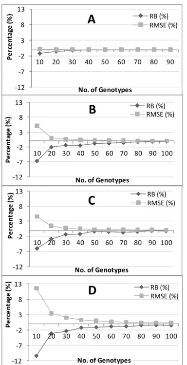
The results for the estimates of genotypic variance are shown in Figure 1. As indicated, the RB values were all close to zero for all of the sample sizes and the varieties studied. The RMSE values were smaller for the trials with a higher heritability and decreased as the sample size increased. These values increase from Fig. 1A to Fig. 1D (Tinta Miúda < Viosinho < Antão Vaz < Negra Mole). With a sample size of 10 genotypes, the RMSE ranged from 20% in the trial with Tinta Miúda to 45% in the trial with Negra Mole. When taking a sample size of 40 genotypes, the RMSE ranged from 3.1% for Tinta Miúda to 8.5% for Negra Mole. At a sample size of 60, the RMSE ranged from 1.4% for Tinta Miúda to

-5

5

15

25

35

45

10

20

30

40

50

60

70

80

90

Pe

rc

e

n

ta

ge

(%

)

No. of Genotypes

A

RB (%)

RMSE (%)

-5

5

15

25

35

45

10 20 30 40 50 60 70 80 90 100

Pe

rc

e

n

ta

ge

(%

)

No. of Genotypes

B

RB (%)

RMSE (%)

-5

5

15

25

35

45

10 20 30 40 50 60 70 80 90 100

Pe

rc

e

n

ta

ge

(%

)

No. of Genotypes

C

RB (%)

RMSE (%)

-5

5

15

25

35

45

10 20 30 40 50 60 70 80 90 100

Pe

rc

e

n

ta

ge

(%

)

No. of Genotypes

D

RB (%)

RMSE (%)

Fig. 1. Relative bias (RB) and relative mean square error (RMSE) for the genotypic variance estimates. A – Tinta Miúda; B – Viosinho; C – Antão Vaz; D – Negra Mole.

3.8% for Negra Mole. The differences between the RMSE values start to get very small with a sample size of 40 genotypes. When examining 60-70 genotypes, the differences are close to zero. Thus, the results obtained using 60-70 genotypes are nearly as good as those obtained using all of the genotypes in the trial.

The results for the estimates of broad-sense heritability are shown in Figure 2. As with the genotypic variance estimates, lower RMSE values were observed in the Tinta Miúda variety, and higher RMSE values were observed in the Negra Mole variety. The RMSE decreased as the sample size increased; however, this decrease became less marked with a sample size of 40 clones for all the studied varieties. Looking at the RB values, one can see that for sample sizes less than 40 the broad-sense heritability is underestimated, especially in the case of Negra Mole. From Figure 2, it is apparent that broad-sense heritability estimates obtained from samples with approximately 40 genotypes are close to those obtained with all of the genotypes in the trial; that is, the values of RB and RMSE obtained for the broad-sense heritability estimates are very close to zero.

In summary, the results for the estimates of broad-sense heritability indicated that estimates based on 40 clones showed approximately the same results as using all of the clones in the trial. However, the results obtained for the component of genotypic variance analysis are not so clear.

As this study is based on actual field trials, the quality of the estimates of the genotypic variance of the yield varied with the trial. The higher the heritability measurements obtained for the trial, the lower the number of genotypes that were required to obtain accurate estimates of the genetic variance. The results showed that the minimum number of genotypes needed to adequately represent the genetic variability of a variety ranged from 40 to 50 genotypes per growing region. However, at a sample size of approximately 70 genotypes, the quality of the estimates of genotypic variance started to become independent from the quality of the trial. From this number, the results obtained with all trials are the same, and therefore, a sample size of 70 will protect the analysis from less than favourable experimental conditions that may arise.

Now that we know the minimum number of genotypes, or parental plants, to integrate into the representative sample, the question of how to mark the plants in the vineyards and to ensure its representativeness remains. First, the set of marked plants must have a geographic distribution that is similar to the density distribution of old vines in the region that they are intended to represent. The restriction to the old vines means to prospect plants in vineyards that were planted prior to the existence of selection and nursery activities because only those preserve the diversity that was created in the past. The vineyards explored should be as geographically distant as possible and should not have be related (meaning the vineyards should have different owners, different years of planting, etc.). As a consequence, the total number of plants should come from the largest possible number of vineyards (20 or more), and only a few plants from each vineyard should be sampled (5 or less). Within each vineyard, the plants should be separated and must be marked in a casual way (except in cases of serious diseases of a systemic type).

2.2 Experimental designs suitable for large field trials

To quantify the genetic variation within a variety and to perform efficient selection, it is necessary to plant a very large field trial (normally between 100 and 400 clones), which will

-12

-7

-2

3

8

13

10

20

30

40

50

60

70

80

90

Pe

rc

e

n

ta

ge

(%

)

No. of Genotypes

A

RB (%)

RMSE (%)

-12

-7

-2

3

8

13

10 20 30 40 50 60 70 80 90 100

Pe

rc

e

n

ta

ge

(%

)

No. of Genotypes

C

RB (%)

RMSE (%)

-12

-7

-2

3

8

13

10 20 30 40 50 60 70 80 90 100

Pe

rc

e

n

ta

ge

(%

)

No. of Genotypes

D

RB (%)

RMSE (%)

-12

-7

-2

3

8

13

10 20 30 40 50 60 70 80 90 100

Pe

rc

e

n

ta

ge

(%

)

No. of Genotypes

B

RB (%)

RMSE (%)

Fig. 2. Relative bias (RB) and relative mean square error (RMSE) for the broad-sense heritability estimates. A – Tinta Miúda; B – Viosinho; C – Antão Vaz; D – Negra Mole.

contain a representative sample of the variability within the variety across the different regions in which it is grown. Thus, the initial field trials for a grapevine variety would cover an unusually large area (from 0.75 to 1.5 ha), which by itself can cause a large amount of environmental variation. Therefore, the importance of experimental design in this type of trial is crucial to quantify the genetic variability and successfully select a superior group of clones.

The most relevant experimental designs for working with a high number of treatments (greater than 100 genotypes) are the alpha designs (Patterson & Williams, 1976), the row-column designs (Williams & John, 1989), the t-latinised designs (John & Williams, 1998) and the resolvable spatial row-column designs (Williams et al., 2006). The use of these designs in initial trials of grapevines was studied by Gonçalves et al. (2010). In that work, the authors compared several experimental designs via simulations, including randomised complete block, alpha and row-column designs, with the aim of identifying the designs that are most suitable for quantifying and utilising the genetic variability. For these purposes, they concluded that the alpha and row-column designs were better than the randomised complete block (RCB) design.

2.3 A review of several mixed models that are used in data analysis from large grapevine field trials

The theory of mixed models was developed in recent years, has been applied to a wide scope of sciences (Searle et al., 1992; Pinheiro & Bates, 2000; Verbeke & Molenberghs, 2000; McCulloch & Searle 2001; Giesbrecht, & Gumpertz, 2004; Littell et al., 2006; Butler et al., 2009; Lawson, 2010) and forms the basis for data analysis from grapevine selection trials.

Generally in these models, the genotypic effects are considered to be random effects because a random sample of genotypes of the cultivated variety is studied. The spatial control is done with the factors of the experimental design and, when necessary, through the variance-covariance matrix of the vector of the errors. Examples of mixed spatial models that are applied to grapevine initial field trials are described in Gonçalves et al. (2007). Models for data analysis of different experimental designs, namely, models for the analysis of randomised complete block, alpha, row-column and latinised designs, are described in Gonçalves et al. (2010).

The general linear mixed model can be written as

  

y X



where y_n1 is the vector of observations, X_{n p } is the design matrix of fixed effects, _p1

is the vector of fixed effects, Z_{n q } is the design matrix of random effects, u_q1 is the vector of random effects and e_n1 is the vector of random errors.

The vectors, u and e , are assumed to be independent with a multivariate normal

distribution (MVN) with mean vector 0 and variance-covariance matrices, G_{q q } and

n n

R _ , respectively. The distribution of y is then multivariate normal with mean vector



T

V ZGZ  , R

whereZTdesignates the transposition of Z .

When several traits, generally uncorrelated ones, are evaluated, the vector of observations,

n 1

y _ , has the form





T T T T

t

y y y  y , and the vector of the random errors has the form





T T T T

t

e e e e ,

where t represents the number of the evaluated traits and, for example, y is a vector with 1 1

n observations for yield, y is a vector with ₂ n observations for ºBrix, etc., and ₂ e , ₁ e , ₂

etc., are the correspondent vectors of random errors.

The vector  contains the overall mean and other effects such as effects associated with experimental design, effects associated with the different growing regions of the variety when several regions are considered, the effects of different traits when several traits are studied, and so forth.

The vector u usually consists of k sub-vectors, such that





T T T

k

u u u , and the design matrix associated with the vector u , is given by





Z Z Z  Z ,

where Z Z1, 2, , Zk are the design matrices associated to random effects vectors 1, 2, , k

u u  u , respectively.

Therefore, to generalise to k random effect factors, Zu is decomposed as







Each random effects factor, represented by u , may represent the genotypic effects of a trait, _i

the effects associated with the experimental design of the trial, and so forth and has the properties

 

 





Consequently,

 

  _ik i

Var u G G ,

where _i2 is the variance of the random effects factor i , I is the q_i q q identity matrix, i i

and G is the direct sum of matrices G . _i

In the simplest formulation, it is assumed that the elements of the vector e are independent and identically distributed (iid) normal random variables, which leads to a variance-covariance matrix that is defined as

2  _{e n}

R  I , where _2

e is the variance of the error and I is the n n n identity matrix.

However, according to studies that have already been conducted in initial field trials with the grapevine (Gonçalves et al., 2007), the vector e often represents the sum of two vectors,

  . The components of the vector  are dependent from space, and it is assumed that





~MVN 0,

   , where _2 _{is the spatially dependent variance and }2_{0, and that } is a _{n n spatial correlation matrix, whose nondiagonal elements will be given by an} anisotropic power correlation function. The components of the vector  are iid random variables and ~MVN







n n identity matrix. Consequently, the variance-covariance matrix for the vector of the errors is defined as

2 2

  _n

R  I .

When block effects are assumed to be fixed, the spatial modelling is made block by block, and it is usually assumed to be equal for all blocks.

When several traits are considered to be uncorrelated, the matrix R takes the form

1   _it i

R R ,

where Ri is the error variance-covariance matrix for the trait i .

Obviously, this is only a short review of the possible models that can be applied to data analysis from grapevine initial selection trials, and many other models could be addressed. However, our objective was to introduce the methodology that will be applied in the examples that follow in sections 2.4 and 2.5. One of these is a model that incorporates a nested structure for the genotypic effects to quantify the genetic variability by the growing region. The other is a model that analyses several traits to quantify the genetic variability per trait. In both situations, an RCB design will be considered.

The first approach will be supported by a mixed model, where several genotypic variance components are estimated and each one corresponds to a growing region. When considering an RCB design, the following model can be used

( )

    

ijk i j ik ijk

y region block clone region e (1)

for 1, ,i  s , j 1, ,r and k 1, ,q , where i q is the number of genotypes in the region i

i . In the model, yijk represents the observation of the clone k of the region i in the block j, 

represents the overall mean, regioni represents the fixed effect of the region, block j

represents the random complete block effect or, depending on the trial, the fixed complete block effect, clone region( )ik represents the random genotypic effect within the region and e ijk

represents the random error associated to the observation yijk.

With regard to the second approach, the model simultaneously analyses several traits. It uses a mixed model approach in which several genotypic variance components are estimated, and each one corresponds to a trait. When considering an RCB design, the model for this analysis can be written as

( ) ( )

    

ijk i ij ik ijk

y trait block trait clone trait e (2)

for 1, ,i t ; j 1, ,ri, where ri is the number of blocks for the trait i ; and k 1, ,qi,

where qi is the number of genotypes evaluated for the trait i . In the model, yijk represents

the observation of the trait i in the clone k in the block j,  represents the overall mean,

i

trait represents the fixed effect of the trait, block trait represents the random complete





random error associated to the observation yijk.

2.4 Examples of quantification of genetic variability within ancient varieties

To study the intravarietal genetic variability, the cases of two Portuguese autochthonous grapevine varieties, Trincadeira and Síria, are given as example. The genotypes of Tricandeira were sampled in 4 regions (Alentejo, Oeste, Dão and Pinhel). The genotypes of Síria were sampled in 3 regions (Algarve, Alentejo and Pinhel). The field trials of Trincadeira and Síria were planted in Ribatejo and Pinhel, respectively, and both were laid out according to a randomised complete block design with 5 resolvable replicates and 4 plants per plot.

Data analysis was based on the average yield values observed over several years (1988, 1989 and 1990 for Trincadeira and 1988 and 1989 for Síria) and was performed using PROC MIXED of SAS version 9.2 (SAS Institute, 2008). For each variety, several mixed models were fitted to the yield data in order to address several relevant questions. The parameters involved in the model were estimated by residual maximum likelihood (REML) (Patterson & Thompson, 1971), using the Fisher Scores algorithm (Jennrich & Sampson, 1976).

The first question is to clarify if the varieties have significant genetic variability in the yield in Portugal. Thus, the first model that was fitted to the yield data was a model that considered all of the genotypes to be a sample from a single origin, Portugal. Additionally, the model assumed random block effects, used an anisotropic power function for the spatial correlated errors and a nugget effect (later called model A). A residual likelihood ratio test (REMLRT)

was used to test the null hypothesis that the genotypic variance component was equal to zero. Since the null hypothesis, which involves a variance component, was on the boundary of the parameter space, the p-value of the test was half of the reported p-value from the chi-squared distribution with one degree of freedom (Self & Liang, 1987; Stram & Lee, 1994).

However, as these varieties exist in different regions of Portugal, another important question is whether this genetic variability is equal for all regions or whether, on the contrary, it differs according to region. To answer this question, two models that considered the origin of the genotypes by region of Portugal were fitted. One model assumed an equal genotypic variances for all of the regions and was later referred to as model B. The other assumed an unequal genotypic variances among the regions and was later referred to as model C. In both models, growing region effects were considered as fixed, block effects were considered as random and, for the random errors, an anisotropic power function for the spatial correlated errors and a nugget effect were considered.

A REMLRT was used to compare the fit of model B with the fit of model C. The distribution of the REMLRT statistic was considered to be a chi-squared with three degrees of freedom to compare models B and C in Trincadeira and with two degrees of freedom when comparing the models in Síria. These models were also compared using the Akaike’s Information Criterion (AIC) and the Bayesian Information Criterion (BIC), and for these criteria, smaller values indicate a better fit.

To develop a better understanding of the amount of genetic variability between regions of the variety and between the varieties themselves, the coefficient of genotypic variation (the ratio between the estimate of the genotypic standard deviation and the estimate of the overall mean) was also computed.

The results for the quantification of the genetic variability of yield without taking into account the factor region (model A) are illustrated in Table 2. The genotypic variance was highly significant for both varieties. The REMLRT statistics ((-2lR0) - (- 2lR))were 174.6 with a

p -value<0.0001 for Trincadeira, and 352.2 with a p-value<0.0001 for Síria. When comparing the genetic variability of the yield between varieties under the experimental conditions studied, it was noted that Síria had a higher degree of genetic variability than Trincadeira. This conclusion can be more easily perceived through the values for CVG, which were 26.0%

for Síria and 15.3% for Trincadeira. These indicators point to a greater antiquity of Síria in Portugal compared with Trincadeira.

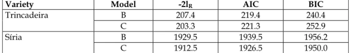
To compare the genetic variability within the variety in different growing regions, models B and C were fitted, and the results for minus twice the residual log-likelihood, AIC and BIC, are listed in Table 3.

Variety No. of Genotypes 2 ˆ _g -2lR -2lR0 ˆ CVG (%) Trincadeira 246 0.025 211.7 386.3 1.030 15.3 Síria 210 0.251 1955.4 2307.6 1.930 26.0

Table 2. Estimates of the overall mean ( ˆ), the genotypic variance (_ˆ2

g) and the coefficient

of genotypic variation (CVG), the minus twice the residual log-likelihood (-2lR) obtained with

the fitting of model A and the minus twice the residual log-likelihood obtained with a variant of the model A without genotypic effects (-2lR0).

Variety Model -2lR AIC BIC

Trincadeira B 207.4 219.4 240.4

C 203.3 221.3 252.9

Síria B 1929.5 1939.5 1956.2

C 1912.5 1926.5 1950.0

Table 3. Minus twice the residual log-likelihood (-2lR), Akaike’s Information Criterion (AIC)

and Bayesian Information Criterion (BIC) obtained from the fitting of models B and C. For Trincadeira, the observed value for the REMLRT statistic ((-2lRB)-(-2lRC)) was 4.1 with a

p-value of 0.2508. Consequently, the null hypothesis of equal genotypic variances of yield was not rejected, indicating that the equal variance model (model B) is adequate to describe the data. The superiority of model B was also confirmed by the lower values obtained for the AIC and the BIC (219.4 and 240.4, respectively).

On the contrary, the null hypothesis of equal genotypic variances of yield among the regions of Alentejo, Algarve and Pinhel was rejected for Síria. In fact, the observed value for the REMLRT statistic ((-2lRB)-(-2lRC)) was 17with a p-value of 0.0002. Additionally, on the basis

of the AIC and the BIC, the unequal variance model (model C) was better than model B. The values obtained for these criteria were, respectively, 1926.5 and 1950.0 for model C, and 1939.5 and 1956.2 for model B.

In fact, observing the differences between the genotypic variance estimates for the different regions and the corresponding values of the CVG, the differences were more

marked in Síria (Table 4). The yield genotypic variances are quite different, ranging from 0.060 in Alentejo to 0.291 in Pinhel, which corresponds to values of 11.2% and 32% for the CVG, respectively.

Variety Region _Genotypes No. of ˆ _ˆ2

g CVG (%) Trincadeira Alentejo 55 1.058 0.025 14.9 Oeste 61 0.961 0.030 18.0 Dão 87 1.083 0.020 13.1 Pinhel 43 0.984 0.013 11.6 Síria Algarve 78 2.031 0.217 23.0 Alentejo 49 2.184 0.060 11.2 Pinhel 83 1.683 0.291 32.0

Table 4. Estimates of the overall mean ( ˆ), genotypic variance (_ˆ2

g) and coefficient of

genotypic variation (CVG) obtained with the fitting of model C to the yield data (kg/plant).

To compare the antiquity of the varieties, it is more important to understand the variability of each one on its more heterogeneous region than to know the total average variability. On the basis of this criterion, the higher genetic variability of the Síria variety is also confirmed if we look to the CVG obtained for the regions with a higher genetic variability (Table 4).

That is, Síria in the Pinhel region had a CVG of 32% and Trincadeira in the Oeste Region had

a CVG of 18%. Once again, these indicators reinforce the greater antiquity of Síria compared

To summarise, for Trincadeira, the genetic variability of the yield was equal in all regions. Trincadeira is a greatly expanded variety in Portugal, and it is likely that the constant exchange of material among the regions homogenised this variability.

For Síria, the greatest genetic variability was was found in the Pinhel region. This finding may indicate that the variety originated in Pinhel. Then, it was exported to the other regions, likely through selected material. This is logical, as the region with the highest genetic variability is the one that shows the lowest mean yield. When performing multiple pairwise comparisons of the means, the adjusted p-values indicated that the mean yield for Pinhel is lower than the means for Algarve and Alentejo (p-values<0.05). Likely, the exportation of the variety to other regions occurred only once. If they were several exports then the variability would tend to be equal in all regions as in the case of Trincadeira.

2.5 Examples of mass genotypic selection for important traits

The examples for mass genotypic selection will be conducted in another two Portuguese varieties, Arinto and Vital. The trial of Arinto was located in Setúbal and was laid out in a randomised complete block design with 247 genotypes, 4 plants per plot and 4 complete blocks. The traits considered for this study were yield (kg/plant) in 1995, 1998, 1999 and 2000 and soluble solids (ºBrix) in 2005 and 2006. The trial with Vital was located in Caldas da Rainha and was laid out in a randomised complete block design with 232 genotypes, 4 plants per plot and 4 complete blocks. The traits considered were yield (kg/plant) in 1990, 1991 and 1992 and soluble solids (ºBrix) in 1992. Because of the feasibility of evaluating the soluble solids, samples of 60 berries were collected by plot in the 3 most homogenous blocks. The analysis of the grape berries for evaluation of soluble solids was made following standard laboratory techniques.

Once again, the theory of mixed models and REML estimation were used and mixed model 2 of section 2.3, which assumed the block was fixed, was fitted to the data using PROC MIXED of SAS version 9.2 (SAS Institute, 2008). For Arinto, an anisotropic power function for correlated errors and a nugget effect were considered. For Vital, only independent and identically distributed errors were assumed. For both varieties the traits analysed were assumed to be uncorrelated. This decision was supported by previously descriptive analysis, which provided a Pearson’s correlation coefficient between the traits of 0.11 for Arinto, and -0.17 for Vital.

After fitting the mixed models to the yield and ºBrix data, the empirical best linear unbiased predictors (EBLUPs) of genotypic effects of those traits were obtained through the mixed model equations (Henderson, 1975; Searle et al., 1992). A generalised t-test (McLean & Sanders, 1988; Kenward & Roger, 1997) was performed to test the null hypothesis that the genotypic effect of a trait in a clone was equal to zero. The prediction standard errors were adjusted according to Prasad & Rao (1990) and Harville & Jeske (1992).

The EBLUPS of the genotypic effects were used to select clones and two distinct groups of clones from each variety were selected according to the trait. That is, two types of mass genotypic selections were made, one with the best clones for yield and the other with the best clones for ºBrix.

The predicted genetic gain to be obtained through the selection of those groups was computed as the average of the EBLUPs of the respective genotypic effects. To better interpret the results, the predicted genetic gain was expressed as a percentage of the overall mean.

The results for the mass genotypic selection are shown in Table 5. The genotypic variance component was statistically significant (p-value<0.0001) for the two analysed traits for both varieties (the statistical test was the same as described in the previous section). This result indicates that there is sufficient “raw material” (genetic variability) to apply selection. For a selection of top 15% of the genotypes, the predicted genetic gains of yield were 32.1% and 43.1% for Arinto and Vital, respectively. For the ºBrix, the predicted genetic gains were 10% for Arinto and 10.8%, for Vital. For Arinto, all of the genotypes in the group selected for yield showed a significant genotypic effect (p-value<0.05), and the genotypic effect of the last clone of the group was significant with a p-value of 0.0167. The ºBrix group also had significant genotypic effects for all of the clones (p-value<0.05). The genotypic effect of the last clone of the group was significant with a p-value of 0.0024. For Vital, all of the genotypes in the group selected for yield showed a significant genotypic effect (p-value<0.05), and the genotypic effect of the last clone of the group was significant (p-value=0.0485). However, in the group selected for ºBrix, four of the clones did not reveal a significant genotypic effect (p-value>0.05). This result indicates that the efficiency of selection is not equal in the two varieties and is higher in the Arinto variety.

Variety Trait _ˆ2

g

 p-value _{selection of 15% of the superior genotypes} Predicted genetic gain (%) obtained by

Arinto Yield (kg/plant) 0.1283 <0.0001 32.1% Soluble solids (ºBrix) 2.7497 <0.0001 10.0% Vital Yield (kg/plant) 0.3361 <0.0001 43.1%

Soluble solids (ºBrix) 2.4941 <0.0001 10.8% Table 5. The genotypic variance estimates for yield and ºBrix ( _ˆ2

g

 ) and the predicted genetic gains obtained with selection proportion of 15% for the two studied varieties.

One issue remains to be clarified: why perform mass genotypic selection instead of using clonal selection?

To answer this question, we use a short demonstration. A group with the 30 top genotypes for yield was selected for each variety on the basis of the analysis of the mean yield for several years. The predicted genetic gain for this group of genotypes was computed separately year by year. In parallel, three individual top genotypes were selected for yield, also based on the mean yield of several years. Again, their behaviour was evaluated for individual years. The results are reported in Table 6.

For Arinto, the predicted genetic gain in the group of 30 clones is more stable over the years, ranging from 31.8% to 32.2%, than the behaviour of the individual clones. The clone, AR4108, always remained above the group of 30 genotypes and the genotypic effects of yield were always significantly different from zero (p-value<0.05). However, other genotypes did not always show a yield above the selected group, and their yield genotypic effects were not significant (p-value>0.05) for some years. The AR3605 clone in 1998 and the AR3903 clone in 2000 are two examples of this occurrence.

Variety/clone Year EBLUP p-value % of yield above

the overall mean

Arinto/AR4108 1998 0.776 0.0009 46.9 1999 0.872 <0.0001 51.6 2000 0.847 <0.0001 68.3 Arinto/AR3605 1998 0.403 0.0839 24.4 1999 0.787 0.0002 46.5 2000 1.190 <0.0001 96.0 Arinto/AR3903 1998 0.686 0.0034 41.5 1999 0.663 0.0018 39.2 2000 0.288 0.1261 23.2 Arinto/Group 1998 0.529 32.0 1999 0.537 31.8 2000 0.400 32.2 Vital/VT1402 1990 0.441 0.0067 83.0 1991 0.373 0.4336 16.3 1992 1.653 <0.0001 70.7 Vital/VT1218 1990 -0.061 0.7055 -11.5 1991 1.297 0.0067 56.7 1992 1.251 0.0026 53.5 Vital/VT1208 1990 0.152 0.3475 28.6 1991 1.352 0.0047 59.1 1992 1.027 0.0133 43.9 Vital/Group 1990 0.200 37.7 1991 0.818 35.7 1992 0.929 39.7

Table 6. Behaviour of the group of clones and individual clones with respect to yield over the years compared on the basis of the empirical best linear unbiased predictors (EBLUPs) of the genotypic effects of yield and of the percentage of the yield above the overall mean. For the group, EBLUP is the average of the EBLUPS of the genotypic effects of the yield of the correspondent clones.

For Vital, the predicted genetic gain with the group of 30 clones was also more stable, ranging from 35.7% to 39.7%, than the behaviour of individual clones. The genotypic effects on the yield of the VT1218 and VT1208 clones were not significant (p-value>0.05) in 1990. In that year, these genotypes revealed a yield below the group of clones. In 1991, the VT1402 clone had a lower yield than the group of clones, and the yield genotypic effect was not significant (p-value>0.05).

To summarise, the results clearly indicate the difference between the behaviour of a group of clones and an individual clone. With a group of clones or with mass genotypic selection, the predicted genetic gains of yield remain nearly constant over the years considered. In contrast, the individual clones showed a more unstable behaviour. There were clones that appeared to be more stable, for example, the AR4108 clone. However, the sample of the evaluated environments is not sufficiently representative to make a more objective

interpretation. This phenomenon that we are referring to is nothing more than the genotype×environment interaction. Because of this phenomenon, and to minimise its negative effects, reliable clonal selection requires the installation of numerous regional trials and data collection for several traits over a number of years. This process has at least two highly negative consequences, the costs become very cumbersome and may derail the selection work and the objectives formulated at the beginning of selection may already be outdated when it is completed 10-15 years later. Clonal selection is more time consuming and more expensive than mass genotypic selection. The option of selecting groups of clones from the initial field trial is cheaper than clonal selection, preserves some genetic variability of the variety in vineyards and it is a good strategy for overcoming genotype×environment interactions.

3. Conclusion

This chapter focused on the study of ancient grapevine varieties. Indeed, only ancient varieties can have enough intravarietal genetic variability to ensure the success of the presented methodologies.

The analyses were directed to situations in which we do not have any prior knowledge on the genetic variability within the varieties. Therefore, the approach was based on methods that, when properly articulated, can simultaneously respond to three key issues: (1) quantification and knowledge on geographical distribution of intravarietal variability, (2) selection of a high performance group of genotypes and (3) conservation of genetic variability and halting genetic erosion.

The main conclusions cover 3 important points.

1. The results on sampling of variability showed that the minimum number of genotypes needed to adequately represent the genetic variability of a variety ranges from 40 to 50 genotypes per growing region.

2. It was shown that there are high levels of genetic variability in two of the most important traits of grapevine and that those levels are different in different varieties and in different growing regions of the same variety.

3. Mass genotypic selections for two of the most important traits were successfully performed. This methodology is defended as a cheap, fast and efficient selection procedure and has the additional advantage of minimizing the genotype×environment interaction.

4. Acknowledgment

We are grateful to our colleagues of ‘‘National Network for Grapevine Selection’’ for their help in data collection. This work was funded by “Fundação para a Ciência e Tecnologia, Portugal” (BPD/43218/2008; PEst-OE/AGR/UI0240/2011).

5. References

Arroyo-García, R.; Ruiz-García, I.; Bolling, L.; Ocete, R.; López, M.A.; Arnold, C.; Ergul, A.; Söylemezoglu, G.; Uzun, H.I.; Cabello, F.; Ibáñez, J.; Aradhya, M.K.; Atanassov, A.; Atanassov, I.; Balint, S.; Cenis, J.L.; Costantini, L.; Gorislavets, S.; Grando, M.S.; Klein,

B.Y.; McGovern, P.E.; Merdinoglu, D.; Pejic, I.; Pelsy, F.; Primikirios, N.; Risovannaya, V.; Roubelakis-Angelakis, K.A.; Snoussi, H., Sotiri, P.; Tamhankar, S.; This, P.; Troshin, L.; Malpica, J.M.; Lefort, F. & Martinez-Zapater, J. M. (2006). Multiple origins of cultivated grapevine (Vitis vinifera L. ssp. sativa) based on chloroplast DNA polymorphisms. Molecular Ecology, Vol.15, No.12, pp. 3707-3714, ISSN 1365-294X Butler, D.; Cullis, B.; Gilmour, A. & Gogel, B. (2009). Mixed models for S language

environments, ASReml-R reference manual. The Department of Primary Industries and Fisheries (DPI&F), ISSN 0812-0005, Queensland, Australia

Falconer, D. & Mackay, T. (1996). An introduction to quantitative genetics. 4th edn.. Prentice Hall, ISBN 0582-24302-5, London, United Kingdom

Giesbrecht, F. & Gumpertz, M. (2004). Planning, construction, and statistical analysis of comparative experiments. John Wiley & Sons Inc., ISBN 0-471-21395-0, Hoboken, New Jersey, USA

Gonçalves, E.; St.Aubyn, A. & Martins, A. (2007). Mixed spatial models for data analysis of yield on large grapevine selection field trials. Theor Appl Genet, Vol.115, No.5, pp.653-663, ISSN 1432-2242

Gonçalves, E.; St.Aubyn, A. & Martins, A. (2010). Experimental designs for evaluation of genetic variability and selection of ancient grapevine varieties: a simulation study. Heredity, Vol.104, No. 6, pp. 552-562, ISSN 0018-067X

Harville, D. & Jeske, D. (1992). Mean squared error of estimation or prediction under a general linear model. J Am Stat Assoc, Vol.87, No.419, pp. 724-731, ISSN 0162-1459 Henderson, C. (1975). Best linear unbiased estimation and prediction under a selection

model. Biometrics, Vol.31, No.2, pp. 423-447, ISSN 1541-0420

Jennrich, R. & Sampson, P. (1976). Newton-Raphson and related algorithms for maximum likelihood variance component estimation. Technometrics, Vol.18, No.1, pp. 11-17, ISSN 1537-2723

John, J. & Williams, E. (1998). t-Latinized designs. Aust Nz J Stat, Vol.40, No.1, pp. 111-118, ISSN 1467-842X

Kenward, M. & Roger, J. (1997). Small sample inference for fixed effects from restricted maximum likelihood. Biometrics, Vol.53, No.3, pp. 983-997, ISSN 1541-0420

Laucou, V.; Lacombe, T.; Dechesne, F.; Siret, R.; Bruno, J.-P.; Dessup, M.; Dessup, T.; Ortigosa, P.; Parra, P.; Roux, C.; Santoni, S.; Vares, D.; Peros, J.-P.; Boursiquot, J.-M. & This, P. (2011). High throughput analysis of grape genetic diversity as a tool for germplasm collection management. Theor Appl Genet, Vol.122, No.6, pp. 1233-1245, ISSN 1432-2242 Lawson, J. (2010). Design and Analysis of Experiments with SAS. Champman & Hall, CRC,

ISBN 978-1-4200-6060-7, New York, USA

Littell, R.; Milliken, G.; Stroup, W.; Wolfinger, R. & Schabenberger, O. (2006). SAS system for mixed models. 2nd edn.. SAS Institute, ISBN 978-1-59047-500-3, Cary, NC, USA Lynch, M. & Walsh, B. (1998). Genetics and analysis of quantitative traits. Sinauer Associates,

Inc., ISBN 0-87893-481-2, Sunderland, United Kingdom

Martins, A. (2007). Variabilidade genética intravarietal das castas. In: Portugal vitícola, o grande livro das castas, J. Böhm, (Ed.), 53-56, Chaves Ferreira Publicações, ISBN 9728987102, Lisboa, Portugal

Martins, A. (2009). Genetic diversity of portuguese grapevines: methods and strategies for its conservation, evaluation and conservation. Acenología, No. 112, Available from

http://www.acenologia.com/cienciaytecnologia/variedades_portuguesas_cien120 9.htm

Martins, A.; Carneiro, L. & Castro, R. (1990). Progress in mass and clonal selection of grapevine varieties in Portugal. Vitis, special issue, pp. 485-489, ISSN 0042-7500 Martins, A.; Carneiro, L.; Gonçalves, E. & Eiras-Dias, J. (2006). Methodology for the analysis

and conservation of intravarietal variability: the example of grapevine cv Aragonez, Proceedings of XXIX Congress of OIV, ISSN: 251-06-001-9, Logroño, Spain, June 25-30, 2006

McCulloch, C. & Searle, S. (2001). Generalized linear and mixed models. John Wiley & SonsInc., ISBN 0-471-19364-x, New York, USA

McLean, R. & Sanders, W. (1988). Approximating degrees of freedom for standards errors in mixed linear models, Proceedings of the Statistical Computing Section, American Statistical Association, pp. 50-59, New Orleans, USA

Myles, S.; Boyko, A.; Owens, C.; Brown, P.; Grassi, F.; Aradhya, B.; Reynolds, A.; Chia, J.; Ware, D.; Bustamante, C. & Buckler, E. (2011). Genetic structure and domestication history of the grape. PNAS, Vol.108, No.9, pp. 3530-3535., ISSN 1091-6490

Patterson, H. & Thompson, R. (1971). Recovery of inter-block information when block sizes are unequal. Biometrika, Vol.58, No.3, pp. 545-554, ISSN 1464-3510

Patterson, H. & Williams, E. (1976). A new class of resolvable incomplete block designs. Biometrika, Vol.63, No.1 , pp. 83-92, ISSN 1464-3510

Pelsy, F.; Hocquigny, S.; Moncada, X.; Barbeau, G.; Forget, D.; Hinrichsen, P. & Merdinoglu, D. (2010). An extensive study of the genetic diversity within seven French wine grape variety collections. Theor Appl Genet, Vol.120, No.6, pp. 1219-1231, ISSN 1432-2242 Pinheiro, J. & Bates, D. (2000). Mixed-effects models in S and S-plus. Springer-Verlag, ISBN

978-1-4419-0317-4, New York, USA

Prasad, N. & Rao, J. (1990). The estimation of the mean squared error of small-area estimators. J Am Stat Assoc, Vol.85, No.409, pp. 163-171, ISSN 0162-1459

SAS Institute Inc. (2008). SAS/STAT® 9.2 User’s Guide. SAS Institute Inc., ISBN 978-1-59047-949-0, Cary, NC, USA

Searle, S.; Casella, G. & McCulloch, C. (1992). Variance components. John Wiley & Sons Inc., ISBN 13-978-0-470-00959-8, Hoboken, New Jersey, USA

Sefc, K.M.; Lefort, F.; Grando, M.; Steinkellner, H. & Thomas, M. (2001). Microsatellite markers for grapevine: a state of the art. In: Molecular biology biotechnology of grapevine, K.A. Roubelakis-Angelakis, (Ed.), 433-463, Kluwer Publishers, ISBN 0-7923-6949-1, Amsterdam, Netherlands

Self, S. & Liang, K. (1987). Asymptotic properties of maximum likelihood estimators and likelihood ratio tests under nonstandard conditions. J Am Stat Assoc, Vol.82, No.398, pp. 605–610, ISSN 0162-1459

Stram, D. & Lee, J. (1994). Variance components testing in the longitudinal mixed effects model. Biometrics, Vol.50, No.4 , pp. 1171–1177, ISSN 1541-0420

Verbeke, G. & Molenberghs, G. (2000). Linear mixed models for longitudinal data. Springer-Verlag, ISBN 0-387-95027-3, New York, USA

Wiliams, E. & John, J. (1989). Construction of row and column designs with contiguous replicates. Appl Stat, Vol.38, No.1, pp. 149-154, ISSN 1467-9876

Williams, E.; John, J. & Whitaker, D. (2006). Construction of resolvable spatial row-column designs. Biometrics, Vol.62, No.1 , pp. 103-108, ISSN 1541-0420