Delvan Alves da Silva(1), Fabyano Fonseca e Silva(1), Henrique Torres Ventura(2), Vinícius Silva Junqueira(1), Alessandra Alves da Silva(1), Rodrigo Reis Mota(3) and Paulo Sávio Lopes(1)
(1)Universidade Federal de Viçosa, Departamento de Zootecnia, Avenida P.H. Rolfs, s/no, Campus Universitário, CEP 36570-000 Viçosa, MG,
Brazil. E-mail: [email protected], [email protected], [email protected], [email protected], [email protected] (2)Associação Brasileira dos Criadores de Zebu, Praça Vicentino Rodrigues da Cunha, no 110, Parque Fernando Costa,
CEP 38022-330 Uberaba, MG, Brazil. E-mail: [email protected] (3)Gembloux Agro-Bio Tech, Université de Liège, Passage des
Déportés, 2 B-5030 Gembloux, Belgium. E-mail: [email protected]
Abstract – The objective of this work was to evaluate the criteria for the formation of contemporary groups (CGs) in the genetic evaluation of body weight at weaning in Nellore cattle. A total of 713,474 records from 3,066 herds located in Midwestern and Northern Brazil were used. Data were obtained from the genealogical registry of zebu breeds of the Brazilian association of zebu breeders. Data structures were defined based on the number of standard deviations (SDs) for outlier removal (±2.0, ±2.5, ±3.0, and ±3.5) and on the minimal number of animals per CG (3, 7, and 15). Genetic evaluation was performed with an animal model using Bayesian inference. Data structures with ±3.5 SDs and CG with at least 15 animals presented the highest additive genetic variance (82.65±2.93), and those with ±2.0 SDs and CG with at least 3 animals showed the lowest one (60.23±1.96). The proper formation of CGs results in better-quality data archives, allowing to obtain more trustable estimates for the genetic parameters. Better selection responses are obtained when the following criteria are adopted for the removal of outliers: 2.5, 3.0, and 3.5 standard deviations and a minimum of 15 animals per contemporary group.
Index terms: heritability, outliers, zebu.
Grupos de contemporâneos na avaliação genética
de gado Nelore por inferência bayesiana
Resumo – O objetivo deste trabalho foi avaliar os critérios para formação de grupos de contemporâneos (GCs) na avaliação genética de peso ao desmame em bovinos Nelore. Foram utilizados 713.474 registros de 3.066 rebanhos localizados no Centro-Oeste e no Norte do Brasil. Os dados foram provenientes do Serviço de Registro Genealógico das Raças Zebuínas da Associação Brasileira dos Criadores de Zebu. As estruturas de dados foram definidas com base no número de desvios-padrão (DPs) para remoção de outliers (±2,0, ±2,5, ±3,0 e ±3,5) e no número mínimo de animais por GC (3, 7 e 15). A avaliação genética foi realizada por meio de modelo animal via inferência bayesiana. As estruturas de dados com ±3,5 DPs e GC com mínimo de 15 animais apresentaram a maior variância genética aditiva (82,65±2,93), e aquelas com ±2,0 DPs e GC com mínimo de 3 animais, a menor (60,23±1,96). A formação correta de GCs resulta em arquivos de dados mais consistentes, o que permite obter estimativas mais confiáveis dos parâmetros genéticos. As melhores respostas à seleção são obtidas ao se adotar os seguintes critérios para remoção de outliers: 2,5, 3,0 e 3,5 desvios-padrão e mínimo de 15 animais por grupo de contemporâneos.
Termos para indexação: herdabilidade, outliers, zebu.
Introduction
In the genetic evaluation of beef cattle,
non-genetic factors have been identified as important
sources of variation and may include: herd; year of birth; month of birth; nutritional, reproductive, and sanitary managements; and sex of the animal. These factors can be combined to form contemporary groups
(CGs), which, in a statistical model, allow removing the effects of environment and of different animal managements, in order to evaluate the expression of animal phenotypes under the same environmental conditions (Cobuci et al., 2006).
the homogeneity within the CG, which results in a smaller number of animals per group. Therefore,
the strategies used to define the CG might affect the
prediction accuracy of the expected differences among progenies. The incorrect formation of CGs leads to incorrect decision making, which, in turn, leads to the prediction of both overestimated and underestimated genetic values, respectively, for animals favored in the CG and subjected to less favorable conditions to express their genetic potential (Cobuci et al., 2006).
Outlier removal based on phenotypic standard deviation (SD) can be used in genetic evaluation for data consistency. However, the number of SDs for outlier removal is determined empirically in genetic
evaluations and there are no robust scientific studies on
CG formation that indicate the most adequate number to maximize the accuracy of genetic values.
In Brazil, there is still no agreement in the literature on the use of SDs for outlier removal and on the minimum number of animals per CG for the genetic evaluation of Nellore cattle. Bignardi et al. (2011), Shiotsuki et al. (2012), and Ferriani et al. (2013), for example, used ± 3.5 SDs and a minimum of 9, 3, and 4 animals per CG, respectively; Pedrosa et al. (2010), Matos et al. (2013), Santos et al. (2012), and Ambrosini et al. (2014), respectively, adopted ± 3.0 SDs and a minimum of 3, 7, 4, and 5 animals per CG.
The objective of this work was to evaluate the criteria for the formation of CGs in the genetic evaluation of body weight at weaning in Nellore cattle.
Materials and Methods
The weaning weights of 713,474 Nellore cattle, aged between 165 and 255 days, standardized to 210 days (W210), were recorded from 1993 to 2014. This data set is originated from 3,066 herds raised in the Midwestern and Northern regions of Brazil, and is included in the genealogical registry of the Brazilian association of zebu breeders.
For data consistency, records on the following animals were removed: offspring and parents with
similar identification; bulls and cows less than
609 days old at calving time; cows over 25 years old at calving; siblings with age difference less than 315 days; and animals derived from embryo transfer or in vitro fertilization techniques.
Birth months were grouped into four seasons: from November and December of the previous year to January of the following year; from February to April; from May to July; and from August to October. Three breeding conditions were assessed: pre-weaning animals, weaning animals, and animals subjected to weight-gain tests. Regarding feeding management, animals were raised in extensive pasture,
semi-confinement, and confinement. Cow age at calving
was grouped into 14 classes: class 1, containing 1.15% of the animals, corresponded to cows with less than 30 months of age at calving; classes 2 to 13 were formed for every 12-month interval, starting at 30 months of age; and class 14, containing 2.31% of the animals, grouped cows over 174 months of age at calving. Classes 2 (15.82%) and 3 (13.18%) presented the highest percentage of animals; both were combined with the factor sex of the animals and included as a qualitative systematic (non-genetic) effect in the model.
The CGs were formed considering herd, breeding condition, feeding management, sex, weighing date, year and season of birth. The CG was also included as a qualitative systematic effect in the model, whereas the age of the animal at weighing was considered as a quantitative systematic (linear and quadratic) effect.
Different criteria were assumed for outlier removal
in each CG. The first criterion was comparing the SD
to the mean (2.0, 2.5, 3.0, and 3.5) in each CG, and the second one was the removal of the CGs with less than 3, 7, and 15 animals. By merging these two criteria, 12 different data sets (E1 to E12) were generated (Table 1). Data consistency and editing were performed by the R software (The R Foundation, 2011).
Connectedness was determined for each data set,
previously defined according to the total number of
direct genetic links. This number was calculated based on the number of offspring from bulls and cows in common among the CGs, using the AMC software (Roso et al., 2004).
For the genetic evaluation, a single-trait animal model was used. Under matrix notation, this model can be described as follows:
y = Xb+Z a+Z m+Z pm+e
1 2 3 , in which
y
is the vector of the phenotypic observations on individual animals;
b
is the vector of systematic effects;
a
is the vector of direct additive genetic random effects;
m
is the vector of maternal additive genetic random effects;pm
is the vector of maternal permanent environmental random effects;
vector of residual effects; and X, Z1, Z2, and Z3 are the
incidence matrices that relate the observations to the systematic, direct additive genetic, maternal additive genetic, and maternal permanent environmental
effects, respectively. This model was fitted by Bayesian
inference, assuming probability distributions for data and unknown parameters according to Sorensen & Gianola (2002).
The conditional distribution of y, given the parameters, was assumed to be:
y
|
b
,
a
,
m
,pm
, G, σ σpm e b + Z a1 m+Z pm3
2 2
2
, ∼ ( , )
ɶ ɶ ɶ ɶ
N X +Z R and the residual
(co)variance matrix is R= σI e2
, in which I is an identity
matrix; N is the multivariate normal distribution, with mean and covariance assumed between parentheses; and G = A⊗G0, in which A is the numerator relationship
matrix of Wright’s coefficients and G0 is the additive
genetic covariance matrix.
For the systematic effects, it was assumed that: b ~ N(b0,V0), in which V0 is the non-informative
diagonal variance matrix, assuming V0 → 1010.
The direct and maternal additive genetic effects were assumed as:
ɶ ɶ
∼ a
m N G G A G G
a m = ⊗
0
0
G ( , );0 ; ,
0 0 0 2 2 σ σ
in which σa
2 is the direct additive genetic variance; σ m 2
is the maternal additive genetic variance; and G, G0,
and A have been previously described. The covariance between these genetic effects was assumed to be zero, based on the results reported by Mallinckrodt
et al. (1995), who suggested that possible negative genetic correlations between
a
and
m
may result in less accurate genetic predictions rather than in null correlations.The maternal permanent environmental effect was
assumed as:
pm
|σpm2 ~N (0, Iσ pm
2 ), in which σ pm 2 is the
maternal permanent environmental variance.
The scaled inverse chi-squared distribution was assumed for σpm
2
and σe 2
, with their respective densities. For the residual and maternal permanent environmental variances, the following distribution was used:
σe Seχve
2 2 2
−
and σpm Spmχvpm 2 2 −2
, in which S2
e = 194 and
S2
pm = 60, based on the variance estimates previously
reported in literature for W210; and ve = vpm = 5 is the
degree of confidence for these values.
The scaled inverse-Wishart distribution (IW2) was
assumed for G0, G0 ~ IW2 (∑, va), so that
162 5 0
0 40 .
∑
is the covariance matrix between direct and maternal
additive genetic effects, defined according to the
literature for W210; and va = 5 is the degree of
confidence for these values.
Bayesian inference was performed by Monte Carlo methods via Markov chains, using the GIBBS2F90 software (Misztal et al., 2014), which was run for a total of 500,000 iterations, after a burn-in period of 50,000 iterations. Samples were generated every 10
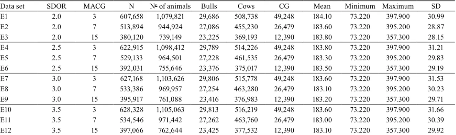
Table 1. Description of the evaluated data sets (E1 to E12), according to the standard deviations around the mean for outlier removal (SDOR), as well as minimum number of animals per contemporary group (MACG), number of observations (N), number of animals in the data archive, number of contemporary groups (CGs), means in kilograms, minimum and maximum values, and SD for weight at 210 days of age, in Nellore cattle(1).
Data set SDOR MACG N No of animals Bulls Cows CG Mean Minimum Maximum SD
E1 2.0 3 607,658 1,079,821 29,686 508,738 49,248 184.10 73.220 397.900 30.99 E2 2.0 7 513,894 944,924 27,086 455,230 26,479 183.60 73.220 395.200 28.87 E3 2.0 15 380,120 739,149 23,225 369,193 12,390 183.80 73.220 357.300 28.15 E4 2.5 3 622,915 1,098,412 29,789 514,226 49,248 183.80 73.220 397.900 31.21 E5 2.5 7 529,133 964,501 27,228 461,535 26,479 183.30 73.220 395.200 29.83 E6 2.5 15 392,031 755,646 23,376 375,017 12,390 183.50 73.220 357.300 29.19 E7 3.0 3 627,168 1,103,626 29,806 515,778 49,248 183.60 73.220 397.900 31.53 E8 3.0 7 533,386 969,957 27,254 463,280 26,479 183.10 73.220 395.200 30.23 E9 3.0 15 395,917 761,088 23,416 376,983 12,390 183.20 73.220 357.300 29.71 E10 3.5 3 628,328 1,105,063 29,813 516,219 49,248 183.60 73.220 397.900 31.66 E11 3.5 7 534,546 971,442 27,262 463,760 26,479 183.00 73.220 395.200 30.39 E12 3.5 15 397,066 762,644 23,425 377,532 12,390 183.10 73.220 357.300 29.92
iterations (thin = 10), resulting in a total of 45,000 effective samples for inference. The convergence was checked by visual inspection of trace plots and by Geweke’s Z criterion (Geweke, 1992).
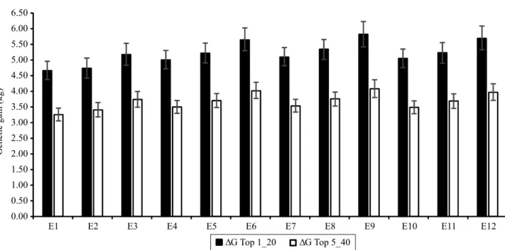
The genetic gains for different data sets were calculated by multiplying heritability (h2) and the
selection differential. The latter is the difference between the mean of the selected animals and of the entire population, with the selection of 1% of the best bulls and 20% of the best cows (Top 1_20) or of 5% of the best bulls and 40% of the best cows (Top 5_40).
The criteria for CG formation were evaluated and compared considering the percentage of common animals (ranking coincidence), according to the predicted breeding values, the differences in variance components and in genetic parameters, and the genetic gains. Statistical inference on the results was based on credibility intervals (CI) overlapping from the different data sets.
Results and Discussion
For all data sets, the percentage of CG connectedness was higher than 99%. This indicates that the number of offspring per bull or cow in each
CG was sufficient to ensure their genetic links. This
result is explained by the intense commercialization of semen from proven Nellore bulls, whose genetic material is widely distributed among different herds.
The main criterion for obtaining the phenotypic records used to estimate variance components and genetic parameters was based on the minimum number of animals per CG. When the data sets with at least 15 animals per CG (E3, E6, E9, and E12) were compared with those with at least 7 and 3 animals, respectively, there was a decrease of 25.9 and 37.11% in the number of animals in the data archives. Moreover, when the CGs with at least 7 animals were compared with those with at least 3, a decrease of 15.09% was observed (Table 1).
Regarding the number of CGs, there was a decrease of 46.23 and 74.84%, respectively, for the data sets with at least 7 and 15 animals, in comparison with those with at least 3 animals. When the number of the CGs with at least 7 animals was compared with those
with at least 15, a decrease of 53.21% was verified
(Table 1).
Due to their greater flexibility, the data sets with 3.5
SDs (E10, E11, and E12) had more phenotypic records than those with 2.0, 2.5, and 3.0 SDs, which showed a reduction of 3.81, 1.05, and 0.23%, respectively, regarding the number of observations. The number of animals in the data archives decreased, respectively, 2.7, 0.74, and 0.16% for 2.0, 2.5 and 3.0 SDs. Note that, as expected, the data sets with 3.5 SDs also presented the highest numbers of bulls and cows (Table 1).
Weaning weight (W210) means differed only up to 1.1 kg and were not affected by the different criteria used for CG formation (Table 1). The W210 mean values are consistent with those reported in the literature (Boligon et al., 2008; Yooko et al., 2010;
Araújo et al., 2011, 2014; Faria et al., 2011; Laureano et al., 2011; Lopes et al., 2013).
According to the CI overlapping, there was no
significant difference between data sets and within
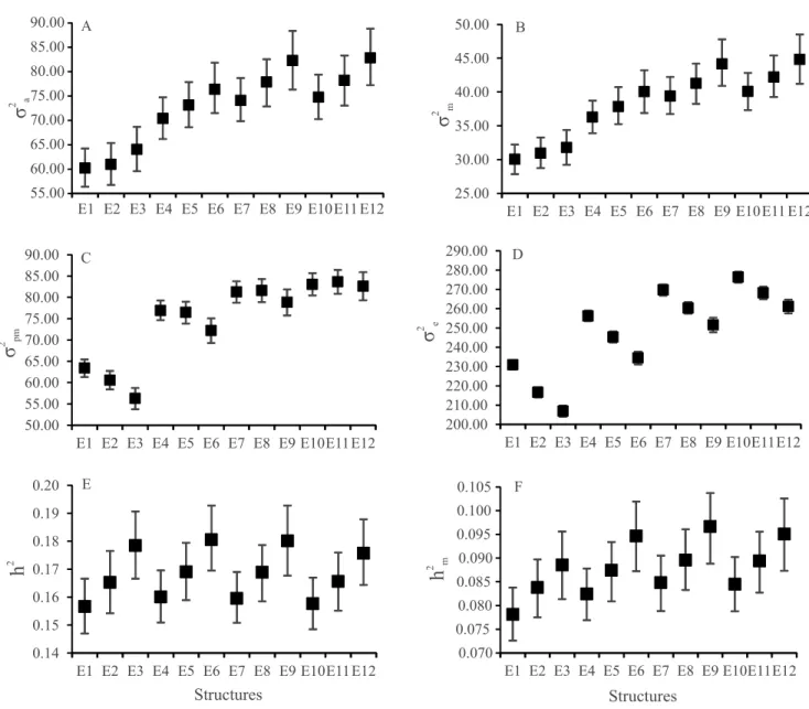
each tested SD for direct (Figure 1 A) and maternal (Figure 1 B) genetic variances. Higher values of direct additive genetic variances were observed for the data sets with higher SD (Figure 1 A). Higher direct and maternal additive genetic variances were found in the E9 and E12 data sets (Figure 1 A and B).
There was also no statistical difference between data sets for 2.5, 3.0, and 3.5 SDs regarding the maternal permanent environmental variance (Figure 1 C). However, by using 2.0 SDs, the E3 and E1 data sets were similar to E2, but differed between each other due to the non-overlapping of the CI. In general, the maternal permanent environmental variance increased as the number of SDs increased. Higher values of maternal permanent environmental variances were observed for 3.0 and 3.5 SDs.
The data sets with a lower number of phenotypic records in each CG, i.e., less animals per CG, presented lower residual variance estimates regardless of the SD used (Figure 1 D). When the number of animals in the CG increased from 3 to 7 and from 3 to 15, residual variances were reduced in 6.28 and 10.38% for 2.0 SDs; 4.26 and 8.49% for 2.5 SDs; 3.47 and 6.72% for 3.0 SDs; and 3.0 and 5.51% for 3.5 SDs,
respectively. In addition, a significant increase was
residual variance (206.91±1.4633), whereas E7 had the highest one (276.42±1.4658).
The data sets with at least 15 animals per CG presented higher direct and maternal genetic variances regardless of SD (Figure 1 A and B). However, these data sets also presented lower maternal permanent environmental and residual variances (Figure 1 C
and D). These results may be responsible for the observed trend towards higher heritabilityestimates and genetic gain (Figure 1 E and 2). Furthermore, the data sets with at least 3 animals per CG presented lower direct genetic variance, as well as higher residual variances, with a trend towards lower h2
estimates and genetic gain (Figure 1 E and 2). The
Figure 1. A posteriori means for: A, direct additive genetic variance (σa2
); B, maternal additive genetic variance (σ
m 2);
C, maternal permanent environmental variance (σpm2
); D, residual variance (σe 2
); E, heritability (h2); and F, maternal
heritability (h2
m), with their respective credibility intervals for the different data sets (E1 to E12) evaluated. For each data set,
obtained results show that the values of all variance components were increased as the number of SDs increased (Figure 1 A, B, C, and D). This explains the similar h2 estimates (direct and maternal) and genetic
gain regardless of the number of SDs (Figure 1 E and F, and Figure 2).
The variation in the total number of animals between data sets allowed a redistribution of variances. The data sets with higher SDs (2.5, 3.0, and 3.5) had higher direct and maternal genetic variances, but lower maternal permanent environmental and residual variances. Therefore, the data sets with 2.0 SDs and at least 3 animals per CG would not be recommended for genetic evaluations in this population.
There were no significant statistical differences
based on CI overlapping among or within the different SDs for direct (h2) and maternal heritability
(h2
m) estimates (Figure 1 E and F). Higher h2 values
(Figure 1 E) were observed for E3, E6, E9, and E12 due to the combination of the greater direct genetic and residual variances (Figure 1 A and D). This shows that, by using at least 15 animals per CG in
genetic evaluations, a higher genetic gain is expected (Figure 2).
Yooko et al. (2010) found h2 equal to 0.22 when
using a CG with at least 8 animals and 3.0 SDs, whereas Silva et al. (2013) reported h2 equal to 0.13
adopting a CG with at least 9 animals. These and the estimates obtained in the present work are lower than those of 0.23–0.61 observed in other studies, which considered different criteria for outlier removal: minimum of 5 animals per CG (Boligon et al., 2008); minimum of 4 animals per CG and 3.0 SDs (Boligon et al., 2009); minimum of 4 animals per CG
(Laureano et al., 2011); and minimum of 3 animals per CG (Lopes et al., 2013).
Faria et al. (2011) obtained higher h2 (0.33) and h2 m
(0.26) estimates than those of the present study by removing the CGs with at least 4 animals. Higher h2
(0.21) and h2
m (0.27) estimates were also found by
Matos et al. (2013), using 3.0 SDs for outlier removal and a CG with at least 7 animals. As in the present study, these works were also conducted via Bayesian inference.
E1 E2 E3 E4 E5 E6 E7 E8 E9 E10 E11 E12
0.00 0.50 1.00 1.50 2.00 2.50 3.00 3.50 4.00 4.50 5.00 5.50 6.00 6.50
Genetic gain (kg)
ΔG Top 1_20 ΔG Top 5_40
Figure 2. Genetic gain (ΔG) of the evaluated data sets (E1 to E12) for 1% of the best bulls and 20% of the best cows (Top
Similar h2
m estimates were reported by Boligon et
al. (2010), who assumed 3.0 SDs for outlier removal
and a minimum of 4 animals per CG; and by Laureano et al. (2011) and Lopes et al. (2013), who used a CG
with at least 3 animals. Silva et al. (2013) adopted at least 9 animals per CG and found maternal heritability estimates lower (0.03) than those observed in all the data sets evaluated in the present study.
It should be highlighted that, even if outlier removal and CG formation are standardized for all genetic evaluation in beef cattle, there would still be differences in genetic parameter estimates due
to the specific features inherent to each population
and to the environmental conditions that animals are subjected to. Therefore, genetic parameter estimates with greater accuracy are expected in genetic evaluations when appropriate criteria are used and
the specific characteristics of each population are
taken into account.
For each SD, the CGs with at least 3 and 7 animals had the highest percentages of common animals, with values of 78.93 and 81.72% for Top 1_20 and Top 5_40, respectively. The lowest percentages were observed between the CGs with at least 3 and 15 animals, with values of 58.47 and 61.47% for Top 1_20 and Top 5_40, respectively. In addition,
higher percentages of common animals were verified
by using 3.0 and 3.5 SDs (Table 2).
Evaluating the number of common animals in different data sets enabled understanding the effects
of outlier removal. It also showed that the empirical outlier removal by using different SD values and a minimum number of animals per CG may affect individual genetic merit and, consequently, the selection process.
Higher genetic gain was observed for the CGs with at least 15 animals associated with 2.5, 3.0, or 3.5 SDs, i.e., for E6, E9, and E12, respectively (Figure 2). However, when these data sets were compared with E1, with a lower genetic gain, these differences were, on average, of 1.06 and 0.77 kg for Top 1_20 and Top 5_40, respectively. When the E6, E9, and E12 data sets were compared with E3, with a lower genetic gain, the differences were, on average, of 0.54 and 0.28 kg greater for Top 1_20 and Top 5_40, respectively.
Limitations on the number of animals per CG
tended to affect genetic gain. The data sets with at least 15 animals per CG showed a trend towards higher genetic gain, whereas those with at least 3 animals, a trend gain towards lower genetic gain. Therefore, the data sets with at least 15 animals per CG may be recommended for genetic evaluations
of this population. This may be justified by the
concept of population sampling; i.e., the higher the number of phenotypic records in each CG, the higher is the chance of this random sampling being close to the average of the population. This way, the representativeness of the genetic parameters will be higher for this population (Cobuci et al., 2006).
Table 2. Percentage of common animals between data sets (E1 to E12) for 1% of the best bulls and 20% of the best cows (Top 1_20) above the diagonal, and 5% of the best bulls and 40% of the best cows (Top 5_40) below the diagonal.
Data set(1) Data set
E1 E2 E3 E4 E5 E6 E7 E8 E9 E10 E11 E12
E1 (2.0–3) 100.00 77.90 57.24 88.46 73.80 55.55 86.55 72.70 54.95 85.91 72.19 54.84 E2 (2.0–7) 81.21 100.00 67.80 73.66 87.22 64.88 72.42 84.99 63.78 71.95 84.15 63.40 E3 (2.0–15) 60.69 70.70 100.00 55.03 64.10 86.17 54.42 63.07 83.65 54.27 62.74 82.55 E4 (2.5–3) 91.82 78.00 58.91 100.00 78.92 58.43 92.96 77.51 57.75 92.09 77.04 57.63 E5 (2.5–7) 78.09 90.99 68.02 81.32 100.00 68.43 77.40 92.41 67.30 76.87 91.35 66.83 E6 (2.5–15) 59.44 68.64 90.21 61.38 71.13 100.00 57.70 67.14 91.57 57.45 66.85 89.85 E7 (3.0–3) 90.45 77.04 58.44 95.04 80.67 60.83 100.00 79.36 58.92 94.86 78.95 58.83 E8 (3.0–7) 77.29 89.41 67.18 80.80 94.55 70.20 82.14 100.00 68.76 78.84 94.46 68.43 E9 (3.0–15) 59.04 67.87 88.40 60.95 70.36 94.05 61.80 71.38 100.00 58.72 68.49 93.85 E10 (3.5–3) 90.07 76.73 58.24 94.38 80.22 60.60 96.38 81.65 61.55 100.00 79.55 59.28 E11 (3.5–7) 77.03 88.89 66.92 80.57 93.91 69.88 81.95 96.09 71.09 82.22 100.00 69.16 E12 (3.5–15) 59.00 67.70 87.61 60.90 70.09 92.95 61.77 71.20 95.66 62.03 71.65 100.00
(1)For each data set, the criteria considered, in between parentheses, were: standard deviations around the mean for outlier removal and minimum number
Conclusions
1. The correct formation of contemporary groups (CGs) of Nellore cattle results in more consistent data sets, which allows obtaining more reliable genetic parameter estimates.
2. The best selection responses are obtained by using 2.5, 3.0, and 3.5 standard deviations and at least 15 animals per CG as criteria for outlier removal.
Acknowledgments
To Associação Brasileira dos Criadores de Zebu (ABCZ), for providing the data for the research; to
Conselho Nacional de Desenvolvimento Científico
e Tecnológico (CNPq), to Coordenação de Aperfeiçoamento de Pessoal de Nível Superior (Capes), and to Fundação de Amparo à Pesquisa do Estado
de Minas Gerais (Fapemig), for financial support; and to the laboratory of biometrics and the scientific
and technological development support division (DCT) of Universidade Federal de Viçosa (UFV), for providing the computers for data analyses and the Cluster equipment for high-performance processing, respectively.
References
AMBROSINI, D.P.; CARNEIRO, P.L.S.; BRACCINI NETO, J.; MARTINS FILHO, R.; AMARAL, R. dos S.; CARDOSO, F.F.; MALHADO, C.H.M. Reaction norms models in the adjusted
weight at 550 days of age for Polled Nellore cattle in Northeast Brazil. Revista Brasileira de Zootecnia, v.43, p.351-357, 2014. DOI: 10.1590/S1516-35982014000700002.
ARAÚJO, C.V. de; BITTENCOURT, T.C.B. dos S.C. de; ARAÚJO,
S.I.; LÔBO, R.B.; BEZERRA, L.A.F. Estudo da heterogeneidade
de variâncias na avaliação genética de bovinos de corte da raça Nelore. Revista Brasileira de Zootecnia, v.40, p.1902-1908, 2011. DOI: 10.1590/S1516-35982011000900009.
ARAÚJO, C.V. de; LÔBO, R.B.; FIGUEREIDO, L.G.G.; MOUSQUER, C.J.; LAUREANO, M.M.M.; BITTENCOURT,
T.C.B. dos S.C. de; ARAÚJO, S.I. Estimates of genetics parameters of growth traits of Nellore cattle in the Midwest region of Brazil. Revista Brasileira de Saúde e Produção Animal, v.15, p.846-853, 2014. DOI: 10.1590/S1519-99402014000400006.
BIGNARDI, A.B.; GORDO, D.G.M.; ALBUQUERQUE, L.G.;
SESANA, J.C. Parâmetros genéticos de escore visual do umbigo em bovinos da raça Nelore. Arquivo Brasileiro de Medicina Veterinária e Zootecnia, v.63, p.941-947, 2011. DOI: 10.1590/ S0102-09352011000400020.
BOLIGON, A.A.; ALBUQUERQUE, L.G. de; MERCADANTE, M.E.Z.; LÔBO, R.B. Herdabilidades e correlações entre pesos do
nascimento à idade adulta em rebanhos da raça Nelore. Revista
Brasileira de Zootecnia, v.38, p.2320-2326, 2009. DOI: 10.1590/ S1516-35982009001200005.
BOLIGON, A.A.; ALBUQUERQUE, L.G. de; RORATO, P.R.N. Associações genéticas entre pesos e características reprodutivas
em rebanhos da raça Nelore. Revista Brasileira de Zootecnia, v.37, p.596-601, 2008. DOI: 10.1590/S1516-35982008000400002.
BOLIGON, A.A.; SILVA, J.A.V.; SESANA, R.C.; SESANA, J.C.; JUNQUEIRA, J.B.; ALBUQUERQUE, L.G. Estimation
of genetic parameters for body weights, scrotal circumference, and testicular volume measured at different ages in Nellore cattle. Journal of Animal Science, v.88, p.1215-1219, 2010. DOI: 10.2527/jas.2008-1719.
COBUCI, J.A.; ABREU, U.G.P. de; TORRES, R. de A. Formação de grupos de contemporâneos em bovinos de corte. Corumbá, MS: Embrapa Pantanal, 2006. 27p. (Embrapa Pantanal. Documentos, 87). Available at: <https://www.embrapa.br/ pantanal/busca-de-publicacoes/-/publicacao/783805/formacao-de-grupos-contemporaneos-em-bovinos-de-corte#>. Accessed on: Feb. 10 2015.
FARIA, C.U. de; TERRA, J.P.; YOOKO, M.J.I.; MAGNABOSCO,
C.U.; ALBUQUERQUE, L.G. de; LÔBO, R.B. Interação genótipo-ambiente na análise genética do peso ao desmame de bovinos
Nelore sob enfoque bayesiano. Acta Scientiarum. Animal Science, v.33, p.213-218, 2011. DOI: 10.4025/actascianimsci. v33i2.8469.
FERRIANI, L.; ALBUQUERQUE, L.G.; BALDI, F.S.B.; VENTURINI, G.C.; BIGNARDI, A.B.; SILVA, J.A. II V.; CHUD, T.C.S.; MUNARI, D.P.; OLIVEIRA, J.A. Parâmetros genéticos
de características de carcaça e de crescimento de bovinos da raça Nelore. Archivos de Zootecnia, v.62, p.123-129, 2013. DOI: 10.4321/S0004-05922013000100013.
GEWEKE, J. Evaluating the accuracy of sampling-based approaches to the calculation of posterior moments. In: BERNARDO, J. M.; BERGER, J.; DAWID, A. P.; SMITH, J. F. M. (Ed.). Bayesian statistics 4. New York: Oxford University, 1992. p. 169-193.
LAUREANO, M.M.M.; BOLIGON, A.A.; COSTA, R.B.; FORNI, S.; SEVERO, J.L.P.; ALBUQUERQUE, L.G. Estimativas de
herdabilidade e tendências genéticas para as características de crescimento e reprodutivas em bovinos da raça Nelore. Arquivo Brasileiro de Medicina Veterinária e Zootecnia, v.63, p.143-152, 2011. DOI: 10.1590/S0102-09352011000100022.
LOPES, F.B.; MAGNABOSCO, C.U.; PAULINI, F.; SILVA, M.C. da; MIYAGI, E.S.; LÔBO, R.B. Genetic analysis of growth
traits in Polled Nellore cattle raised on pasture in tropical region using Bayesian approaches. PLoS ONE, v.8, e75423, 2013. DOI: 10.1371/journal.pone.0075423.
MALLINCKRODT, C.H.; GOLDEN, B.L.; BOURDON, R.M.
The effect of selective reporting on estimates of weaning weight parameters in beef cattle. Journal of Animal Science, v.73, p.1264-1270, 1995. DOI: 10.2527/1995.7351264x.
MATOS, A. de S.; SENA, J. do S. da S.; MARCONDES, C.R.;
BEZERRA, L.A.F.; LÔBO, R.B.; RORATO, P.R.N.; CUCCO,
D. de C.; ARAÚJO, R.O. de. Interação genótipo-ambiente em
Saúde e Produção Animal, v.14, p.599-608, 2013. DOI: 10.1590/ S1519-99402013000300008.
MISZTAL, I.; TSURUTA, S.; LOURENCO, D.; AGUILAR, I.;
LEGARRA, A.; VITEZICA, Z. Manual for BLUPF90 family
of programs. Athens: University of Georgia, 2014. Available at: <http://nce.ads.u-ga.edu/wiki/doku.php?id=application_ programs>. Accessed on: Mar. 3 2015.
PEDROSA, V.B.; ELER, J.P.; FERRAZ, J.B.S.; SILVA, J.A. II de V.; RIBEIRO, S.; SILVA, M.R.; PINTO, L.F.B. Parâmetros
genéticos do peso adulto e características de desenvolvimento ponderal na raça Nelore. Revista Brasileira de Saúde e Produção Animal, v.11, p.104-113, 2010.
ROSO, V.M.; SCHENKEL, F.S.; MILLER, S.P. Degree of
connectedness among groups of centrally tested beef bulls. Canadian Journal of Animal Science, v.84, p.37-47, 2004. DOI: 10.4141/A02-094.
SANTOS, N.P. da S.; FIGUEIREDO FILHO, L.A.S.; SARMENTO, J.L.R.; MARTINS FILHO, R.; BIAGIOTTI, D.;
REGO NETO, A.A. Estimação de parâmetros genéticos de pesos em diferentes idades de bovinos da raça Nelore criados no Meio-Norte do Brasil usando amostragem de Gibbs. Acta Tecnológica, v.7, p.1-7, 2012.
SHIOTSUKI, L.; CARDOSO, F.F.; SILVA, J.A. II V.; ROSA, G.J.M.; ALBUQUERQUE, L.G. Evaluation of an average
numerator relationship matrix model and a Bayesian hierarchical model for growth traits in Nellore cattle with uncertain paternity. Livestock Science, v.144, p.89-95, 2012. DOI: 10.1016/j. livsci.2011.11.002.
SILVA, R.M. da; SOUZA, J.C. de; SILVA, L.O.C. da; SILVEIRA, M.V. da; FREITAS, J.A. de; MARÇAL, M.F. Parâmetros e tendências genéticas para pesos de várias idades em bovinos
Nelore. Revista Brasileira de Saúde e Produção Animal, v.14, p.21-28, 2013. DOI: 10.1590/S1519-99402013000100003.
SORENSEN, D.; GIANOLA, D. Likelihood, Bayesian, and
MCMC methods in quantitative genetics. 2nd ed. New York:
Springer, 2002. 740p.
THE R FOUNDATION. The R Project forstatistical computing. Vienna: The R Foundation, 2011. Available at: <http://www.R-project.org/>. Accessed on: Mar. 5 2015.
YOOKO, M.J.; LOBO, R.B.; ARAUJO, F.R.C.; BEZERRA, L.A.F.; SAINZ, R.D.; ABULQUERQUE, L.G. Genetic associations
between carcass traits measured by real-time ultrasound and scrotal circumference and growth traits in Nelore cattle. Journal of Animal Science, v.88, p.52-58, 2010. DOI: 10.2527/jas.2008-1028.