Optimal Robust Nonlinear LQG/LTR Control with Application to Longitudinal Flight Control

Optimal Robust Nonlinear LQG/LTR Control with application to

Longitudinal Flight Control

Tiago Nunes Sanches;tiago_sanches@sapo.pt University of Beira Interior

Kouamana Bousson - k1bousson@yahoo.com Universidade da Beira Interior

Abstract

As part of the development of a new 4D Autopilot System for Unmanned Aerial Aircrafts (UAVs), i.e. a time-dependent robust trajectory generation and control algorithm, this work addresses the problem of optimal path finding based on the aircraft’s own sensors data output, that may be unreliable due to noise on data acquisition and/or transmission under certain circumstances. Although several filtering methods, such as the Kalman-Bucy Filter or the LQG/LTR, are available, the utter complexity of the new control system, together with the robustness and reliability required of such a system on an UAV for airworthiness certifiable autonomous flight, required the development of a proper robust filter for a nonlinear system, as a way of further mitigate errors propagation to the control system and improve its performance. As such, a new nonlinear LQG/LTR algorithm, validated through computational simulation testing, is proposed on this paper. This research work was conducted in the Laboratory of Avionics and Control of the Department of Aerospace Sciences (DCA) at the Faculty of Engineering of the University of Beira Interior and supported by the Aeronautics and Astronautics Research Group (AeroG) of the Associated Laboratory for Energy, Transports and Aeronautics (LAETA). The author would like to thank Professor K. Bousson for valuable discussions during this work.

Keywords

Optimal Robust Nonlinear LQG/LTR Control with

application to Longitudinal Flight Control

Introduction

Due to the complexity and rhythm of the nowadays life in this modern age, time is becoming increasingly scarce in order to keep up the pace with all the demands. And though, advancements in automation procedures and systems had largely helped to reduce workload and improve schedules, there is still an important gap that must be fulfilled. For instance, whilst actual flight plan fulfilment requires 4D navigation, existing autonomous navigation procedures are mostly done in 3D because of the stringent certification requirements for 4D flight and due to the complexity in coping with time of arrival at waypoints. Therefore, there is a need for the development and testing of an algorithm that, when implemented on an aircraft’s autopilot system, will enable the aircraft to autonomously fulfil its scheduled time-of-arrival at a designated waypoint. As an initial step on that development process, the present work focuses on the simulated testing of improved and up-to-date optimal control and filtering methodologies that will be implemented in the aforementioned algorithm. More precisely it presents the background theory and simulated results of an LQG/LTR controller method when applied to a Classical Atmospheric Disturbances Simulation Test of an UAV on stable levelled flight.

1. Theoretical Background

In order to achieve the desired level of flight efficiency and safety, especially with beyond visual range UAVs flights, it is crucial to ensure proper control of the aircraft through error mitigation and pilot/operator’s workload reduction technologies. This level of precision flight control is achieved by resorting to the physical implementation of computerized systems that allow for automated flight. These systems are generally known as Autopilot Systems, and they combine the information provided by the aircraft’s onboard sensors with the known Flight Dynamics Equations, Aircraft’s Data, to correlate them through an algorithm and achieve a timely Optimal Control solution that will be commanded by the system to the Aircraft’s Control Surfaces and Engine(s). This algorithm is referred to as an Optimal Control Method. Following on from previously developed work [1] and tests results, this work focuses on the further improvement of the LQR Controller Method by addressing the treatment of the unavoidable noise on data acquisition sensors with the implementation of a Kalman Filter upon the LQR, a combination usually referred to as a LQG Controller Method. The theoretical background for such methods is provided on the following sub-sections.

1.1. LQR Controller Method

In a LQR controller, the time-continuous linear system, referring to longitudinal control, is described by [1][2][3][4]:

x AxBu ,

_x

IR

n _and

_u

_

_IR

m ₍₁₎

The cost function is defined as:

 

0 ,

J

_

F x u dt (2)

Where: x– Aircraft’s Longitudinal State variation; A– Jacobian Matrix concerning the State

Vector; x– State Vector; B– Jacobian Matrix concerning the Control Vector; u– Control Vector;

J– Cost Function; F– Function of the state and control vectors.

As for longitudinal flight, A is the Jacobian matrix of F concerning the aircraft’s state vector

x and Bthe Jacobian matrix concerning the aircraft’s control vector u obtained from linearization.









































































0 0 0 0 0 0 0 0 0 0 0 0 0 0 0 0 ____ _ , , , , ; , , , , ; T T x V u V T T x u T T x q u q T T x u T T e T f x u f x u f x u f x u A B f x u f x u f x u f x u x V q u          _   _       _   _      _{ } _{ }                       (4)

Where u must be such that it minimizes the coast function on the following way:

   

₀





: : T T

u u x J u 

_

 x Qx u Ru dt (5)

The feedback control law that minimizes the cost function in (eq. 3) is described by:

u  K x (6)

Where _K m n _{is the system’s gain matrix determined by:} 1 T

K R B P  (7)

This cost function (eq. 2) is often defined as a sum of the deviations of key measurements from their desired values. However, the main problem while properly scaling a LQR controller, i.e. fine-tuning the controller for optimal performance, resides in finding the adequate weighting factor’s Q and R matrices. In general LQR design, Q and R are simply determined by Bryson’s method [1][5], where each state (Q matrix) and control (R matrix) parameter (diagonal element) is calculated in relation to its maximum amplitude:

2 2 ,max ,max ___ 1 1 _ ii ii i i Q R x u   (8)

Where: A– State Vector Jacobian Matrix;

x

0– Initial State Vector;

u

0– Initial Control Vector; B

– Control Vector Jacobian Matrix; V – Aircraft’s Speed;  – Path Angle; q– Pitch Rate; – Pitch

Angle;



e– Elevator Deflection;



T– Throttle Setting; u– Control Vector; x– State Vector; J–

Cost Function;

Q

– State Vector Weighting Matrix; R– Control Vector Weighting Matrix; K–

System’s Gain; P– P Problem.

Although this method being a good starting point for trial-and-error iterations on the search for the intended controller results, it is somehow limited by its maximum state values as, even though the control values are limited only by their control surface’s maximum physical properties, they lack a more proper optimization algorithm.

However, a better alternative method, proposed by Jia Luo and C. Edward Lan [6], is available, since 1995, for the Q and R matrices estimation. The R matrix is still determined using Bryson’s method (eq. 8) [1][5], as the problem lies, as noted before, in the determination of the optimal state values of the Q matrix. In this method, the cost function J (eq. 2) is minimized by a Hamiltonian matrix H, which is used to determine P.Q and R are, as stated before, weighting matrices for, respectively, the state and control variables, and must be respectively defined as positive-semidefinite and positive-definite. Considering the Theorem whereby a symmetrical matrix has only real eigenvalues, it can be deduced that when _QQT,_{Q , all its eigenvalues} 0 are



i

 

Q 0and, when R R R T, 0, then all its eigenvalues are



i

 

R 0. The R matrix is

therefore a Penalization (or Ponderation) matrix of the control vector, which allows for some flexibility upon its generation, and is therefore calculated by Bryson’s method (eq. 8). However, the Q matrix must be such that its eigenvalues match the eigenvalues from a group I Hamiltonian matrix H. Accordingly to the principle of the Pontriagin’s Maximum, the Hamiltonian matrix is associated to the LQR’s “P Problem” (eq. 9)[1]. This consists in the calculus of the H matrix by minimizing the control’s output cost function (eq. 6) while restricted by the LQR’s longitudinal time-continuous linear equation x (eq. 1).

 





1 0 T T T T x Ax Bu _{A BR B} P H Q A J u x Qx u Ru dt      _{  }  _{ }  _{ } _{ }    



(9)

The eigenvalues of H are thereby symmetrically distributed in relation to the imaginary axis, thus having positive and negative symmetrical real parts only. And as the “P Problem” is part of the  matrix of the LQR’s feedback system described as follows [1]:

1 T

 A BR B P   (10)

P is found by solving the continuous time algebraic Riccati’s equation [2][7], in (eq. 11):

1 ₀

T T

A P PA PBR B P Q_{ }  _{  (11)}

As the eigenvalues of  are the same of those of the Group I of the Hamiltonian matrix H, they can be specified as [1]: 1 1 1; ; n n n i i             _{ }  (12) With Re

 



n 



n 0;Im

 



n 



n 0 .

Therefore, the state matrix Q must be determined such that [1]:





: det i 0

i



I H

   (13)

Where I is an Identity matrix. For simplified calculations, it is enough to use the state matrix A’s eigenvalues, but in order to minimize the cost function J (eq. 2) under certain imposed flight qualities, and therefore, these eigenvalues must be subjected to such impositions. The Q matrix is thereby defined as a diagonal matrix composed by a single vector qi =



q q1 2 qn



T

. To satisfy the prior condition (eq. 13), qi must be such that [1]:

 



 



in order

 



 



2 to minimize 1 : i i det i i 0 n i i i i f q



I H q J q f q       



(14)

Finding theqivalues that satisfy ( )J q will give the solution to Q. However, in order to ensure

that Q comes as a positive-semidefinite matrix with Group I eigenvalues, the “diagonal vector” is rather defined by the square root of its elements, i.e. 2 2 2

1 2

T

i n

q _{ }q q q _ , which prevents Q from having undesired negative values in its diagonal [1]. A new control law comes as:





ref ref

u u K x x (15)

This allows the LQR controller to fully stabilize an aircraft state and control variables for optimized R and Q weighting matrices as the control output vector is given in function of the deviation from the required output (

u

ref) to maintain the aircraft on the desired attitude

described by the reference state vector

x

ref[1].

1.2. Kalman-Bucy Filter

From the general discrete-time domain Kalman Filter theory, the estimator is given by:



 



ˆ ˆ ˆ ˆ

x Ax L y Cx    A LC x Ly 

(16)

The Kalman filter is applied whenever the uncertainties (or noise present either in the model, in the observations or in both) are not negligible and therefore, cannot be ignored. This means that





0

and





0

.These two random vectors are assumed to be white noises with Gaussian distribution [8], i.e. both have null averages and each one has over-time uncorrelated values.

 

 

X AX t Y Cx t           (17)

The Kalman filter’s equation (in time-continuous domain, i.e. Kalman-Bucy Filter) follows the same logic reasoning as for the discrete-time domain, but with two particular details [8]:

 







* * 1 0 0 0 ˆ0 0 ˆ0 T P AP PA PC R CP Q P t P E x x x x         _{     }  _{ }  (18)

Where

ˆx

₀ is the assumed initial state for the system considered for the solving of the differential equation (eq.16).

2. The weighting matrices are given by [8]:

 

T

 

T

Q E



and R E



(19)

Using the above equations (eq.18) and (eq.19), enables the achievement of the solution

P t

 

_k for the differential matricial equation of Riccati on the instant

t

_k, being that [8]:

 

,



:



P t _{  }



t  t_t ₍₂₀₎

means that the estimative is very accurate [8].

Be it

P

_k



P t

 

_k the solution of the Riccati’s equation on the instant

t

_k, the gain is given by [8]:

 

1

k k k

L t _L _P CR ₍₂₁₎

The state filtering estimation equation is thereby as follows [8]:

ˆ ˆ ( )( ˆ)

x Ax L t y Cx   (22)

Wherein,

x

ˆ

_k₁ must be calculated as the solution of the differential equation (eq.22) [8].

1.3. LQG Controller Method

In control theory, the LQG, or Linear Quadratic Gaussian control problem, is one of the most fundamental problems on optimal control. Essentially, the LQG controller is a Kalman Filter, i.e. a Liner Quadratic Estimator, applied to a LQR, i.e. Linear Quadratic Regulator and deals with uncertain linear systems disturbed by additive white Gaussian noise, while having incomplete state vector information (i.e. not all the state vector variables are measured and and/or readily available for feedback, meaning they are unknown variables) and undergoing control subject to quadratic costs. “Moreover, the solution is unique and constitutes a linear dynamic feedback control law that is easily computed and implemented. Furthermore, it is also fundamental to the optimal control of perturbed non-linear systems.” [10][11]

“The separation principle guarantees that both the LQE and LQR can be designed and computed independently. LQG control applies to both linear invariant systems as well as linear time-varying systems. The application to linear time-invariant systems is well known. The application to linear time-varying systems enables the design of linear feedback controllers for non-linear uncertain systems.” [10]

1.3.1. Continuous-Time Linear System LQG

Since the LQR requires a linearization of the system in order to be implemented, the same linearized system can be used for our advantage as it enables the use of the easier to implement linear LQG for a continuous-time system, instead of the non-linear option.

Given the following time-continuous linear dynamic system [10][11]:

( ) ( ) ( ) ( ) ( ) ( ) ( ) ( ) ( ) ( ) x t A t x t B t u t t y t C t x t t





     _{ }  (23)

Where:x is the state vector;

x

is the estimation of the state vector x;u is the control inputs vector;

y

is the vector of the measured outputs available for feedback;



( )

t

is the additive white Gaussian noise that affects the system;



( )

t

is the measurement of the white Gaussian noise. The objective is to find the control input history

u t

( )

which at every time

t

may depend only on the past measurements

y t

 



,0

 

t



t

such that the following cost function is minimized [10][11]:

0

( ) ( ) T ( ) ( ) ( ) ( ) ( ) ( ) , 0, ( ) 0, ( ) 0

T T T

JE x T Fx T_ 



x t Q t x t u t R t u t dt F_  Q t  R t  (24)

“Where

E

denotes the expected value. The final time (horizon)

T

may be either finite or infinite. If the time horizon tends to infinity, the first term

_{x T Fx T}

T

( ) ( )

_{of the cost function}

becomes negligible and irrelevant to the problem. Also, to keep the costs finite, the cost function has to be taken to be

J T

/

” [10].

The LQG controller that solves the LQG control problem is specified by the following equations [10][11]:









ˆ( ) ( ) ( )ˆ ( ) ( ) ( ) ( ) ( ) ( ) , (0)ˆ ˆ (0) ˆ ( ) ( ) ( ) x t A t x t B t u t K t y t C t x t x E x u t L t x t            (25)

“The matrix

K t

( )

is called the Kalman gain of the associated Kalman filter represented by the first equation. At each time

t

this filter generates estimates

x t

ˆ( )

of the state

x t

( )

using the past measurements and inputs” [10].The Kalman gain

K t

( )

is computed from the matrices

( )

A t

and

C t

( )

, as well as the two intensity

V t

( )

and

W t

( )

associated with the white Gaussian noises



( )

t

and



( )

t

and finally

_{E x}

_

(0) (0)

_x

T

_





”. These five matrices determine

the Kalman gain through the following associated matrix Riccati differential equation [10][11]:

1 ( ) ( ) ( ) ( ) ( ) ( ) ( ) ( ) ( ) ( ) ( ) (0) (0) (0) T T T P t A t P t P t A t P t C t W t C t P t V t P E x x         _{  }     (26)

Given the solution

P t

( ),0

 

t T

, the Kalman gain equals to [10][11]: 1

( ) ( ) T( ) ( )

K t _P t C t W t ₍₂₇₎

The matrix

L t

( )

is called the feedback gain matrix and is determined by the matrices

A t

( )

,

( )

B t

,

Q t

( )

,

R t

( )

and

F

through the following associated matrix Riccati differential equation [10][11]: 1 ( ) ( ) ( ) ( ) ( ) ( ) ( ) ( ) ( ) ( ) ( ) ( ) T T S t A t S t S t A t S t B t R t B t S t Q t S T F          (28)

Given the solution S t( ),0 t T the feedback gain equals to [10][11]: 1

( ) ( ) T( ) ( )

L t R t B t S t (29)

While the first of the two Riccati matrices is running forward in time, the second one is running backwards in time. This similarity in between the two Riccati matrices is known as duality. The first matrix Ricatti differential equation solves the linear-quadratic-estimation problem (LQE), while the second matrix Riccati differential equation solves the linear-quadratic-regulator problem (LQR). These problems are dual and together solve the linear-quadratic-Gaussian problem (LQG).

“When

A t

( )

,

B t

( )

,

C t

( )

,

Q t

( )

,

R t

( )

, and noise intensity matrices

V t

( )

and

W t

( )

do not depend on

t

and when

T

tends to infinity, the LQG controller becomes a time-invariant dynamic system, meaning that both matrix Ricatti differential equations may be replaced by the two associated algebraic Riccati equations” [10].

1.4. LQG/LTR Controller Method

The Loop Transfer Recovery, or LTR for short, was specifically developed to overcome robustness problems in the LQG control method, hence it is most commonly known as the LQG/LTR Method, which stands for Linear Quadratic Gaussian Control synthesis with Loop Transfer Recovery [12]. It was firstly introduced by Doyle and Stein in [12]. “The point of this approach is based on the fact that using the observer has no effect on the closed loop transfer function but has a harmful influence on the robustness properties. The LQG/LTR method aims at modifying the Kalman filter so that the harmful effects on stability margins are attenuated by making the open loop transfer function of the system (usually referred to as plant) with observer asymptotically approximate the one which this would without the observer included”

[13]. In fact, and accordingly with Chen, the LQG alone is “not an optimal control design method” [14], “not even a stochastic control design method” [15], and “uses Fictitious KF” [14](Kalman Filter). Therefore, “LQG/LTR should be regarded as one word” [14], as it constitutes “a robust control design method that uses LQG control structure” [15]. So, be it

( )

G s a linear continuous-time plant with state-space matrices A B C, , , and

D



0

. From the system’s model [16]: (y C ) x Ax Bu H x y Cx Du       _{ }  (30)

Where x, u and

y

are respectively the system’s state vector, the algorithm’s calculated control

vector, and the system’s outcome of that control input.

x

is the system’s state variation from the initial state, x, in time due to the control vector input, u and the respective measured

system’s outcome, i.e. the system’s state reaction to that input,

y

. The estimator, ˆx, is the system’s state estimation based on the previous system’s outcome,

y

. And the system’s feedback of the difference in between its known, measured current state,

y

, and it’s prior estimative, ˆx, is given by the estimation’s variation parameter, ˆx, as [16]:

ˆ ˆ ( ˆ) ˆ x Ax Bu H y Cx u Gx Gx             (31)

The LTR can be applied either at the entrance of plant, in which case

G

is constant and H is

variable, or at the exit of the plant, in which case

G

is variable and H is time invariable

(constant). The goal is then to minimize the cost function [16]:

0

min_J _{y t y t}T( ) ( )_{u t Ru t dt}T( ) ( )_

 



(32)

Considering _{Q C C} T _and

_R





_I

_with

 

₀

_{. Through Ackermann’s Formula [16], Q Q} T ₀

and hence _{R R} T _0_{. Then, in accordance with the LTR fundamental Theorem, if the primal}

state is controllable, the dual state is observable, the Plant’s Nominal Transfer Function Matrix on frequency-domain,G sN( ), is a square matrix, and its zeros/poles are on LHP (Left-Half Plan)

[16]:

1 T

G_B P ₍₃₃₎

Where _{P P} T _0 _{is the solution to the Algebric Riccati’s Equation given by [16]:} 1 0 T T T PA A P C QC PBB P



     (34)

And so, conerting the above to an equivalent feedback controller in the transfer-function form the LQG/LTR gain, K, is given by [16][17]:





₁ 1





₁



 



0

lim ( )K s C I A B C I A H, with det I A BG .det I A HC 0

    



 

          (35)

2. Nonlinear System LQG/LTR Controller Method Solution

However, as good as an advantageous approach the LQG/LTR method might be, in its current form it is only applicable to linear system’s models (plants). Meanwhile, Aircraft’s Navigation is inherently nonlinear and time-continuous. Therefore, there is a need to adapt the previously described method’s equations and formulation for continuous-time nonlinear LQG/LTR system’s application. For that purpose, the method should comply with two pre-requirements:

|| || 0 ( ) lim 0, ( ) is nonlinear || x || Find Q || ( ) || x that satisfies f x _{f x} f x x   _{ }    _{ }  (36) The system’s model (plant) thereby is defined as:

ˆ ( ) , with 0 x Ax Bu f x Du y Cx Du       _{ }  (37)

The linear LQG/LTR system’s model is given by the previous (eq.30)[16]:

 





ˆ ˆ ˆ x Ax Bu f x H y Cx y Cx          (38)

Therefore, it is easy to see that, when replacing

y Cx



on the first equation, we get our nonlinear f x( ) for the estimator [16]:





ˆ ˆ

xAx Bu H Cx Cx   (39)

Interestingly enough, Cx Cx x x ˆ ˆ, which is nothing less than the estimation’s error,

x

[16]:

ˆ

x x x  (40)

Also, the variation in estimation’s error is given by [16]:

x Ax (41)

It would seem from here, that the first criteria for this method is not met as:

|| || 0 || || 0 || || 0

ˆ ˆ

( ) ( ) ( )

lim 0 lim 0 lim 0

|| || || || || || x x x f x H Cx Cx H x x x x x           (42)

Which, as the fraction’s bottom element converges for zero faster than the upper element, would not hold true to the condition meaning that f x

 

would converge for infinty rather than to zero as intended. However, remember that from (eq.40), the estimation’s error,

x

, is null if A is stable [16], meaning that:

 





 

|| || 0 || || 0 || || 0 || || 0 || || 0

ˆ 0 0

lim 0 lim 0 lim 0 lim 0 lim 0 0 0 0

|| || || || || || || || x x x x x f x H x x H x x x x                  (43)

Thereby, the condition holds true for that f x( ), as long as A is stable. This becomes even more

evident the greater the order of the nonlinear system, as e.g.:

 



2





2



2

|| || 0 || || 0 || || 0 || || 0

|| || 0

ˆ 0

lim 0 lim 0 lim 0 lim 0

|| || || || || || || || lim 0 0 0 x x x x x H x Cx Cx H x f x Hx x x x x Hx                    (44) Therefore as long as A is stable, which the LQG ensures (through the linearization of the flight

system’s equations as pre-requirement for LQR implementation), not only the second order of Taylor’s expansion, f x( ), will satisfy the criteria, as, as it would be desirable, it ensures over-time estimation accuracy as

x



0

.

With f x( ) borrowed from the already existing method, only the matrix

Q

remains to be defined in such a way that it meets the established criteria.

From [18], for a multivariable quasilinear stochastic system (Aircraft’s Navigation fits in the description), where

A B

, , and

C

matrices variations, and (noise) variations are null, it is safe to assume

P

  

0

P const

.

 

C B

. Therefore, on Matlab®_{, the command that would give the}

LQR solution lqr(AT_,CT_{,Q,R) is replaced by the modified command lqr(A,B,Q,R) in order to}

achieve the LQG solution. The calculated eigenvalues on previous work, for the longitudinal flight’s short and long period modes, are given by [1]:



 



1,2 SP LP 2, 25 19843i 0,0693 0,1588i









     (45)

The LQR’s weighting matrix

Q

is traditionally calculated by the Bryson’s Method (eq. 8)[1]. Quickly it is perceived that the Bryson’s Method directly satisfies the second criteria, for positive eigenvalues only, as, from LQR (eq.3):

 

_{2 2} ,max ,max T T T T i i x x x f x x Qx x Qx x x x x           (46)

However, on the previous work [1], matrix

Q

was calculated through a new method presented by Jia Luo and C. Edward Lan in 1995 [6], which proved to be a more robust and reliable method. For the Luo and Lan Method,

Q

must be such that:

 



 



 



 



 





 





2 that minimizes 1 2 1 : det 0 0 n i i i i i i i n i i i i f q I H q J q f q x J q f q x                





(47)

This method as the advantage of being able to calculate the

Q

matrix in order to satisfy the mentioned condition despite the use of negative poles/eigenvalues,



. Therefore, this method allows for the continuation from the previously achieved eigenvalues. Using the same eigenvalues will also provide a better comparison term between the results of this Quasilenear LQG/LTR method with the previously achieved results using only LQR.

3. Numerical Simulation

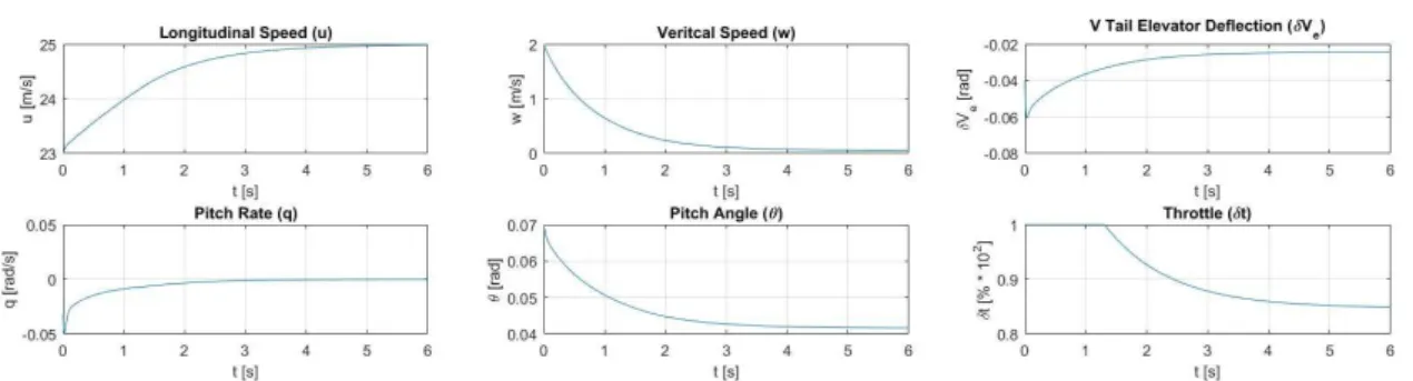
For space saving purposes, only part of the results is showcased in this article. The results obtained for the LQG solution, without LTR, using Aoki’s Method are shown on figure 1, while the results obtained for the LQG/LTR, using Aoki’s Method for the LQG and an adaptation of the Luo and Lan Method for the recalculation of the Q matrix are shown on figure 2.

For better comparison terms, the numerical model follows on the same one used for the LQG vs Batz-Kleinman Classical Disturbances Simulation Test of the previous work [1], for the given state vector

X





25.0000 0.0000 0.0000 0.0416



T, which, upon inflicted a disturbances vector

2

x

, becomes

X

i





23.0000 2.0000 0.0300 0.0716



T, and C is an 8x8 identity matrix.

Figure 1 – Linear Quadratic Gaussian Control Method results on a Classical Disturbances Simulation Test.

Figure 2 – Linear Quadratic Gaussian with Loop Transfer Recover Control Method results on a Classical Disturbances Simulation Test.

As it is easily perceptible from the comparison between the two figures, the new LQG/LTR method offers a much faster convergence to the reference values to the same degree of smoothness as the standalone LQG method and its predecessor in which it is build upon, the LQR method. As this new method simply replaces the calculation formulae for the Q matrix,

and uses the same Matlab® _{lqr command due to the Aoki method, this LQG/LTR with Aoki}

method doesn’t require an increase on computational workload, remaining as nimble as the original non-filtered LQR method. And the diagonal values of the new Q matrix are given by



0.0073 0.0075 0.0156 0.0122 0.0113 0.0006 0.4572 0.0663



T

i

q



.

Conclusion

In conclusion, as both the LQR and the LQG ensure a stable A matrix, the resource to the Luo and Lan Method enables the use of the established LQG/LTR solution formulae for the nonlinear continuous-time domain systems, by simply recalculating the Q matrix values to be used, without having to resource to the separation principle, and separately design a LQR and an Extended Kalman Filter (EKF), which had otherwise proven inadequate as they had lead to several complications with matrix dimensions disagreements in previous attempts. This provides a very quick, easy, and low-computational solution for nonlinear continuous-time systems LQG/LTR method. It is easily seen that the LQG/LTR results converge far faster and smoother than the LQG alone, proving both the LQG/LTR concept and the new method.

References

[1] T. Sanches. Longitudinal Flight Control with a Variable Span Morphing Wing. LAMBERT Academic Publishing, Balti, Moldova, 2017.

[2] B. N. Pamadi. Stability, Dynamics and Control of Airplanes. AIAA, Inc. Hampton, USA, 1998. [3] E. E. Larrabee. Airplane Stability and Control. Cambridge University Press, Cambridge, UK, 2002.

[4] B. Etkin. Dynamics of Flight Stability and Control. John Wiley & Sons, Inc. s.l., 1996. [5] J. B. Moore. Linear Optimal Controler. Prentice-Hall, s.l., 1989.

[6] Luo, J.; Lan, C.E.: 'Determination of Weighting Matrices of a Linear Quadratic Regulator'' Journal of Guidance, Control and Dynamics, Vol. 18 no. 6 (1995), pp. 1462-1463.

[7] R. C. Nelson. Flight Stability and Automatic Control. McGraw-Hill Book Company, New York, USA, 1989.

[8] K. Bousson. Unidade Curricular de Avónica: Teoria dos Observadores e da Filtragem de Kalman-Bucy (No domínio contínuo). FEUBI-DCA, Covilhã, Portugal, 2016.

[9] A. Cerdeira. Miniprojeto de Avionica Parte Pratica – Processamento de Dados Avionicos. UBI, Covilhã, Portugal, 2016

[10] Wikipedia. Linear Quadratic Gaussian Control. https://en.wikipedia.org/wiki/Linear %E2%80%93 quadratic%E2%80%93Gaussian_control (03/07/2017)

[11] Athans, M.: The role and use of the stochastic Linear-Quadratic-Gaussian problem in control system design'' IEEE Transaction on Automatic Control, (1971).

[12] Stein, G.; Athans, M.: "The LQG/LTR Procedure for Multivariable Feedback Control Design'' IEEE Transaction on Automatic Control, vol.AC-32 no. 2 (1984), pp. 105-114.

[13] Kozáková, A.; Hypiusová, M.: ''LQG/LTR based reference tracking for a modular servo'' Journal of Electrical Systems and Information Technology, no. 2 (2015), pp. 347-357.

[14] X. Chen. Advanced Control Systems II (ME233): Key Notes for Discussion 7, 2013.

[15] Lavretsky, E.: ''Adaptive Output Feedback Design Using Asymptotic Proprieties of LQG/LTR Controllers'' IEEE Transaction on Automatic Control, Vol. 57 no. 6 (2012), pp. 1587-1591. [16] A. A. G. Siqueira. SEM 5928 – Sistemas de Controle: Aula 8 – Projeto LQG/LTR, Universidade de São Paulo, Brazil, 2014.

[17] X. Chen. Lecture 9(ME233): LQG/Loop Transfer Recovery (LTR), UC Berkeley, USA,2014. [18] M. Aoki. Optimization of Stochastic Systems, Topics in Discrete-Time Systems. Academic Press, New York, USA, 1967.