A METHODOLOGY TO ASSESS ROBUST STABILITY AND ROBUST
PERFORMANCE OF AUTOMATIC FLIGHT CONTROL SYSTEMS
Alex Sander Ferreira da Silva
∗ [email protected]Henrique Mohallem Paiva
† [email protected]Karl Heinz Kienitz
‡ [email protected]∗Empresa Brasileira de Aeronáutica (EMBRAER) - Sistemas de Comando de Voo
Av. Brigadeiro Faria Lima, 2170 – São José dos Campos, SP – 12227-901 – Brasil Tel: +55 12 3927-0277, Fax: +55 12 3927-4525
†Mectron Engenharia, Indústria e Comércio S/A. - Gerência de Engenharia de Sistemas
Av. Brigadeiro Faria Lima, 1399 – São José dos Campos, SP – 12227-000 – Brasil Tel: +55 12 2139-3500, Fax: +55 12 2139-3535
‡Instituto Tecnológico de Aeronáutica (ITA) - Divisão de Engenharia Eletrônica
Praça Marechal Eduardo Gomes, 50 – São José dos Campos, SP – 12228-900 – Brasil Tel: +55 12 3947-6931, Fax: +55 12 3947-6930
RESUMO
Uma metodologia para avaliar a estabilidade e o desem-penho robustos de sistemas automáticos de comando de voo
Esse artigo apresenta uma metodologia para avaliar a estabi-lidade robusta e o desempenho robusto de sistemas automá-ticos de comando de vôo. A ferramenta matemática utilizada na metodologia proposta é o valor singular estruturado, µ. Para fins de comparação, o artigo utiliza uma metodologia largamente utilizada na indústria aeronáutica para mensurar as características mencionadas. Os problemas dessa meto-dologia são discutidos e é mostrado que o método proposto é uma elegante alternativa para contornar as desvantagens do método industrial. Um procedimento passo a passo é apresentado, incorporando as vantagens da abordagem atu-almente utilizada na indústria e eliminando suas fraquezas.
Artigo submetido em 09/11/2010 (Id.: 01217) Revisado em 29/01/2011, 24/03/2011
Aceito sob recomendação do Editor Associado Prof. Luis Fernando Alves Pereira
PALAVRAS-CHAVE: Controle Robusto, Valor Singular
Estruturado, Realimentação, Sistemas Automáticos de Co-mando de Voo
ABSTRACT
This article presents a methodology to assess the robust sta-bility and the robust performance of automatic flight control systems (AFCS). The mathematical tool used in the proposed methodology is the structured singular value,µ. For compar-ison purposes, the paper uses a method largely employed in the aircraft industry to measure the quoted AFCS attributes. The issues existing in this methodology are discussed and it is shown that the proposed method presents one elegant path to deal with the mentioned drawbacks. A step by step pro-cedure is provided, incorporating the advantages offered by the approach currently used in the industry and eliminating its weaknesses.
KEYWORDS: Robust Control, Structured Singular Value,
1
INTRODUCTION
Modern automatic flight control systems (AFCS) design and analysis is a model-based activity. This means that, in a pre-liminary step, it is necessary to develop aircraft models as well as the models of the aircraft main peripherals, like ac-tuators, engines, etc. Modeling comprises a vast engineer-ing area and its detailed discussion lies beyond the scope of this paper. Fortunately there is an extensive and rich litera-ture presenting the main aspects of aircraft modeling (Cook, 2007; Pamadi, 2004; Phillips, 2004; Roskam, 2003; Roskam and Lan, 2003; Stevens and Lewis, 2003; Yechout and Mor-ris, 2003).
One important output of the modeling activity is the under-standing of the possible inaccuracies that might be present in the particular model under study. This knowledge can be ap-plied during the design phase in order to minimize the possi-bility of AFCS rework during the final flight test phase, since it is well known that major changes during this stage are time consuming and expensive.
Broadly speaking, the robustness assessment consists in ver-ifying if the required performance and stability are main-tained, considering all possible plant variations within their assumed bounds. Such verification does not depend on the particular choice of the AFCS design synthesis technique. In fact, they can even be used as judgment criteria of the quality of a specific AFCS controller.
Since having reliable measures of control law robustness is an unquestionable necessity, flight control laws design-ers keep a constant interest on the subject. A procedure to check AFCS robustness largely used in the aeronautical in-dustry employs the concept of open loop transfer functions (Gangsaas, Blight and Caldeira, 2008; Gangsaas et al., 2008). This article revisits this procedure and points out its limita-tions. The subsequent focus is to show how the concept of structured singular valueµcan be used to fill in the existing gaps. The final goal is to provide a step by step methodology which incorporates the advantages offered by the currently used method and eliminates its weaknesses.
The text is organized as follows. Section 2 presents a general layout, applicable to a broad class of AFCS control laws. It also identifies the AFCS elements responsible for guarantee-ing robustness. Section 3 provides a short description of one particular AFCS. It also presents the aircraft models, valid for one flight condition, as well as the adopted modeling of the flight controls elements. Section 4 discusses a method widely used in the aircraft industry to assess AFCS robust
stability and performance. Section 5 provides the add-ons sufficient to overcome the present limitations of the method from Section 4. The analysis plots provided in Section 4 and 5 are based on the models described in Section 3. Final re-marks are given in Section 6.
2
AFCS GENERAL LAYOUT
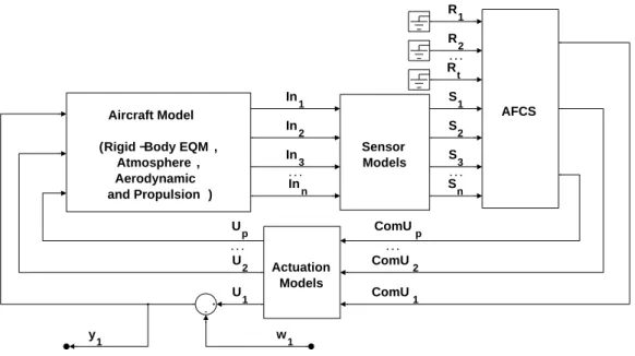
The model arrangement depicted in Fig.1 shows the archi-tecture of a real AFCS application (aircraft, sensors, actua-tors, flight control computer, pilot, etc). Aircraft dynamics is represented by a multiple-input multiple-output (MIMO) system, having as inputsU1,U2, . . . ,Upand as outputs the signals In1,In2,In3, . . . ,Inn. The sensors dynamics are located inside the block Sensor Models.
The AFCS control law uses the measured signals S1, S2,
. . . ,Sn and the reference signalsR1,R2, . . . ,Rt, which are provided either by the pilot or by the navigation computer. The control algorithm provides the demands for the aircraft inputs, ComU1,ComU2, . . . , ComUp. Pure time delays, representing either the data transportation on digital buses or the computer calculation lag, are also implemented inside the block AFCS.
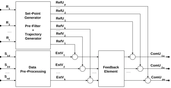
Figure 2 shows a general AFCS layout. The signal pre-processing block computes the signals estimate to be used in the control law. It takes the available measurement from the aircraft sensors and performs data computation and fil-tering. The point generator computes the feedback set-points, based on either the pilot or navigation computer puts. Finally, the feedback section computes the aircraft in-puts demands based on the errors between the estimated vari-ables and the respective set-points.
The sensed signals used by the control algorithm,S1d,S2d, . . . ,Snd, are the delayed version of the sensor outputs. This delay is due to the transport delay inherent to digital buses. The aircraft input demands produced by the control law, ComU1u,ComU2u,. . . , ComUpu, also suffer a delay prior to reaching the actuators.
In 1
In 2
In 3
Inn
S 2
S 3
Sn S
1
ComU 1 ComU
2 U
2
U 1
ComU p U
p
R 1
R 2
R t
. . . . . .
. . .
. . . . . .
Reference Setting
Actuation Models
AFCS
Sensor Models Aircraft Model
(Rigid −Body EQM , Atmosphere , Aerodynamic and Propulsion )
Figure 1: Model Arrangement - Overview
3
SHORT DESCRIPTION OF ONE
SPE-CIFIC AFCS
The AFCS which is presented in this section is an example of aψhold/ψcapture control law. In other words, this is an auto pilot function which holds the desired heading and also allows the proper transitions from one initial heading to the final one.
Another function of this AFCS is the regulation of the side slip angle,β, around zero. This feature is important for two basic reasons: 1 - This is what damps out the aircraft Dutch roll mode. 2 - Compared to a simple regulator ofβ˙ (which comprises the conventional Yaw damper of commercial air-craft), a regulator ofβ provides the same features and also the automatic trimming of the aircraft lateral axis.
The objective is not to present how this final design was achieved. The goal is to provide a design, with performance compatible with a good auto pilot, and then use it to aid in the presentation of the methods described in Sections 4 and 5.
3.1
Aircraft Dynamics
A non-linear model of the Boeing 747 aircraft was assem-bled using Matlab/Simulink. For a detailed description of this aircraft model, the reader is referred to the chapter 2 of the master thesis (Silva, 2009).
A standard Von Karman wind turbulence model is also im-plemented. In this model, turbulence is generated by passing band-limited white noise through appropriate filters, as spec-ified in detail in (DoD, 1990).
Together with the non-linear model, a series of Matlab scripts was prepared to automate the routines necessary for the de-sign and analysis of flight control laws. Two of these func-tions perform the trimming and the linearization around the trimming condition.
The analysis on Sections 4 and 5 are based on two linear latero-directional models, which represents the two extreme mass configurations available in one flight condition. Table 1 presents the flight condition and the description of the mass configurations.
Table 1: Linear Models - Flight Condition and Mass Configu-rations
Parameter Model 1 Model 2
Mass [kg] 181440 317510
CGP OS(1)[%] 25 25
VCAS[kn] 244 244
hp[ft] 20000 20000
(1)Center of gravity position, in the longitudinal axis
The inputs of the linear aircraft models are aileron and rud-der position, and the outputs are side slip angle (β), bank angle (φ), roll rate (p), yaw rate (r), lateral acceleration at the center of gravity location (AYCG) and heading (ψ).
3.2
Sensor Models
S
1d EstV1
EstV 2
EstV k
ComU 1u
ComU 2u
ComU pu R
1
R 2
R
t RefV
1 RefV
2 RefV
k RefU
2 RefU
1
S 2d
S nd
. . . RefU
p
. . .
. . . . . .
. . .
. . . . . .
3 2 1
Feedback Element Data
Pre −Processing Set−Point Generator
Pre −Filter + Trajectory
Generator 6
5 4
3 2 1
Figure 2: AFCS General Structure
In this study, the sensors are modeled as a second order lag plus one pure time delay. For linear analysis purposes, the pure time delays are replaced by second order Pade approx-imation (Stevens and Lewis, 2003). Table 2 presents the adopted values of the second order lag natural frequency (ωn), the associated poles damping ratio (ζ) and the pure time delay value.
Table 2: Sensor dynamics values
Sensed Signal ωn[rad/s] ζ Delay [ms]
ψ 94.2 1.0 20
φ 94.2 1.0 20
p 75.4 1.0 10
r 75.4 1.0 10
AY CG 50.3 1.0 10
β 12.0 0.7 20
3.3
Actuation Models
A practical AFCS design must also take into account the lim-itations imposed by the actuation system. This system can be mathematically described by an input-output relationship be-tween the intended and actual positions.
In this study, the actuators are modeled as a second order lag. Table 3 presents the adopted values of the second order lag natural frequency (ωn), the associated poles damping ratio (ζ) and the actuator steady state-gain (K).
3.4
AFCS Computer
At the present time, the flight control laws are almost invari-ably implemented in digital computers. The primary
advan-Table 3: Actuation system Values
Input K ωn[rad/s] ζ
Aileron 1 31.4 0.7
Rudder 1 31.4 0.7
tage in following this approach is the flexibility in executing complex data manipulations.
One shortcoming is the pure time delay which is added due to the nature of digital calculations. Nevertheless, this draw-back is of secondary order today and it tends to become meaningless in the future, as the computer capacity is rapidly increasing.
Table 4 presents the adopted transport delays from sensor to the AFCS computer. In real applications, these values are dictated by the priority assigned for each signal, given the limitation imposed by the capacity of the particular digital bus used.
Table 4: Transport delay from Sensor to AFCS computer
Signal ψ φ p r AY CG β
Delay [ms] 20 20 10 10 10 20
The computation lag is represented by a 25 ms delay, added at the output of the control law algorithm. Since the con-trol laws are digitally implemented, the effects of the sampler plus the zero order hold (ZOH) must also be accounted for.
0 10 20 30
Bank Angle
φ
[deg]
0 20 40 60
Heading
ψ
[deg]
−5 0 5
Side Slip Angle
β
[deg]
−5 0 5
Aileron and Rudder
Position [deg]
0 50 100 150 0
10 20 30
φ
[deg]
Time [sec]
0 50 100 150 0
20 40 60
ψ
[deg]
Time [sec]
0 50 100 150 −5
0 5
β
[deg]
Time [sec]
0 50 100 150 −5
0 5
Position [deg]
Time [sec] (a)
(b) φCMD
φ
ψSEL
ψCMD
ψ Aileron
Rudder
Figure 3: Time History -ψtransition andψhold: (a) without turbulence, (b) with severe turbulence.
3.5
AFCS Function
The objective of this subsection is to provide some additional information on how this specific AFCS (ψhold/ψcapture) works. It also provides evidences that this studied design has a performance compatible with a good autopilot.
This AFCS uses aileron and rudder to controlψandβ. Fig-ure 3 (a) shows the time history for aψtransition, from 0 deg to 60 deg. The pilot input is represented by theψSELcurve, which is the output of aψknob, located in the cockpit. The ψCM Dis the set-point onψ, which is generated based on the ψSELsignal. TheφCmdis the set-point on bank-angle. This signal is the command sent by the autopilot outer loop to the autopilot inner loop.
The plots in Fig. 3 (a) were generated considering model 1 (see Table 1) and atmospheric conditions without any turbu-lence. Figure 3 (b) refers to the same model, but now includ-ing a severe turbulence level. Similar results are achieved when using model 2 of Table 1.
The basic conclusion from these plots is that this control law is able of performing theψtransition as well as theψhold in a desired fashion, even when the strongest possible turbu-lence level is included.
4
CURRENT INDUSTRIAL METHOD TO
ASSESS ROBUSTNESS
In order to help out in the subsequent explanations, the fol-lowing definitions, valid in the context of this work, are in-troduced:
Open Loop Transfer Function(OLT F): It is the
single-input single-output (SISO) system obtained after the
closed loop system is opened at one control law des-ignated location. The particular point where this procedure is carried out can be one of the following: 1 -any sensor input used by the control law; 2 - -any of the aircraft inputs used by the control law; 3 - any internal point of the control law block diagram. The abbrevi-ationOLT FIn2 denotes open loop transfer function at
the signalIn2, as illustrated in Fig. 4.
Regulated Variable(RV): It is one aircraft variable whose
steady state value shall be controlled by the AFCS. One example is the pressure altitude, in an altitude hold con-trol law.
4.1
Robust Stability
A solution is considered to possess robust stability (RS) if the OLTF of every one of the sensor inputsOLT FIn1, . . . ,
OLT FInn and of the aircraft inputs inputs (OLT FU1, . . . ,
OLT FUp) have certain characteristics.
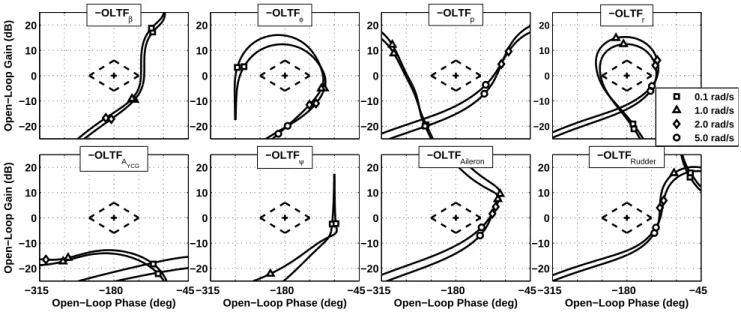
The quoted characteristics are extracted from the magnitude versus phase plot, applied to the transfer function -OLTF. The test consists in a graphical check of these transfer functions against a pre-defined template, which can be modified in ac-cordance with the problem in hand.
Figure 5 (a) presents one example of a case which passes the robustness criterion, while Fig. 5 (b) presents a failed one. The dashed curve is constructed around the critical point, marking the so called robustness boundary. In this case, straight lines connects the±6 db gain margin with the±
In1
In 2
In 3
In n
S 2
S 3
S n S1
ComU 1 ComU
2 U
2
U 1
ComU p U
p
R 1
R2
R t
. . . . . .
. . .
. . . . . .
1
Actuation Models
AFCS
Sensor Models Aircraft Model
(Rigid −Body EQM , Atmosphere , Aerodynamic and Propulsion )
1
Figure 4: Illustration of the building up of one OLTF
−315 −180 −45
−20 −10 0 10 20
(b)
Open−Loop Phase (deg)
Open−Loop Gain (dB)
−315 −180 −45
−20 −10 0 10 20
(a)
Open−Loop Gain (dB)
Open−Loop Phase (deg)
0.1 rad/s 0.5 rad/s 1.0 rad/s 5 rad/s
Figure 5: Magnitude Versus Phase Plot - (a) Success and (b) Fail in the Robustness test
As already mentioned, this robustness check is a widespread procedure employed in the aircraft industry. Examples em-ploying a similar robustness check methodology can be found in (Gangsaas, Blight and Caldeira, 2008; Gangsaas
et al., 2008; Garteur, 1996). Nevertheless, there are issues on this method, which are discussed in the sequence.
The basic concept behind this process is the Nyquist Stabil-ity Criterion (Ogata, 2002), applied to SISO systems. The robustness boundary is set as the region, around the critical point, that shall be avoided. The further is the−OLT F plot to the critical point, the more robust is the closed loop sys-tem.
This concept, which is the same as the gain and phase mar-gin check, is a powerful tool, which can be readily ap-plied to any SISO system. Applying this to the described
OLT F s, extracted out from a MIMO system, is an
extrap-olation which can present issues (Skogestad and Postleth-waite, 2007). Problems may arise since this concept assumes that each loop is modified without any perturbation on the other loops. One particular example where this assumption is valid is the case where there is either an unknown scale factor or an unknown additional time delay applied to only only one of the sensors signals. However, this assumption is not valid in the general case, because a model inaccuracy tends to affect all the loops simultaneously.
−20 −10 0 10 20
−OLTFβ
Open−Loop Gain (dB) −20
−10 0 10 20
−OLTFφ
−20 −10 0 10 20
−OLTFp
−20 −10 0 10 20
−OLTF
r
−315 −180 −45 −20
−10 0 10 20
−OLTFA
YCG
Open−Loop Gain (dB)
Open−Loop Phase (deg)
−315 −180 −45 −20
−10 0 10 20
−OLTFψ
Open−Loop Phase (deg)
−315 −180 −45 −20
−10 0 10 20
−OLTFAileron
Open−Loop Phase (deg)
−315 −180 −45 −20
−10 0 10 20
−OLTFRudder
Open−Loop Phase (deg)
0.1 rad/s 1.0 rad/s 2.0 rad/s 5.0 rad/s
Figure 6: Magnitude Versus Phase Plot -ψhold/ψcapture control law
As an illustration of this approach, Figure 6 provides the magnitude versus phase plots of theψhold/ψcapture con-trol law. The two curves on each plot represent the two mass configurations of Table 1.
Nonetheless, no mathematical proof can be given by this ap-proach. One elegant procedure to overcome this weakness can be achieved by using the structured singular value, called hereµ∆. This approach will be further discussed in Section
5.
4.2
Robust Performance
A solution is considered to possess nominal performance (NP) if the error between the regulated variables and their respective set-points are kept inside a pre-defined limit, even under the maximum expected disturbances.
The adopted nominal performance test consists in first as-sembling the frequency responses of the SISO systems, cor-responding to all aircraft inputs and regulated variables, fol-lowing the idea illustrated in Fig. 7 for inputU1. The
subse-quent step is to compare the magnitude plots of these SISO systems against defined upper boundaries. The overall sys-tem is regarded to have nominal performance if the described plots are all below their respective upper limits.
A robust performance test consists in performing the same checking on the extremes of the mass and CG envelope for each given flight condition. It can also be decided to add a grid of aircraft models with either delay or scale factor per-turbations applied to its inputs and outputs. Each point of
this gridding shall be inside the space of all possible delay and scale factor variations.
Two issues arise in using this robust performance test. The first one is that the number of models to be tested increases to a prohibitive amount as the number of uncertain parameters increases. The second issue is that no mathematical certainty can be given when following this approach, even when the number of point in the grid is made extremely refined. This is so because a worse case can be located in between two points of the chosen grid.
The concept ofµ∆, which is discussed in Section 5, can be
applied to better assess the robust performance of the AFCS.
5
COMPLETING
THE
ROBUSTNESS
TEST
There is an extensive amount of publications about linear fractional transformations (LFT) and µ (Chenglong, Xin and Chuntao, 2010; Hsu et al, 2008; Menon, Bates and Postlethwaite, 2007; Menon et al, 2009; Pfifer and Hecker, 2011; Natesan and Bhat, 2007; Yun and Han, 2009; Zhou et al, 2007). The objective of this section is to make use of the well-established characteristics of these tools, with the final target of proposing one set of tests to measure the robust sta-bility and performance.
In 1
In 2
In 3
In n
S 2
S 3
S n S
1
ComU 1 ComU2 U2
U 1
ComU p U
p
R 1
R2
R t
. . . . . .
. . .
. . . . . .
w 1 y
1
1
Actuation Models
AFCS
Sensor Models Aircraft Model
(Rigid −Body EQM , Atmosphere , Aerodynamic and Propulsion )
1
Figure 7: One of the SISOs systems used for measuring the nominal performance of the feedback system.
quoted robustness tests. For illustration purposes, the defined tests are then applied to theψhold/ψcapture control law.
5.1
Short review of LFT and
µ
The starting point for the robustness analysis is a system rep-resentation in which the uncertain perturbations are lumped into a block diagonal matrix, as represented in Eq. (1).
∆ =diag{∆i} (1)
When following this approach, for the particular case of con-trol law analysis, it is sufficient to use theN∆−Structure (Skogestad and Postlethwaite, 2007) depicted in Fig. 8.
w z
y∆ u∆
1
N ∆
1
Figure 8:N∆−Structure for robust performance analysis
In Fig. 8,Nis the generalized plant, including the controller, wis a vector representing the exogenous inputs (which can be weighted) andz is a vector representing the exogenous output (which may also be weighted). The∆matrix, repre-senting the system perturbations, is built in a way to satisfy
k∆k∞≤1.
The transfer function matrix fromwtoz,z=F w, is related toNand∆by an upper LFT, as shown in Eq. (2).
F = Fu(N,∆)
∆
=
∆
= N22+N21∆ (I−N11∆)
−1
N12
(2)
where theN matrix is partitioned as in Eq. (3) to be com-patible with∆.N22represents the nominal transfer function
fromwtoz(Skogestad and Postlethwaite, 2007).
N =
N11 N12
N21 N22
(3)
The definition of the structured singular value of a complex matrix M, for the allowed structure∆, is presented in Eq. (4).
µ(M)−1 ∆= min{σ¯(∆)|det (I−M∆) = 0
for structured ∆} (4)
Clearly µ(M)depends not only onM, but also on the al-lowed structure for∆. For this reason, it is preferable to use the notationµ∆(M). In words,µ∆(M)is the reciprocal of
the smallest structured ∆(withσ¯ as the norm) that can be found and that can makes the matrix(I−M∆)singular.
In 1
In 2
In 3
In n
S 2
S 3
S n S
1
ComU 1 ComU
2 U
2
ComU p U
p
R 1
R 2
R t
. . . . . .
. . .
. . . . . .
w 1 y
1 z
1
U 1
1
Actuation Models
AFCS
Sensor Models Aircraft Model
(Rigid −Body EQM , Atmosphere , Aerodynamic and Propulsion )
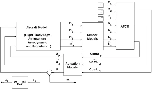
W
pU1(s) 1
Figure 9:NU
1
22 component of theN
U
1transfer matrix
on this section, it is possible to formulate the robust stability (RS) and the robust performance (RP) in terms of the con-ditions stated in Eq. (5) and (6) (Skogestad and Postleth-waite, 2007).
RS⇔µ∆(N11)<1, ∀ω, and NS satisfied (5)
RP ⇔
µ∆˜(N)<1, ∀ω,
˜ ∆ =
∆ 0
0 ∆P
,
and NS satisfied
(6)
where NS means nominal stability, which is verified by the simple check of all the closed loops poles real part. ∆P is a full complex matrix, which has dimension compatible with the vectorswandz.
5.2
Proposed tests based on
µ
The RS test is based on Eq. (5), while the RP test is based on Eq. (6). To use these equations, it is first necessary to put the control problem into the structure of Fig. 8.
The selected strategy consists in assembling one set ofNs. The componentN11 is common to all elements of this set.
TheN22partition is always a SISO model.
Figure 9 shows NU1
22, which corresponds to the weighted
transfer function of an external disturbance onU1to the
ac-tualU1. The weight WpU1 establishes how fast the
distur-bance is to be removed by the feedback component.
The transfer function1/WpU1 represents an upper limit to
the transfer function ofw1toy1, considering all the possible
perturbations. The general shape of1/WpU1 is a wash-out
filter.
Following the same procedure,NUp
22 is established for all
air-craft inputs. The weight selected for each airair-craft input de-pends on the required attenuation, per frequency, of all the external disturbances on the given input. In other words, the weight characteristics for each aircraft input become an en-gineering requirement.
Additionally, NRVp
22 is also created, corresponding to the
weighted transfer function of an external disturbance onRVp to the actual RVp. In this case, the weight choice is also based on the engineering requirement dictating how fast the external disturbance shall be removed from the given regu-lated variable.
For the example of theψ hold/ψ capture control law, the regulated variables areψ andβ and the aircraft inputs are aileron and rudder. This means that, for this particular case, the RP test is based on the analysis of four LFTs:µ∆˜(Nβ),
µ∆˜(Nψ),µ∆˜(NAileron)andµ∆˜(NRudder).
As already mentioned, theN11component is the same for all
1. Add the perturbation weight described in Fig. 10 (a) for all aircraft outputs which have phase type inaccuracy. The value ofτd represents the maximum expected ad-ditional delay, in seconds, that might be present on the particular signal;
2. Add the perturbation weight described in Fig. 10 (b) for all aircraft outputs which have scale factor type in-accuracy. The value offSignalrepresents the maximum expected scale factor that might be present on the par-ticular signal;
3. Repeat items number 1 and 2, but now for all of the aircraft inputs.
In 1 In
1 (a)
(b)
2
1 (1/f
Signal) − 1 TF
delay(s) δdIn1
δfIn1 2
1
Figure 10: Perturbation due to (a) delay inaccuracy and (b) scale factor inaccuracy
In Fig. 10,δdIn1represents an uncertain complex gain and
δf In1represents an uncertain real gain. The magnitudes of
bothδdIn1 andδf In1are limited to be less than or equal to
1. The transfer functionT Fdelay(s)has the general format described in Eq. (7) (Skogestad and Postlethwaite, 2007).
T Fdelay(s) =
2τds τds+2
τ2
ds2+2(0.838)2.363τds+(2.363)2 τ2
ds2+2(0.685)2.363τds+(2.363)2
(7)
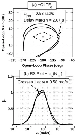
For the particular case where it is assumed the existence of inaccuracy in only one loop, it can be shown that the re-sult of RS viaµleads to the same conclusion of the OLTF phase and gain margin check. As an example of this fea-ture, Figure 11(a) shows the magnitude versus phase plot of
the−OLT Fφ, which shows a phase margin of 69.2 deg at
0.58rad/s, corresponding to an equivalent delay margin of
2.07 s. Figure 11(b) shows theµ∆(N11), considering that the
only source uncertainty is the delay on theφloop and that the maximum expected inaccuracy corresponds toTSignal= 2.07 s. The plot ofµ∆(N11)crosses 1 at the phase margin
frequency provided by the−OLT Fφplot.
Similar results are achieved considering phase perturbations on the other loops, as well as gain factor perturbations.
−315 −270 −225 −180 −135 −90 −45
−20 −10 0 10 20 30
(a) −OLTFφ
Open−Loop Gain (dB)
Open−Loop Phase (deg) ω
pm = 0.58 rad/s Delay Margin = 2.07 s
10−2 10−1 100 101 102
0 0.5 1
1.5 (b) RS Plot − µ∆(N11)
ω [rad/s]
µ
Crosses 1 at ω = 0.58 rad/s
Figure 11:µValidation
Therefore, when it is considered inaccuracy in only one loop at each time, the conclusion based on theµanalysis produces the same result as the margins checks of theOLT F. How-ever, theµanalysis allows the additional check of simultane-ous perturbations in a straightforward manner.
5.3
Results of
ψ
hold
/ψ
capture control
law
In order to exercise the concepts presented in this section, the ψ hold/ψ capture controls law was tested, considering the maximum model inaccuracies as described on Table 5.
Table 5: Model inaccuracy factors
Signal τd[s] fSignal[ADM]
ψ 0.020 1.00
φ 0.020 1.00
p 0.010 1.00
r 0.010 1.00
AY CG 0.010 1.00
β 0.020 1.00
Aileron 0.010 1.15
0 0.2 0.4 0.6 0.8 1
RS Plot − µ∆(N
11)
µ
0 0.2 0.4 0.6 0.8 1
RP Plot Psi − µ∆ (Nψ)
10−2 10−1 100 101 102 0
0.2 0.4 0.6 0.8 1
RP Plot Psi − µ∆(Nβ)
ω [rad/s]
µ
10−2 10−1 100 101 102 0
0.2 0.4 0.6 0.8 1
RP Plot Psi − µ ∆(NAileron)
ω [rad/s]
~
~ ~
Figure 12:µresults
The selected performance weights have the general format described in Eq. (8). The parameters values for each specific weight are given in Table 6.
Wp(s) =
1
ap
τ
ps+ 1 τps
(8)
Table 6: Performance weight parameters
Signal ψ β Aileron
τp[s] 10 1.5 1.0
ap[ADM] 1.3 2.0 2.0
In this design, the rudder demand is obtained exclusively from theβfeedback components (proportional, integral and derivative components ofβ). For this reason,Nβis the same as NRudder. The final results are shown in Fig. 12. One important note is that eachµplot shown on this article is in fact an upper bound on the respectiveµ.
5.4
Discussion
The current industrial method has the drawback of assuming that the model inaccuracy is applied in only one of the loops. This can be the case sometimes, but, in the general situation, there may be errors in each of the aircraft inputs or sensor in-puts. The actual error can be the result of any of the possible combinations.
The proposed additional tests, based on the concept ofµ∆,
allows the determination, in one go, of the worst combination
of the possible errors, in terms of hampering the final stability and performance.
The proposed final procedure combines the two presented methodologies. The reason is that -OLTFs magnitude ver-sus phase plot can be used not only as robustness measure-ment tool of individual loops inaccuracy, but also as a in-strument for guiding the control law loop shaping, obtained via phase shift and/or gain increase/decrease of the -OLTFs. One important result of the proper OLTFs loop shaping is the fact that the damping of the closed loop poles are intimately linked with the proximity of these curves to the critical point.
The supplementary tests, based onµ∆, work as a
comple-ment for the current methodology, since it fulfills the exist-ing gap. It does not provide the same aid in terms of in-dicating the best strategy for the control law loop shaping, but it provides the correct assurance of robust stability and performance for the most common situation, where the inac-curacies may happen simultaneously in multiple loops.
Another interesting usage of theµ∆robust performance test
is that it allows the arbitration of the best control law among a set of control laws, which were generated following different design approaches.
6
CONCLUSIONS
step by step procedure was presented, illustrating the use of the method.
ACKNOWLEDGEMENTS
The authors would like to thank the Brazilian agency CNPq (research fellowships) and the Brazilian companies Embraer and Mectron for their support.
REFERENCES
Araki, M. and Taguchi, H. (2003). Two-Degree-of-Freedom PID Controllers, International Journal of Control, Au-tomation, and Systems 1(4):401-411.
Chenglong, H., Xin, C. and Chuntao, L. (2010). Application of Mu-Analysis for Evaluating the Robustness of RLV’s Flight Control System, IEEE International Conference on Electrical and Control Engineering (ICECE 2010), Wuhan, pp. 5027-5030.
Cook, M. V. (2007). Flight dynamics principles, Butterworth-Heinemann, Oxford, UK.
DoD (1990). Flying Qualities of Piloted Aircraft, Military Standard MIL-STD-1797A.
Gangsaas, D., Blight, J. and Caldeira, F. (2008). Control Law Development for Aircraft: An Example from Industry Practice. Tutorial Session, American Control Confer-ence (ACC), Seattle, USA.
Gangsaas, D., Hodgkinson, J., Harden, C. Seeed, N. and Kaiming, C. (2008). Multidisciplinary control law de-sign and flight test demonstration on a business jet, Pa-per AIAA 2008-6489. AIAA Guidance, Navigation and Control Conference and Exhibit, Honolulu, USA.
GARTEUR (1996). Robust Flight Control Design Challenge Problem Formulation and Manual: The High Incidence Research Model (HIRM), GARTEUR/TP-088-4.
Hsu, K., Vincent, T., Wolodkin, G., Rangan, S. and Poolla, K. (2008). An LFT approach to parameter estimation, Automatica 44(12): 3087-3092.
Menon, P.P., Postlethwaite, I., Bennani, S., Marcos, A. and Bates, D.G. (2009). Robustness analysis of a reusable launch vehicle flight control law, Control Engineering Practice 17(7):751-765.
Menon, P.P., Bates, D.G., and Postlethwaite, I. (2007). Non-linear robustness analysis of flight control laws for highly augmented aircraft, Control Engineering Prac-tice 15(6):655-662.
Natesan, K. and Bhat, M.S. (2007). Design and flight test-ing of Hinf lateral flight control for an unmanned air vehicle, IEEE International Conference on Control Ap-plications (CCA 2007), Singapore, pp. 892-897.
Ogata, K. (2002). Modern Control Engineering, Prentice Hall, Upper Saddle River, New Jersey, USA.
Pamadi, B. N. (2004). Performance, stability, dynamics, and control of airplanes, American Institute of Aeronautics and Astronautics, Inc., Reston, Virginia, USA.
Pfifer, H. and Hecker, S. (2011). Generation of Optimal Lin-ear Parametric Models for LFT-Based Robust Stabil-ity Analysis and Control Design, IEEE Transactions on Control Systems Technology 19(1): 118-131.
Phillips, W. F. (2004). Mechanics of flight, John Wiley and Sons, Hoboken, New Jersey, USA.
Roskam, J. (2003). Airplane Flight Dynamics and Auto-matic Flight Controls I and II, Design Analysis Re-search (DAR) Corporation, Lawrence, Kansas, USA.
Roskam, J. and Lan, C.-T. E. (2003). Airplane aerodynam-ics and performance, Design Analysis Research (DAR) Corporation, Lawrence, Kansas, USA.
Silva, A.S.F. (2009). An approach to design feedback trollers for flight control systems employing the con-cepts of gain scheduling and optimization, Master The-sis, Instituto Tecnológico de Aeronáutica (ITA), Brazil. Available from http://www.bd.bibl.ita.br/tesesdigitais/ lista_resumo.php?num_tese=000552692 (last accessed on Feb 04th, 2011).
Skogestad, S. and Postlethwaite, I. (2007). Multivariable Feedback Control – Analysis and Design, John Wiley and Sons, Inc., New York, USA.
Stevens, B. L. and Lewis, F. L. (2003). Aircraft Control and Simulation, John Wiley and Sons, Inc, New York, USA.
Yechout, T.R. and Morris, S.L. (2003). Introduction to air-craft flight mechanics: performance, static stability, dy-namic stability, and classical feedback control, Ameri-can Institute of Aeronautics and Astronautics, Inc., Re-ston, Virginia, USA.
Yun, H. and Han, J. (2009). Robust flutter analysis of a non-linear aeroelastic system with parametric uncertainties, Aerospace Science and Technology 13: 139-149.