The general purpose analog computer and recursive functions over the reals

(1)

UNIVERSIDADE T´

ECNICA DE LISBOA

INSTITUTO SUPERIOR T´

ECNICO

The General Purpose Analog Computer

and

Recursive Functions Over the Reals

Daniel da Silva Gra¸ca

MSc thesis

(submitted)

July 2002

(2)

(3)

O Computador Anal´ogico e Fun¸c˜oes Reais Recursivas

Nome: Daniel da Silva Gra¸ca

Curso de Mestrado em: Matemática Aplicada Orientador: Doutor José Félix Gomes da Costa Provas conclu´ıdas em:

Resumo: Pretende-se analisar na presente disserta¸cão diversos modelos mate-máticos de computa¸cão analógica.

Come¸ca-se por analisar o primeiro modelo conhecido deste tipo, o Computa-dor Analógico (GPAC, abreviatura do inglês). São descritos os principais resul-tados existentes para este modelo, sendo também apresentada uma abordagem alternativa. É mostrado que esta nova abordagem origina um modelo mais ro-busto que o GPAC, mantendo, no entanto, as suas principais propriedades, tais como a equivalência com fun¸cões diferencialmente algébricas. Introduzem-se também novos conceitos que julgamos relevantes, tais como o procedimento de inicializa¸cão e a no¸cão de GPAC efectivo.

Seguidamente, o nosso estudo incide sobre a teoria das fun¸cões reais recur-sivas, uma teoria análoga à teoria clássica das fun¸cões recurrecur-sivas, em que as fun¸cões são consideradas sobre o conjunto dos reais, em vez do conjunto dos naturais. Propõem-se novas classes de fun¸cões, relacionando-se estas com as principais classes da teoria clássica, incluindo a Hierarquia Aritmética. Além disso, mostram-se ainda rela¸cões entre as fun¸cões reais recursivas e fun¸cões ge-radas por modelos semelhantes ao GPAC.

Palavras-chave: Computa¸cão analógica, computador analógico, equa¸cões di-ferenciais, sistemas dinâmicos, fun¸cões recursivas, hierarquia aritmética.

(4)

The General Purpose Analog Computer and Recursive Functions Over the Reals

Abstract: The purpose of the present dissertation is to analyze various math-ematical models of analog computation.

This work starts by analyzing the first known model of this kind, the Gen-eral Purpose Analog Computer (GPAC). We present the existing results for the GPAC and propose an alternative approach. We show that this approach origi-nates a more robust model than the GPAC, maintaining its principal properties such as the equivalence with differentially algebraic functions. We also introduce new concepts such as the initialization procedure and effective GPACs that we think to be relevant.

We pursue our study with the theory of recursive functions over the reals, a similar theory to the classical theory of recursive functions, proposing new classes of functions and relating them with the main classes of the classical theory, including the Arithmetical Hierarchy. We also show relations between recursive functions over the reals and functions generated by models similar to the GPAC.

Key-words: Analog computation, general purpose analog computer, differen-tial equations, dynamical systems, recursive functions, arithmetical hierarchy.

(5)

Acknowledgments

Firstly, I want to thank my advisor, J. F´elix Costa, for its dedication and guidance during the elaboration of this thesis. The constant support and mo-tivation that he provided were essential for the determination of the course of this work. And with its energy and enthusiasm, he was also able to present me a more realistic perspective of research that I had, certainly improving my skills in this domain.

I would also like to thank the Section of Computer Science of the Department of Mathematics at IST/UTL for the assistance and support provided whenever needed. I also wish to thank my colleagues at the Department of Mathematics of the University of Algarve for their help in several occasions.

I must also express my gratitude to the Center for Logic and Computation and, in particular, to Am´ılcar Sernadas, for the opportunities that I had to expose my work in the Theory of Computation Seminar.

Many people helped me with useful discussions and suggestions, while doing this work. In particular, I wish to thank Manuel Campagnolo, Stefan Samko, J. Sousa Ramos, Hermenegildo Borges, Celestino Coelho, and Cristopher Moore. I also wish to thank Diana Rodelo for the improvements done in some parts of this text.

Finally, I wish to give very special thanks to my family, for their presence and unconditional support.

(6)

(7)

Introduction

The quest for understanding nature has long been one of the biggest challenges of human kind. The search for answers has lead to the creation of a diversity of models trying to explain and model different aspects of nature.

Meanwhile, a tremendous effort has been made with the objective of con-trolling natural phenomena in order to serve human needs. Nowadays, more than ever, technology is a key factor within human society.

Hence, the demand for machines that could simulate some aspects of the physical world appeared naturally, in order to understand and model it. Sev-eral computational models appeared to perform this task, but discrete (digital) models gained a rapid prominence.

Digital computation has been, since the thirties, the most important com-putational model, mainly due to the unifying work of Turing. Turing clarified the notion of algorithm, giving it a precise meaning, and introduced a coherent framework for discrete computation. In a short time, new results showing the relations of his model with other approaches, such as recursive functions (in the sense of Kleene), originated in a natural way consistent theoretical basis to stan-dard computation theory. Meanwhile, with the rapidly growing needs of various fields such as physics, engineering, etc., to make enormous quantities of calcula-tions and information processing, many times beyond human capabilities, new computing devices were developed and improved. With these new technologies, digital computers improved dramatically in speed, size and accuracy, until the present date. Hence, it is not difficult to understand why discrete computation became today’s main computational paradigm.

Nevertheless, computers need not to be digital. In fact, the first computers were analog computers. In an analog computer, the internal states are continu-ous, rather than discrete as in digital computation. The first analog computers were especially well suited to solve ordinary differential equations and were ef-fectively used to solve many military and civilian problems during World War II (e.g. gunfire control) and in the fifties and sixties (e.g. aircraft design). Unfortunately, because of the inexistence of a coherent theoretical basis to ana-log computation and the fact that anaana-log computers technoana-logy almost didn’t improve when compared with its digital counterpart in the last half century, analog computation was about to be forgotten with the emergence of digital computation.

(10)

in-Introduction

terest. The search for new models that could provide an adequate notion of computation and complexity for the dynamical systems that are currently used to model the physical world contributed to change the situation. However, rel-atively little work exists on a general theory for analog computation, and this still seems far away. Nevertheless, this is a potentially rich and fertile field. In analog computers, each real is handled exactly and is considered to be an intrin-sic quantity, whereas in digital computers it is represented (and approximated) by strings of digits. Hence, it seems that analog computation is better suited for studying notions of computability and complexity for continuous dynamical systems.

Generally speaking, any computational model can be seen as a dynamical system. The main property that distinguishes analog models from digital ones is the use of a continuous state space [Sie99].1 _{Besides this feature there is no}

agreement upon the properties that characterize an analog model of computa-tion. However, in this dissertation, we will say that a model of computation is digital if its space of states is discrete and analog otherwise.

Recent research [Moo90, Koi93, KCG94, KM99] shows that Turing machines, when converted into discrete dynamical systems, can be embedded in analog systems. Hence, we could see analog computation as an extension of digital computation. Moreover, in this fashion, we get a physical meaning to the Turing machine that cannot be obtained with the classical description.

We can also find common paradigms both to digital and analog computation, such as neural networks. Neural networks first appeared as discrete models [MP43], proposed by McCulloch and Pitts, but we can now find significant research in analog neural networks. For instance, Siegelmann and Sontag [SS94] were able to show how to simulate Turing machines with analog neural networks. Although analog computation is certainly in its infancy, current research suggests some lines of work. Some analog models may be seen as high di-mensional dynamical systems (highly parallel models), e.g. neural networks, and others may be seen as low dimensional dynamical systems (e.g. [Moo90, KCG94, KM99]). On the other hand, we may classify analog models as discrete time models (e.g. [Sie99]) or as continuous time models (e.g. [Orp95]). How-ever, this is not a rigid characterization and it is possible to find hybrid models (e.g. [Bra95]). In this thesis we will be mainly concerned with continuous time models.

We will now briefly refer the contents of this dissertation. The initial pur-pose was to develop and explain the ideas presented in [Moo96]. In his paper, Moore introduced a recursion theory over the reals and presented some results establishing links with the classical recursion theory and also with a continu-ous time model of analog computation, the General Purpose Analog Computer (GPAC).

Unfortunately, these results presented some gaps and, hence, the primary goal of this thesis is precisely to provide an adequate framework to obtain, whereas possible, similar results to those presented by Moore. In particular,

(11)

Introduction

we are interested in presenting connections between recursive functions over the reals and functions generated by the GPAC. Nevertheless, while working on this topic, some problems not referred in existing literature (at least to our knowledge) appeared and a major revision of the GPAC was needed for our purposes. Therefore, this dissertation is roughly divided in two parts. The first part (corresponding to chapters 1 and 2) is dedicated to the study of the GPAC and the second part (chapter 3) is dedicated to recursive functions over the reals. The contents of each chapter are as follows.

In Chapter 1 we introduce the reader to the classical theory about the GPAC. We explain its underlying motivations and present an outline of the previous work done on the GPAC. This is basically an introductory chapter to the next chapter.

In chapter 2 we start by analyzing some problems that appear in the scope of the GPAC and we present an alternative model for it (the feedforward GPAC: FF-GPAC) that solves most of the problems referred for the GPAC. The rest of the chapter is devoted to the task of showing that the FF-GPAC model is more robust than the GPAC, but that still preserves the fundamental properties (equivalence with differentially algebraic functions). The last two sections may appear uninteresting but they will be important for the main result that we present in Chapter 3.

The third chapter is devoted to recursion theory over the reals. It is a mixture of existing theory (mainly contributions from C. Moore, M. L. Campagnolo, and J. F. Costa) and of new results that we propose in this thesis. It may be used as an introduction to the topic of recursive functions over the reals. The importance of results in this section depends on the point of view. In sections 3.1, 3.2, and 3.3, the existing theory is present and new results are added. Several connections between recursive functions over the naturals and recursive functions over the reals are established. If the reader is mainly interested in recursion theory, these are probably the most interesting sections. In sections 3.4 and 3.5, we establish full connections between some particular subclasses of recursive functions over the reals and the FF-GPAC model. We believe that this is an important result because it shows that it is possible to establish connections between recursive functions over the reals and a model based on circuits (the FF-GPAC).

(12)

(13)

Chapter 1

Preliminaries

1.1 Shannon’s Work

In this section we will go to the origins of analog computation with the pioneer work of Claude Shannon on the so-called General Purpose Analog Computer (GPAC).1 _{In essence, this is a mathematical model of an analog device, the}

dif-ferential analyzer. The fundamental principles for this device were first realized by Lord Kelvin in 1876 [Bus31]. Working with an integrating device conceived by his brother James Thomson, he had the idea of connecting integrators to solve differential equations.

A mechanical version of the differential analyzer was first developed by V. Bush and his associates at MIT in 1931 [Bus31]. Many mechanical difficulties were overcome by ingenious solutions. However, the inherent difficulties of the mechanical devices, due to mechanical restrictions, limited the speed of these differential analyzers and originated colossal machines.

The introduction of electronic differential analyzers was able to overcome these problems to a great extent. But this was not enough to compete with emergent digital computers.

Differential analyzers were typically used in the thirties and forties to com-pute functions, especially to solve ordinary differential equations (ODEs). Their continuous nature allowed the direct simulation of a solution from a given sys-tem of ODEs.2 _{Hence, comparatively to standard procedures that basically use}

a discrete version of time (i.e., the independent variable) in order to approximate the solution (with the inherent errors introduced in these processes), differen-tial analyzers permitted faster solutions with increased precision at that time.

1_{This name is somewhat misleading. This is not a general purpose device capable of}

handling all kinds of analog computations in a similar way as a universal Turing machine do. And it is not known whether it exists some general machine that can do all the computations that every GPAC can. Nevertheless, this is the usual designation in the field and we will hence keep it.

2_{In general, this system of ODEs must satisfy some conditions in order to be simulated by}

a differential analyzer. However, experience rapidly demonstrated that a differential analyzer could solve many useful systems of ODEs.

(14)

Preliminaries

As an example, the Rockeffeler Differential Analyzer (designed by V. Bush and operational for the war effort in 1942) could solve an ODE up to order 18, being able to produce results to at least 0.1 percent accuracy [Bow96, p. 8].

A differential analyzer may be idealized as a General Purpose Analog Com-puter that basically is a model consisting of several (finite number) intercon-nected units, i.e., a circuit.3

Figure 1.1.1: A disc type integrator device. Figure taken from [Bur71] with permission of Dover Publications, Inc.

There are some restrictions in the way in which these units are connected, but in general it is a quite liberal model. After having the circuit properly set up (i.e., after connecting in an appropriate way all the units), the computation can be started. The inputs of the circuit will be applied to the inputs of units not connected to any output.

When we introduce some input into the circuit, each unit will respond cor-respondingly to this input, generating some kind of output. We may pick some of these outputs to be the result of the computation (that we will refer as the functions generated or computed by the GPAC). In mechanical differential an-alyzers, the quantities involved in the computation are usually represented by the rotation of shafts, and in a electronic differential analyzer they are usually represented by electric voltages.

The units used in a GPAC are the following:

• Integrator : a two-input, one-output unit with a setting for initial

condi-3_{More formally, it is sufficient for our purposes to consider a circuit as being a 7-tuple}

(V, X, Y, E, S, σ, h), where V is a non-empty set (set of units), X is a set satisfying X ∩ V = ∅ (set of inputs), Y ⊆ V ∪ X (Y denotes the set of outputs), S is a set satisfying S ∩ (V ∪

X ∪ E) = ∅ (set indicating the type of the units), σ : V → S is a function such that dom(σ) = V (it assigns each unit to its type), h : S → N (we consider 0 ∈ N) is a function

such that dom(h) = S (it indicates the number of inputs associated to each type of unit), and

E ⊆ (V ∪X)×V ×(N−{0}) satisfies the following conditions: if (a, b, n) ∈ E then n ≤ h(σ(b))

and if (a1, b, n), (a2, b, n) ∈ E then a1 = a2. If (a, b, n) ∈ E we say that the output of a is

connected to the nth input of b. We consider units only with one output because, for our

purposes, we may replace a unit with k outputs by k units, each with one output (keeping the same number of inputs).

(15)

1.1 Shannon’s Work

tion. If the inputs are unary functions u, v, then the output is the Riemann-Stieljes integral λt.R_t0tu(x)dv(x) + a, where a and t0are constants defined

by the initial settings of the integrator.

• Constant multiplier : a one-input, one-output unit associated to a real number. If u is the input of a constant multiplier associated to the real number k, then the output is ku.

• Adder : a two-input, one-output unit. If u and v are the inputs, then the output is u + v.

• Multiplier : a two-input, one-output unit. If u and v are the inputs, then the output is uv.

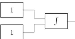
• Constant function: a zero-input, one-output unit. The value of the output is always 1.

×k ku

u

A constant multiplier unit associated to the value k

+ v u u+v An adder unit × v u uv A multiplier unit 1 1

A constant function unit Figure 1.1.2: Representations of different types of units in a GPAC.

We will also take from here the following conventions: except indicated other-wise, the inputs of a unit appear on the left and the outputs appear on the right (see figures 1.1.2 and 1.1.3); in an integrator the input corresponding to the in-tegrand is on the top and the input corresponding to the variable of integration is on the bottom (see fig. 1.1.3).

R

v u

λt.Rt

t0u(x)dv(x) Figure 1.1.3: An integrator unit

As in the differential analyzer, we require that two inputs and two outputs can never be interconnected. We also demand that each input is connected to, at most, one output (but each output can be connected to several inputs).

These are natural restrictions that still allow considerable freedom to make connections. We can make circuits with feedback, generating in this way a rich set of functions. Of course, we could add other types of units (and this was actually done in practice), obtaining possibly different behaviors. But circuits

(16)

Preliminaries

are, in general, difficult models to deal with. So, we won’t take this approach here and we will only analyze the circuits described above. Nevertheless, we think that it is a very interesting question to see what happens when new units are added. Circuits are widespread used, e.g. in engineering, and even digital computers are designed using circuits instead of thinking them as Turing machines.

Remark 1.1.1 Notice that an output of a GPAC can be considered as being the output of an integrator. In fact, suppose that the output y is the output of some unit Ak. Hence, we may introduce a new integrator and connect the

input associated to the variable of integration to the output of Ak, and the

input associated to the integrand to a constant function unit. If we set the initial condition of the output of the integrator to be y(t0), the output of this

integrator will be precisely y.

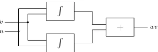
Remark 1.1.2 Note that we do not need the multiplier unit. In fact, using the formula of integration by parts (for definite integration), we obtain

u(t)v(t) = Z t t0 u(x)dv(x) + Z t t0 v(x)du(x) + u(t0)v(t0).

So, uv can be computed by the circuit of figure 1.1.4.

R R + u v uv q q

Figure 1.1.4: A circuit that computes uv.

In the circuit, we can take as initial conditions y1(t0) = u(t0)v(t0) and

y2(t0) = 0 for the outputs of the integrators at the bottom and at the top,

respectively. Note that this actually only works when the Riemann-Stieljes integrals are defined. So, if we add other types of units as building components of the GPAC, this approach may fail.

Notice that in the above description of the units, a parameter t appears. Although it usually appears when defining these kind of circuits, its function is somehow unclear. In his seminal paper [Sha41], Shannon considers t to be some independent variable that is inputted into the circuit. He also considers that more than one independent variable can be inputted, say t1, ..., tn. He even

manages to state some results for this case. However, these results are based in the assumption that the variables are independent, which appear not to be the case for differential analyzers. If we think in terms of a physical device, all the inputs are functions of time and they don’t have to be independent (even if we don’t know their actual relationships). So, we believe that this is not an appropriate model for working with differential analyzers with more than one input.

(17)

1.1 Shannon’s Work

In the description of differential analyzers given in [Pou74] we find the ideas reported above: “The functions generated by an electronic differential analyzer are functions of time...” (p. 9) and “The functions generated by a mechanical differential analyzer are also functions of time” (also p. 9). Nevertheless, when Pour-El defines the GPAC she says: “Note that our functions are not necessarily functions of time” (p. 10) and in a footnote of page 11, she continues: “An obvious modification of this can be made when dealing with functions of more than one variable. Simply require that precisely one of the independent variables be applied to each input not connected to an output.” So, when dealing with more than one variable, she actually works with independent variables.

However, even if time is our independent variable, we cannot input it directly to, e.g. an electronic differential analyzer. What we actually input is some function x = λt.x(t). For the one variable case, this actually does not make much difference: simply take x as a new independent variable. But for the case of more than one variable, the same does not happen. We are interested to clarify this point to present some results for the case of more than one variable. Little has been made in this domain and, as far as we know, the only results about this case appear in [Sha41].

In order to clarify the problem indicated above, we will suppose that a GPAC can have more than one input, but each input depends on a parameter t that we call the time (although this may not actually correspond physically to time but, e.g. to displacement). Hence, if x1, ..., xnrepresent the inputs, there exist unary

functions (and we are not assuming any special property for them) ϕ1, ..., ϕn

such that x1= ϕ1, ..., xn= ϕn. If we only have one variable, we will often work

with it as it were an independent variable.

This approach is similar to Turing machines, where the computations are done with the increment of one discrete variable, the running time (that usu-ally corresponds to the number of steps that were already performed in the computation).

Although the work presented in [Sha41] contained some gaps, it introduced the main results and tools of the area. In particular, Shannon was the first to note an important connection that we will state in what follows.

Definition 1.1.3 A unary function y is differentially algebraic (d.a.) on some set I if there exists some natural number n, where n > 0, and some n + 1-ary nonzero polynomial P with real coefficients such that

P (x, y(x), ..., y(n)_{(x)) = 0,}

for every x ∈ I.

We now present the first version of an important result, establishing fun-damental links with other fields of mathematics, that was first presented in [Sha41].

Claim 1.1.4 (Shannon) A unary function can be generated by a GPAC if and only if the function is differentially algebraic.

(18)

Preliminaries

This result indicates that a large class of functions, such as polynomials, trigonometric functions, elliptic functions, etc., could actually be generated by a GPAC. As a corollary some functions such as the Gamma function,

Γ = λx. Z _∞

0

tx−1_e−t_dt,

could not be generated (cf. [Car77, pp. 49,50]). Nevertheless, the claim 1.1.4 gives us a nice characterization of the class of functions computed by the GPAC. Unfortunately, the original proof of claim 1.1.4 contained some gaps, as indicated on pp. 13-14 of [Pou74].

1.2 Examples

In order to familiarize the reader with the GPAC, we will give three examples in this section.

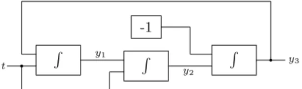
Example 1: We will start by analyzing the circuit represented in figure 1.2.1 (taken from [Cam02]).

R _R R

-1

q q

t _y2 y3

y1

Figure 1.2.1: A circuit that computes both sin and cos.

The box with −1 inside represents a circuit that outputs the value −1. It can be obtained by connecting a constant function unit to a constant multiplier unit associated to the value −1. We can easily see that y1, y2, and y3 are functions

of t satisfying the following system of equations    y0 1= y3, y0 2= y1, y0 3= −y02.

Solving it, we get the solutions expressed by    y1= c1cos +c2sin, y2= c1sin −c2cos +c3, y3= −c1sin +c2cos .

In particular, if we set the initial conditions of the integrators to y1(0) = 1,

y2(0) = 0, and y3(0) = 0, we have y1 = cos, y2 = sin, and y3 = − sin . Hence,

(19)

1.2 Examples

Note that, as indicated in claim 1.1.4, sin and cos are d.a. functions. In fact, sin and cos are solutions of

y00_{+ y = 0.}

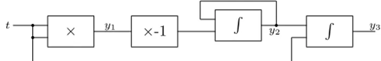
Example 2: Consider the circuit pictured in figure 1.2.2.

R R ×-1 × q q q y1 _y2 y3 t

Figure 1.2.2: A circuit that computes the function with expression Rt

0e−v

2

dv.

Associated to it, we have the following system of equations    y1= λt.t2, y0 2= −y2y01, y0 3= y2.

If we take y2(0) = 1 and y3(0) = 0, we get the following expressions for the

solutions: y1(t) = t2, y2(t) = e−t 2 , and y3(t) = Rt 0e−v 2

dv. Note that y3is a d.a.

function because, for each t ∈ R, 2ty0

3(t) + y300(t) = 0.

Note also that y3is not an elementary function in the following sense (see [CJ89,

p. 261], [Zwi96, p. 352]): its expression cannot be obtained by repeated use of addition, multiplication, division, and composition of the usual functions (power, exponential, trigonometric, and rational functions and their inverses) in a finite number of times. Hence, if we want to calculate the value of y3

for some point t in actual computers, we must apply some procedure such as Simpson’s rule to approximate numerically its value. Nevertheless, as we have just seen, this function can be computed exactly by a GPAC.

Although a primitive of λv.e−v2

is not an elementary function, it is not dif-ficult to show (using polar coordinates) that R_−∞0 e−v2

dv = √₂π. Then we can easily adapt the circuit of figure 1.2.2 to compute the integralR_−∞t e−v2

dv asso-ciated to the Gaussian distribution. This distribution finds many applications in the theory of probability and also in physics (e.g. the Maxwell-Boltzmann distribution of velocities).

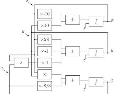
Example 3: Consider the circuit represented in figure 1.2.3.

It is not difficult to see that x, y, and z are solutions of the following system

of ODEs _   x0 _{= −10x + 10y,} y0_{= 28x − y − xz,} z0 _{= −}8 3z + xy.

(20)

Preliminaries

This system describes a simplified model of thermal convection. It was obtained by E. Lorenz in 1963 while studying a rudimentary model of weather. Associated to this system of ODEs, a chaotic dynamical system with a sensitive dependence on initial conditions occurs [McC94, p. 45]. By other words, if we pick two nearby initial conditions, the respective solutions will drive away very fast with the increment of t. ×-8/3 × + R t q z ×-1 ×-1 ×28 + R × q t y ×10 ×-10 + R t q x q q q q q q Q s x Q s y Q s z

Figure 1.2.3: A circuit that computes the solutions of Lorenz’s system of equations. This system is chaotic and has a sensitive dependence on initial parameters.

Hence, if we would like to simulate this system in a computer, we must deal with numbers exactly instead of approximations, as it is done in usual practice, in order to avoid the fast increase of error (because of errors introduced during the calculations). This cannot be done by standard methods in Turing machines (at least without using some unknown properties), but can be implemented in a GPAC.

Then, Turing machines are unable to simulate properly some dynamical systems that can be simulated by the GPAC and can only approximate them up to a certain point in time. Of course, this advantage doesn’t exist in practice: in a physical system there are always some perturbations that will prevent the computation to be exact. Nevertheless, this problem only arises at the practical level, not at a theoretic one, as it appears to be in Turing machines.

1.3 Further Developments

Although the previous notion of GPAC seems fairly intuitive and natural, this is not the notion that people actually refer when talking about the GPAC. The

(21)

1.3 Further Developments

accepted definition is due to Pour-El and was introduced in [Pou74]. As she claims in her paper, Shannon’s proof of claim 1.1.4 is rather incomplete: “A statement somewhat similar to this [claim 1.1.4] appears as part of theorem II [Sha41, p. 342]. We believe that there is a serious gap in the brief proof which appears on the top of p. 343” (footnote in p. 13). And she continues: “For this reason we have found it necessary to proceed along entirely different lines” (footnote in p. 13). “To fix this gap it was not only necessary to change Shan-non’s proof but to introduce the previously mentioned definition...” (footnote in p. 4). So, the main reason for a new definition for the GPAC is to keep some relations of the type indicated in claim 1.1.4.

Let us now present the new definition of Pour-El that we will denominate as theoretic GPAC (or simply T-GPAC). This is not a usual notation, but we prefer to introduce it in order to distinguish this model from the previous one. In the following I will denote a closed bounded interval with non-empty interior. We now introduce the concept of function generated by a T-GPAC for functions of one variable.

Definition 1.3.1 The unary function y is generated by a T-GPAC on I if there exists a set of unary functions y1, ..., yn and a set of initial conditions yi(a) = yi∗,

i = 1, ..., n, where a ∈ I, such that:

1. y = (y1, ..., yn) is the unique solution on I of a system of ODEs of the

form

A(x, y)dy

dx = b(x, y) (1.1)

satisfying the initial conditions, where A(x, y) and b(x, y) are n × n and n × 1 matrices, respectively. Furthermore, each entry of A and b must be linear in 1, x, y1, ..., yn.

2. For some i ∈ {1, ..., n}, y = yi on I.

3. (a, y∗

1, ..., y∗n) has a domain of generation with respect to the equation (1.1),

i.e., there are closed intervals J0, J1, ..., Jn(with non-empty interiors) such

that (a, y∗

1, ..., yn∗) is an interior point of J0×J1×...×Jn and, furthermore,

whenever (b, z∗

1, ..., zn∗) ∈ J0× J1× ... × Jn there exists unary functions

z1, ..., zn such that:

(i) zi(b) = z∗i for i = 1, ..., n;

(ii) (z1, ..., zn) satisfy (1.1) on some interval I∗ with non-empty interior

such that b ∈ I∗_;

(iii) (z1, ..., zn) is unique on I∗.

The existence of a domain of generation indicates that the solution of (1.1) remains unique for sufficiently small changes on the initial conditions. Provided with this definition, Pour-El shows the following:

Theorem 1.3.2 (Pour-El) Let y be a differentially algebraic function on I. Then there exists a closed subinterval I0 _{⊆ I with non-empty interior such that,}

(22)

Preliminaries

She also proves, although with some corrections made by Lipshitz and Rubel in [LR87], the following result:

Theorem 1.3.3 (Pour-El, Lipshitz, Rubel) If y is generable on I by a T-GPAC, then there is a closed subinterval I0 _{⊆ I with non-empty interior such}

that, on I0_{, y is differentially algebraic.}

These results present a valid variation of claim 1.1.4. Hence, because of this important connection, the T-GPAC became a significant model. But why people actually replace the GPAC by the T-GPAC? Let us quote Pour-El: “At first sight the relation between our definition and existing analog computers may seem a bit strange. In order to see that this is a natural generalization which includes existing GPAC we proceed as follows. First we give our definition of [T-GPAC]... This is followed by a discussion of a preliminary definition [of the GPAC]... Finally we relate our preliminary definition to the final definition...” (pages 7-8). She actually indicates the following result ([Pou74], proposition 1): Claim 1.3.4 If a function y is generated on I by a GPAC, it is generated on I by a T-GPAC.

This result is the main reason why people talk mainly in the T-GPAC instead of the GPAC. According to Pour-El, T-GPAC includes GPAC, being possibly a broader model. Moreover, the T-GPAC has suitable properties shown by theorems 1.3.2 and 1.3.3.

In that proposition she, in fact, presents an argument where she states that if y is generated by a GPAC, then there exists functions (y1, ..., yn) satisfying

equation (1.1) and condition 2 of definition 1.3.1. But she never shows that (y1, ..., yn) is the unique solution of (1.1) and she also does not show condition

3. She only gives a physical argument to condition 3 on p. 12 when defining domain of generation, but does not give any formal proof. Hence, we believe that this argument is rather incomplete and consequently we will not consider claim 1.3.4 as a valid result. This is the reason why we have used distinct definitions: GPAC and T-GPAC.

Furthermore, the T-GPAC seems somehow problematic when dealing with several variables. Pour-El does not even give an appropriate definition to this case saying only that “It ought to be remarked that Definition [1.3.1] can be extended to cover the case in which [y1, ..., yn] are functions of more than one

variable in an obvious way” (p. 13). This is not so obvious! There is no known connections with circuits for this case (at least for the one variable case, Pour-El states the claim 1.3.4) that gives “an obvious generalization.” The only definition to this case, as far as we know, was presented in [CMC00] where

dy

dx is substituted by the jacobian matrix. Nevertheless, this model has the

disadvantage of not having some physical counterpart as the GPAC and being consequently less natural.

In order to complete this survey, we must talk about Rubel’s Extended Analog Computer (EAC) [Rub93]. This model is similar to the GPAC, but we now also allow, in addition, other types of units, e.g. units that solve boundary value

(23)

1.3 Further Developments

problems (here we allow several independent variables because Rubel is not seeking any equivalence with existing models). “Roughly speaking, the EAC permits all the operations of ordinary analysis, except the unrestricted taking of limits” [Rub93, p. 41]. The new units add an extended computational power relatively to the T-GPAC. For example, the EAC can solve the Dirichlet problem for Laplace’s equation in the disk (it is known that the T-GPAC cannot solve this problem [Rub88]) and can generate the Γ function. In fact, the EAC seems too broad to be implemented in practice. As the author himself states, it is not known if it exists a physical version of the EAC. Hence, this is an unpopular model.

So far we have introduced the existing theory concerning the GPAC together with main results and problems. One objective of this dissertation is to clarify and give answers to some of the problems presented. This is going to be done in the following. We will give an alternative approach to the T-GPAC, keeping circuits as intuitive model, and maintaining theorems 1.3.2 and 1.3.3 as valid results. We will also be able to manage several inputs when they all depend on time.

(24)

(25)

Chapter 2

GPAC Circuits

2.1 Problems of the GPAC

As we had occasion to discuss on the previous chapter, the GPAC suffers from a severe disadvantage with respect to the T-GPAC: we don’t have any known relationship between GPAC computable functions and d.a. functions.1

Unfor-tunately, this is not the only important question that remains unsolved. In this section we will talk about other unsolved problems.

1. Given a GPAC and its inputs, is the output of every unit unique? This may seem a silly question. If we think in terms of a differential analyzer, we know that, due to physical restrictions, these outputs must be unique. But the GPAC is an idealization and we don’t know the answer for this question.2 _{Notice that we can associate to each unit an equation. For}

example, if x, y are the inputs associated to the variable of integration and to the integrand of an integrator unit, respectively, and z is the output, then the equations associated to the integrator are

½

z0_{= yx}0_,

z(t0) = z0

(we are supposing that x0 _{exists). Proceeding in this way with respect to}

all units, we get a system of equations to be satisfied by all outputs. The particular type of equations depends on the units used. On the case of the GPAC, the system of equations will be mixed, where some equations are differential (with initial conditions).3

So, we can associate a system of equations to every GPAC. The question is the following: is the solution of this system unique? It is not possible to answer this question directly. We even don’t know if such a solution exists

1_{Except Shannon’s claim 1.1.4.}

2_{However, we will be able to supply the answer for a submodel of the GPAC.}

(26)

GPAC Circuits

(Notice that for the case of the T-GPAC we don’t have this problem: Pour-El avoids the problem by assuming a priori the uniqueness of a solution). 2. If the inputs of a GPAC are some unary functions ϕ1, ..., ϕn of class Ck

on some interval I, for k ∈ N, what will happen to the outputs?4 _Will

they remain in the same class?

3. Does a GPAC have a domain of generation in the sense of Pour-El (see definition 1.3.1), i.e., for sufficiently small changes in the initial conditions, does the outputs of every unit remain unique?5

4. What is the influence of small perturbations in the GPAC? With this question we are, of course, interested in knowing what is the influence of noise in this model. We would also like to know if we can compute with any preassigned precision. We can do this with a digital computer: simply build a circuit that handles with a sufficient number of bits.6 _{But with the}

GPAC we cannot take this approach. In fact, in a differential analyzer we can improve materials and units to some extent, but not beyond a certain limit, and usually at a great cost. This is certainly an interesting and important question.

We will now give a further insight into some of the questions presented. We begin with the problem of non-uniqueness of an output of a GPAC.

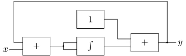
Consider the circuit represented on figure 2.1.1.

+ q R

x +

1

q y Figure 2.1.1: A circuit that admits two distinct solutions as outputs.

The output that we will analyze is the output of the adder at the bottom that we will call y. Similarly to the examples analyzed in the previous chapter, it is not difficult to see that y at time t is given by

4_{In our notation, 0 ∈ N.}

5_{We suppose that the original initial conditions yield unique outputs.}

6_{This is partially true. Although this happens for several important algorithms, there are}

exceptions such as the finite difference methods for solving ODEs [Atk89]. In these methods approximate values are obtained for the solution at a set of grid points

x0< x1< ... < xn< ...

and the approximate value at each xn is obtained by using some of the values obtained in

previous steps. Because we are considering a discrete set of points, an error is introduced in the approximations even if we work with exact numbers. However, if we solve an ODE with a GPAC the same does not happen because we do not use these methods. This is an advantage towards standard numerical methods.

(27)

2.1 Problems of the GPAC

y(t) = 1 + Z _t

0

(y(x) + x)d(y(x) + x).

We are supposing that t0= 0 and that the initial output of the integrator is 0.

When we start the computation, we get two possible solutions: y± = λt.1 ± √ −2t − t. In fact, 1 + Z t 0 (y±(x) + x)d(y±(x) + x) = = 1 + Z t 0 (1 ±√−2x − x + x)d(1 ±√−2x − x + x) = = 1 ±√−2t − t.

Note that y0 _{is not defined for the initial value (t}

0= 0), being one of the reasons

allowing the two solutions. So, we have a non-deterministic circuit.7

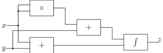
From the mathematical point of view, this seems not to be problematic. The circuit is a specification of the functions generated. Namely, it may be seen as a way to represent graphically a system of ODEs. But we have no reason to assume neither the existence nor the uniqueness of solutions for this system.

The non-determinism of a GPAC is problematic when we take the physi-cal point of view. If we implement the circuit indicated above in a differential analyzer, what would happen? The circuit will only be able to output one solution, so which solution will be picked up, if any? We do believe that the non-determinism will be eradicated when we subject the above differential ana-lyzer not only to the conditions indicated in figure 2.1.1, but also to the known physical laws. In fact, when we deal, for example, with interconnected shafts, there are situations where they can all be blocked up. This situation is not taken in account in the GPAC (as an idealization of mechanical differential an-alyzers). Hence, we believe that if we implement the circuit of figure 2.1.1 in a mechanical differential analyzer, the resulting output will be 1 because we will be unable to turn the input shaft (it will be blocked up). We will be naturally concerned in filtering this kind of behavior.

Another situation not referred above is presented in figure 2.1.2. The inputs are x, y, with x(t0) = y(t0) = 0. We also take the output of the integrator to

be 0 at t = t0. We may take, without loss of generality, t0= 0 (simply compose

the functions defining x and y with t − t0). Suppose that the computation runs

for values of time between 0 and 1. Suppose also that x(1) = y(1) = 1. Then, when the computation is over, we have

z(1) = Z 1

0

¡

x(t)2_{+ y(t)}¢_{d(x(t) + y(t)).}

(28)

GPAC Circuits

Now, if we apply the functions ϕ1= λt.t and ϕ2= λt.t2to the inputs x and y,

respectively, during the interval of time [0, 1], we get z(1) = Z 1 0 (t2_{+ t}2_{)dt +} Z 1 0 (t2_{+ t}2_{)2tdt =} = 5 3.

On the other side, if we now apply ϕ1to y and ϕ2 to x, we get

z(1) = Z 1 0 (t4_{+ t)d(t}2_{+ t) =} 17 10. But 5 3 6=1710!

So, in this circuit, a path dependent behavior occurred: the value of an output depends not only on the present values of the inputs, but also on the path followed by them. So, if we take several inputs in a GPAC, the approaches of taking them as independent variables, or taking them as functions of time are different. Here, we cannot say that z = λxy.z(x, y).

y + x × q q + q R _z

Figure 2.1.2: A circuit with a path dependent behavior.

We also see that in the previous case it is more correct to say that “z is computable by the circuit of figure 2.1.2, relatively to the functions ϕ1and ϕ2”

(or ϕ2 and ϕ1, depending on the situation).

2.2 FF-GPAC Circuits

In this section we will introduce a new model inspired by the GPAC. This model has many desirable properties and permits us to tackle questions raised on the previous section.

We had occasion to see that the output of a unit in a GPAC can be non-unique. We believe that this is due to the lack of restrictions of the GPAC, that allows connections with arbitrarily feedback. As we have observed, feedback is desirable since, without it, we could get an uninteresting model. However, we believe that too much feedback can be harmful.8 _{So, in this new model, we will}

restrict the kind of feedback allowed.

(29)

2.2 FF-GPAC Circuits

Let us first give a brief overview of the standard procedure used to deal with the GPAC (with one independent variable x). As we have already noticed in remark 1.1.2, we can remove multipliers from the definition of the GPAC. So, every GPAC can be built only with adders, constant multipliers, constant function units, and integrators. We can also consider that every output of a GPAC is the output of an integrator (see remark 1.1.1 on p. 8). Proceeding in a similar way as in [Sha41] (or [Pou74]), let U be a GPAC with n − 1 integrators U2, ..., Un, having as outputs y2, ..., yn, respectively. Let y0 = λx.1 and let

y1 = λx.x. Then, each input of an integrator must be the output of one of

the following: an adder, an integrator, a constant function unit, or a constant multiplier. Hence, the integrand of Uk can be expressed as

Pn

i=0c∗kiyi and the

variable of integration asPn_i=0c∗∗

kiyi, for some suitable constants c∗ki, c∗∗ki. Thus,

the output of Uk, yk, can be expressed as

yk = Z _x x0 n X i=0 c∗kiyid  Xn j=0 c∗∗kjyj   + ck, or yk = Z _x x0 n X i,j=0 c∗ kic∗∗kjyidyj+ ck.

We may simplify the last expression by taking ck

ij = c∗kic∗∗kj. It follows that y0 k= n X i,j=0 ck ijyidyj, k = 2, ..., n. (2.1)

In this way we get a system of the form (1.1) (p. 13). Hence, we could assert that it is equivalent to say that y is generated by a GPAC (in the sense that it is a solution for a system of equations where each equation is associated to a unit) and that y is a solution of some system of differential equations with the particular structure of (2.1). Although this seems a clear and natural procedure, we believe that we have to be more careful with it. For instance, why should we consider that an input of the integrator Uk could be expressed as

P_n

i=0ckiyi

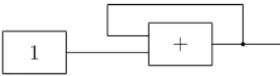
for some constants cki? We could have as input the output of a circuit like

+

1 q

Figure 2.2.1: A circuit that admits no solutions as outputs.

This circuit follows the definition of a GPAC, but we cannot say that its output is a linear combination of the input, because it does not exist. But we would like to keep relations as (2.1). To do so, we will introduce the concept of linear circuit as follows.

Definition 2.2.1 A linear circuit is a GPAC built only with adders, constant multipliers, and constant function units in the following inductive way:

(30)

GPAC Circuits

1. A constant function unit is a linear circuit with zero inputs and one output; 2. A constant multiplier is a linear circuit with one input and one output; 3. An adder is a linear circuit with two inputs and one output;

4. If A is a linear circuit and if we connect the output of A to a constant multiplier, the resulting GPAC is a linear circuit. It has as inputs the inputs of A and as outputs, the output of the constant multiplier;

5. If A and B are linear circuits and if we connect the outputs of A and B to an adder, then the resulting circuit is a linear circuit in which the inputs are the inputs of A and B, and the output is the output of the adder. The proof of the following proposition will be left as an exercise to the reader. Theorem 2.2.2 If x1, ..., xn are the inputs of a linear circuit, then the output

of the circuit will be y = c0+c1x1+...+cnxn, where c0, c1, ..., cn are appropriate

constants. Reciprocally, if y = c0+c1x1+...+cnxn, then there is a linear circuit

with inputs x1, ..., xn and output y.

We next introduce a new type of unit that will be necessary on what follows.9

• Input unit : A zero-input, one-output unit.

The input units may be considered as interface units for the inputs from outside world in order that they can be used by a GPAC (although we may pick an output directly from the GPAC).

We now present the main definition of this section.

Definition 2.2.3 Consider a GPAC U with n integrators U1, ..., Un. Suppose

that to each integrator Ui, i = 1, ..., n, we can associate two linear circuits,

Ai and Bi, with the property that the integrand and the variable of integration

inputs of Ui are connected to the outputs of Ai and Bi, respectively. Suppose

also that each input of the linear circuits Ai and Bi is connected to one of

the following: the output of an integrator or to an input unit. U is said to be a feedforward GPAC (FF-GPAC) iff there exists an enumeration of the integrators of U, U1, ..., Un, such that the variable of integration of the kth integrator can be

expressed as ck+ m X j=1 ckjxj+ k−1_X i=1 ¯ckiyi, for all k = 1, ..., n, (2.2)

(see fig. 2.2.2) where yi is the output of Ui, for i = 1, ..., n, xj is the input

associated to the jth input unit, and ck, ckj, ¯cki are suitable constants, for all

k = 1, ..., n, j = 1, ..., m, and i = 1, ..., k − 1.

9_{These units correspond to the elements of X introduced in the definition given on the}

(31)

2.2 FF-GPAC Circuits

Remark 2.2.4 In a FF-GPAC we can link the output of Uk directly to the

input of Ur (as long as (2.2) is satisfied) because this is equivalent to have a

constant multiplier associated to the value 1 between them.

We can also have a notion of function generated by a FF-GPAC using a straightforward adaptation of the homonymous definition for the case of the GPAC (see p. 6). We can also suppose that each function generated by a FF-GPAC is the output of an integrator (see remark 1.1.1).

Remark 2.2.5 When considering an enumeration U1, ..., Un of integrators of a

FF-GPAC U, we will always assume that it satisfies condition (2.2). R

L(1,x1,...,xm,y1,...,yk−1)

L(1,x1,...,xm,y1,...,yn) _y k

Figure 2.2.2: Schema of the inputs and outputs of Uk in the

FF-GPAC U. L(z1, ..., zr) denotes a linear combination (with

real coefficients) of z1, ..., zr.

As examples of FF-GPACs we have all the circuits presented in section 1.2. For the circuits of figures 1.2.1 and 1.2.2, we can take enumerations of integrators starting from the right and going to the left to see that they are FF-GPACs.10

A similar argument applies to the circuit of figure 1.2.3.

It is clear that if a unary function y is generated by a FF-GPAC, it is generated by a GPAC (because each FF-GPAC is a GPAC) and it satisfies some system of equations with structure similar to (2.1). The converse relation does not hold. Take, for example, the GPAC represented in figure 2.1.1. Applying the standard procedure for a GPAC (see p. 21), we conclude that every output of the circuit will satisfy some system of differential equations similar to (2.1). But this circuit is not a FF-GPAC. We will see that the subclass of the GPAC constituted by FF-GPACs still preserves the desirable properties of the T-GPAC.

Remark 2.2.6 If we consider a FF-GPAC U with n integrators U1, ..., Un,

cor-responding to the outputs z1, ..., zn, respectively, and having inputs x1, ..., xm,

we define y0, ..., yn+mby yi=    λx.1 if i = 0, xi if 1 ≤ i ≤ m, zi−m if m < i ≤ m + n.

Then (2.2) can be written as

k−1

X

i=0

ckiyi, for all k = m + 1, ..., m + n,

for suitable constants cki.

10_{In a FF-GPAC, we do not take multiplier units. However, a circuit like the one of figure}

(32)

GPAC Circuits

Before continuing with our work, we have to set up more conditions on this model. We have admitted that the inputs x1, ..., xmof a GPAC are functions of

a parameter t. But we didn’t make any assumption on these functions (about computability, smoothness, or whatever). When we consider the integrator units, one problem still arises: if I = [a, b] is a closed interval, the Riemann-Stieljes integralR_Iϕ(t)dψ(t) is not defined for every pair of functions ϕ, ψ, even if they are continuous.

It is possible to show [Str99, pp. 7,9] that it suffices to consider that ψ is continuously differentiable on I. Then

Z I ϕ(x)dψ(x) = Z I ϕ(x)ψ0_(x)dx, and _¯ ¯ ¯ ¯ Z I ϕ(x)dψ(x) ¯ ¯ ¯ ¯ ≤ Kψkϕk∞,

where Kψ = kψ0k_∞(b − a). So, from now on, we will always assume that the

inputs are continuously differentiable functions of the time. And if the outputs of all units are defined for all t ∈ I, where I is an interval, then we will also assume that they are continuous in that interval.11 _{This is needed for the}

following results and may be seen as physical constraints to which all units are subjected.

2.3 Basic Properties

In this section we show that some of the problems referred on section 2.1 can be solved for the FF-GPAC. We first prove a theorem that guarantees that if the inputs are of class Cr_{, r ≥ 1, then the outputs are also of class C}r_.

Theorem 2.3.1 Suppose that the input functions of a FF-GPAC are of class Cr _{on some interval I, for some r ≥ 1, possibly ∞. Then the outputs are also}

of class Cr _{on I.}

Proof. Suppose that we have a FF-GPAC U with m inputs and n integrators. To show our result we only have to prove that the output of every integrator is of class Cr_{. We will first show the result for r < ∞ using induction on r. We}

use the notation indicated in remark 2.2.6. Then yk= Z t t0 Ã_n+m X i=0 c∗ kiyi ! d   k−1 X j=0 c∗∗ kjyj   + ck, k > m,

11_{It is not a difficult task to show that this condition can be replaced by the following: if I}

is closed and if y is the output of an integrator, then there exists some L > 0 such that, for

(33)

2.3 Basic Properties

where c∗

ki, c∗∗kj, ck, for i = 0, 1, ..., n+m, k = m+1, ..., n+m, and j = 0, 1, ..., k−1,

are suitable constants. We begin with r = 1. Then ym+1= Z _t t0   n+m_X i=0 m X j=1 c∗m+1ic∗∗m+1jyiyj0  dt + cm+1. Let ck

ij = c∗kic∗∗kj. The integrand part is continuous and we can therefore apply

the Fundamental Theorem of Calculus to conclude that ym+1 is differentiable

and that y0 m+1= n+m_X i=0 m X j=1 cm+1_ij yiy0j.

So, ym+1is of class C1. Now suppose that the result is true for all k such that

m < k < p, for some p ≤ n + m. Then, by similar arguments, we can show that yp is differentiable and that

y0 p= n+m_X i=0 p−1 X j=1 cp_ijyiyj0.

Therefore, ym+1, ..., ym+n are all of class C1. Now suppose that r > 1. If the

inputs x1, ..., xm are of class Cr, then they are also Cr−1 functions. So, by

induction hypothesis, ym+1, ..., ym+n are all of class Cr−1. We now show that

ym+1is a function of class Cr. We already know that ym+1is differentiable and

that ym+10 = n+m_X i=0 m X j=1 cm+1_ij yiy0j.

But all the functions at the right side are of class Cr−1_{. So, we can differentiate}

the right expression r − 1 times obtaining a continuous function. Then ym+1is

of class Cr_{. A similar argument shows that the functions y}

m+1, ..., ym+nare all

of class Cr_{. Finally, if r = ∞, then all the derivatives of y}

m+1, ..., ym+n exist

and, hence, these functions are of class C∞_.

Next we will focus to the problem of existence and uniqueness of outputs. We will need the following theorem (theorem 6.11 of [BR89]).

Theorem 2.3.2 Let f (x, t) be defined and of class C1 _{in an open region R of}

Rn+1_{. For any (c, a) in the region R, the differential equation}

x0_{(t) = f (x, t)}

has a unique solution x(t) satisfying the initial condition x(a) = c and defined for an interval a ≤ t < b (where b may eventually be ∞) such that, if b < ∞, either x(t) approaches the boundary of the region, or x(t) is unbounded as t → b.

(34)

GPAC Circuits

Remark 2.3.3 If we apply the previous theorem to the function g = λxt.f (x, −t) and the theorem 6.8 of [BR89], we can prove a similar result, but for an interval (b0, b1), where b0, b1 are constants such that b0< a < b1.

Next, we show a theorem that guarantees the existence and the uniqueness of outputs for FF-GPACs with only one input.

Theorem 2.3.4 Suppose that we have a FF-GPAC with only one input x, of class C1_{on an interval [t}

0, tf), where tf may possibly be ∞. Then there exists

an interval [t0, t∗) (with t∗≤ tf) where each output exists and is unique.

More-over, if t∗ _{< t}

f, then there exists an integrator with output y such that y(t) is

unbounded as t → t∗_.

Proof. Suppose that we have a FF-GPAC U with n − 1 integrators. Using the notation of theorem 2.3.1 and proceeding in a similar way, we conclude that

y0 k= n X i=0 k−1 X j=1 ck ijyiyj0, k = 2, ..., n, where ck

ij are suitable constants. We can write this as

y0 k− k−1 X j=2 Ã _n X i=0 ck ijyi ! y0 j= n X i=0 ck i1yi, k = 2, ..., n.

This system may be written in the following way      1 0 · · · 0 −Pn_i=0c3 i2yi 1 · · · 0 .. . ... . .. ... −Pn_i=0cn i2yi − Pn i=0cni3yi · · · 1           y0 2 y0 3 .. . y0 n     =      Pn i=0c2i1yi Pn i=0c3i1yi .. . Pn i=0cni1yi      or simply Ay0 = b, where y =    y2 .. . yn    .

It is easily seen that det A = 1. Hence A is invertible and we have A−1 = 1

det AAcof,

where Acof is the transpose of the matrix in which each entry is its respective

cofactor with respect to A (cf. [Str88]). So, each entry in A−1 _{is a polynomial}

in x, y2, ..., yn. The same happens for b. We know that

y0_{= A}−1_b.

Then we may write

(35)

2.3 Basic Properties

where each component of p is a polynomial in x, y2, ..., yn, defined on all Rn+1.

Hence, by remark 2.3.3, if x(t0) = x0, then there exists an interval (a, b), with

a < x0< b, where the solution of the previous system associated to the initial

condition y(x0) = y0exists and is unique. Hence, because R = Rn+1, we have

b = ∞ or y(x) is unbounded as x → b. A similar result holds for a. Let

A0= {t ∈ [t0, tf) : a < x(t) < b}.

Because we assumed that the inputs were continuous functions of the time and that (a, b) is an open set, we conclude that A0 is also open (in order to the

subspace topology of [t0, tf). For the topological results indicated here, refer to

[Mun00, Lip65]). But [t0, tf) is locally connected and, hence, each component

of A0 is open on [t0, tf) (theorem 25.3 from [Mun00]). Let A be the component

of A0such that t0∈ A. A must be open. Hence A = [t0, t∗), where t∗is possibly

tf. If t∗ < tf then, because t∗ ∈ A and A is a component, we conclude that/

x(t∗_{) /}_{∈ (a, b). But if {t}

n}n∈N is a sequence in A that converges to t∗, then

x(tn) ∈ (a, b). Because x is continuous, it must be x(t∗) = a or x(t∗) = b. So,

when {tn}n∈Nis a sequence in A that converges to t∗(and t∗< ∞), we conclude

that x(tn) converges to a or to b. Suppose, without loss of generality, that it

converges to b. Then b < ∞ because x(t) is defined for t ∈ [t0, tf) and b = x(t∗),

with t∗_{∈ [t}

0, tf). But if b < ∞, then y(x) is unbounded as x → b. Hence, from

lim

n→∞x(tn) = b

we conclude that y(tn) ≡ y(x(tn))) is unbounded as tn→ t∗.

The previous result applied only to FF-GPACs with one input. Next we present a slightly weaker result for FF-GPACs with more than one input. Theorem 2.3.5 Consider a FF-GPAC with m inputs x1, ..., xmof class C2 on

an interval [t0, tf), where tf may possibly be ∞. Then there exists an interval

[t0, t∗) (with t∗≤ tf) where each output exists and is unique. Moreover, if t∗< tf

then there exists an integrator with output y such that y is unbounded as t → t∗_.

Proof. Suppose that we have a FF-GPAC U with n integrators U1, ..., Un, with

outputs y1, ..., yn, respectively. Then, for k = 1, ..., n, we have

yk = Z t t0   m X i=0 c∗ kixi+ n X j=1 ckjyj  d Ã_m X r=0 b∗ krxr+ k−1 X s=1 bksys ! + ck, where c∗

ki, ckj, b∗kr, bks, ck are real constants. Let

ϕk= m X i=0 c∗kixi, ψk= m X r=0 b∗krxr, k = 1, ..., n.

By the Fundamental Theorem of Calculus, we get y0 k =  ϕk+ n X j=1 ckjyj   Ã ψ0 k+ k−1 X s=1 bksy0s ! ,

(36)

GPAC Circuits

for k = 1, ..., n. Rewriting the last expression, we obtain y0 k− k−1 X s=1  ϕk+ n X j=1 ckjyj   bskys0 =  ϕk+ n X j=1 ckjyj   ψ0 k (2.3) for k = 1, ..., n. Let A =        1 0 · · · 0 −³ϕ2+ P_n j=1c2jyj ´ b12 1 · · · 0 .. . ... . .. ... −³ϕn+ P_n j=1cnjyj ´ b1n − ³ ϕn+ P_n j=1cnjyj ´ b2n · · · 1        and b =      ³ ϕ1+ P_n j=1c1jyj ´ ψ0 1 .. . ³ ϕn+ Pn j=1cnjyj ´ ψ0 n     . Then, the system (2.3) may be written as

Ay0 _{= b.}

Note that, because x1, ..., xm, y1, ..., ynare C2-functions, each component of b is

continuously differentiable (in order to t) and each element of A is of class C2_.

We also have det(A) = 1. Hence A is invertible and each entry of A−1 _{can be}

obtained from x1, ..., xm, y1, ..., ynusing only products and additions (remember

that ϕk and ψk, k = 1, ..., n, are obtained in this way). Then each component

of A−1 _{is of class C}2 _and

y0_{= A}−1_{b = f ,}

where each component of f is continuously differentiable. Now we could apply theorem 2.3.2 to conclude the result. But one condition fails: the domain of f , [t0, tf), is not open. Nevertheless, if we extended the inputs x1, ..., xn to

the interval (−∞, tf), maintaining the condition of being twice differentially

continuous, we have our problem solved. Therefore we only have to extend the inputs. We may do this by picking

¯ xk= λt.

½

c0+ c1(t − t0) + c2(t − t0)2, if t ∈ (−∞, t0),

xk, if t ∈ [t0, tf),

for k = 1, ..., m, where c0 = xk(t0), c1 = x0k(t0), and c2 = x

00 k(t0)

2 . It is a trivial

exercise to verify that ¯xk ∈ C2((−∞, tf)) for k = 1, ..., m.

The previous theorems applied on an interval of time [t0, tf), where t0 is the

initial value. This correspond to the physical notion of time, where we cannot, in principle, go back in time (irreversible systems). But as we already referred,