The Presence of Distortions in the Extended Skew-normal Distribution
Antonio Seijas-Macias*Universidade da Coruña and Universidad Nacional de Educación a Distancia (UNED), A Coruña, Spain – [email protected]
Amílcar Oliveira
Universidade Aberta and Centro de Estatística e Aplicações, Faculdade de Ciências, Universidade de Lisboa, 1749-016 Lisboa, Portugal. – [email protected]
Teresa Oliveira
Universidade Aberta and Centro de Estatística e Aplicações, Faculdade de Ciências, Universidade de Lisboa, 1749-016 Lisboa, Portugal – [email protected]
Abstract
In the last years, a very interesting topic has arisen and became the research focus not only for many mathematicians and statisticians, as well as for all those interested in modeling issues: The Skew normal distributions’ family that represents a generalization of normal distribution. The first generalization was developed by Azzalini in 1985, which produces the skew-normal distribution, and introduces the existence of skewness into the normal distribution. Later on, the extended skew-normal distribution is defined as a generalization of skew-normal distribution. These distributions are potentially useful for the data that presenting high values of skewness and kurtosis. Applications of this type of distributions are very common in model of economic data, especially when asymmetric models are underlying the data. Definition of this type of distribution is based in four parameters: location, scale, shape and truncation. In this paper, we analyze the evolution of skewness and kurtosis of extended skew-normal distribution as a function of two parameters (shape and truncation). We focus in the value of kurtosis and skewness and the existence of a range of values where tiny modification of the parameters produces large oscillations in the values. The analysis shows that skewness and kurtosis present an instability development for greater values of truncation. Moreover, some values of kurtosis could be erroneous. Packages implemented in software R confirm the existence of a range where value of kurtosis presents a random evolution.
Keywords: Skewness; Kurtosis; Skew normal; Computational Cumulants.
JEL Classification: C15, C63
1. Introduction
The skew-normal probability distribution (Azzalini, 1985) was introduced by Azzalini in 1985 which including the normal distribution as a special case. The skew-normal is a generalization of the normal distribution where the more important characteristic is the presence of different level of skewness. In the motivation of this new approach to the normal distribution there are two basic: first motivation, lies in the essence of the mechanism which starts with a continuous symmetric density function that then is modified to generate a variety of alternative forms (Azzalini & Capitanio, 2014, page 1). The second one is the need to approximate the real data with the theoretical distributions using the fewer unrealistic assumptions for the model.
In the seminal paper (Azzalini, 1985), author considers a generalization of the skew-normal distribution that is named as extended skew-normal distribution, which skew-normal one is an instance. Generalization to the bivariate case and multivariate one are analyzed in Arnold et al. (1993) and Capitanio et al. (2003).
The skew-normal is derived from the standard normal density function ϕ and the standard normal distribution function Φ. In the univariate case the skew-normal a random variable X is distributed as a skew-normal distribution with density function
fX(x) = 2 ωϕ ( x − ξ ω ) Φ (α x − ξ ω ).
where we use three parameters: location ξ ∈ ℝ, scale ω ∈ ℝ+ and shape α ∈ ℝ. When ξ = 0 and ω = 1 then we have the normalized skew-normal distribution, and the only free parameter α determines the skewness level. As a special case for α = 0 then we have the standard normal distribution N (0,1) with skewness equals zero and kurtosis equals 3. Obviously, the parameter α could control the skewness of the distribution. Unfortunately, kurtosis is not considered.
The introduction of a new parameter τ ∈ ℝ, named truncation parameter produces the extended skew-normal distribution. For the univariate case, the density function for the Extended Skew-Normal distribution (ESN) is fX(x) = 1 ωϕ ( x − ξ ω ) Φ (τ√α2+ 1 + αx − ξ ω ) Φ(τ) .
For the case, which α = 0 then we have the skew-normal distribution and ω = 0 the normal one. In Canale (2011) some properties of the density function are presented and the name of truncation for the new parameter τ is explained. The effect of the new parameter τ has consequences on the skewness and the kurtosis of the distribution of the random variable. The effect of the τ is not independent of the parameter α. For the smaller value of α variations on τ it produces less effect on the shape of the distribution. Basically, the two parameters determine values of skewness and kurtosis of the distribution. During last years, the use of Skew-normal distribution and ESN is increasing, to represent different types of data with skewness and where the test of normality (Shapiro Test) is not satisfied (Canale, 2011). Some authors (Figueiredo & Gomes, 2013; Chenglong et al. 2017) consider different types of hypothesis contrast using the Skew-normal and ESN distributions.
For R software (2015) the package sn, developed by Azzalini, provides facilities to define and manipulate probability distributions of the skew-normal family and some related ones. The first version of the package was written in 1997, and in 2014 the version 1.0-0 was uploaded to CRAN. In this paper, we have used the implemented functions available in the version 1.4-0 of the package.
2. Skewness and Kurtosis of ESN
The moment generating function of an ESN distribution is computed from the expression Y = ξ + ωZ where Z ∼ SN(0,1, α, τ), as in M(t) = exp (ξt +1 2ω 2t2)Φ(τ + δωt) Φ(τ) where δ = α √1+α2.
Expressions for the statistics (mean, variance, skewness and kurtosis) could be calculated as a function of the derivatives of the moment-generating function. Skewness and kurtosis are independent of the values of the two first parameters of extended skew-normal distribution; only α and τ are relevant. The value of mean and variance is a function of the four parameters.
Another approach is using the cumulant generating function given by: κ(t) = logM(t) = ξt +1
2ω
2t2+ ζ
0(τ + δωt) − ζ0(τ)
where ζ0(x) = log2Φ(x) and ζr(x) = drζ0(x)
dxr , with r = 1,2, . ... The derivatives of κ(t) are κi, the cumulant of order i. Thus, the derivatives of ζ are:
1. ζ1(x) = dζ0(x) dx = exp(log(ϕ(x)) − log(Φ(x))) 2. ζ2(x) = −ζ1(x)(ζ1(x) + x) 3. ζ3(x) = −ζ2(x)(ζ1(x) + x) − 2ζ2(x)(1 + ζ2(x)) = ζ1(x)(ζ1(x) + x)2− ζ1(x)(1 − ζ1(x)(ζ1(x) + x)) 4. ζ4(x) = −ζ3(x)(2ζ1(x) + x) − 2ζ2x(1 + ζ2(x)) = −(ζ1(x)(ζ1(x) + x)2− ζ1(x)(1 − ζ1(x)(ζ1(x) + x))) ∗ (x + 2ζ1(x)) + 2ζ1(x)(ζ1(x) + x)(1 − ζ1(x)(ζ1(x) + x))
The values of mean, variance, skewness and kurtosis are calculated from the cumulants: 1. Cumulant of first order is the mean.
2. Cumulant of second order is the variance. 3. Skewness is calculated as κ3 κ23/2= ζ3(τ)δ3 (1+ζ2(τ)δ2)(3/2). 4. Kurtosis is calculated1 as κ4 κ22+ 3 = ζ4(τ)δ4 (1+ζ2(τ)δ2)2+ 3.
Value of cumulants is obtained by function sn.cumulants(ψ, ω, α, τ, n) where n is the number of cumulants (default=4, max=6). This procedure is part of the package sn (Azzalini, 2004).
The value of mean and variance are directly, but for calculation of the skewness and kurtosis could be obtained using the cumulants of order 3 and 4, respectively and the cumulant of order 2. For example: Considering the extended skew normal with parameters ξ = 0, ω = 1, α = −50, τ = −6, skewness is −1.825792 and kurtosis is 4.874607. Mean and variance of ESN(0,1,-50,-6) is given by the two first elements of the result of procedure sn. cumulants, then, mean equals −6.157251 and variance is 0.0243778.
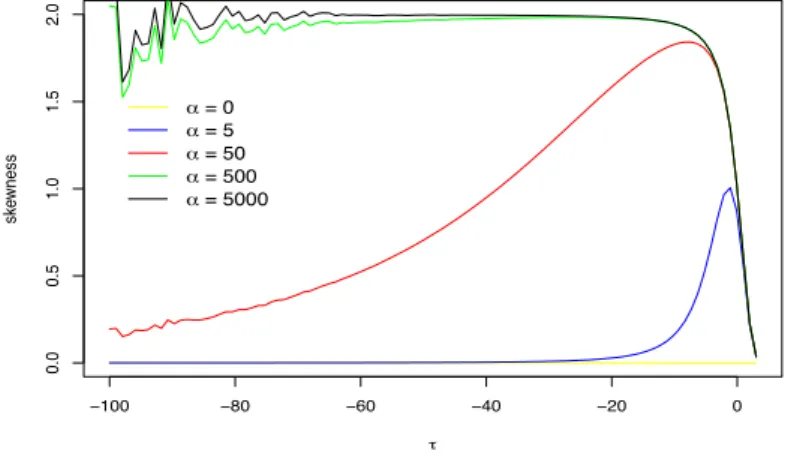
Figure 1: Evolution of skewness ESN distribution for several values of 𝛼.
The sign of α determines the sign of skewness, when α < 0 then skewness is negative and α > 0 is associated to positive skewness. For α = 0 then skewness is 0. The value of τ determines the value of skewness that tends to zero when τ → ±∞, although is more sensible for the positive branch. Figure 1 shows the evolution of skewness for several values of α as a function of τ. Range of skewness is in (−2,2).
For positive values of τ skewness tend to zero when τ is increasing, for smaller values; but in the negative branch skewness presents a wider range of variation, although, when τ decrease, skewness decreases to zero (for positive values of α) and skewness increases to zero (for negative values of α). In Canale (2011), the maximum value of skewness is cited as 1.995, but the observation of the figure 1 shows, for values of τ negative and very large the presence of oscillations that produce values of kurtosis greater than 2. We might consider that situations as errors for the precision machine limits of computers. As consequence, the level of skewness is around 2 and no decreasing movement to zero is observed. The approach for lower values of τ reduce the range for skewness to interval (−2,2), but using the
sn.cumulants function some strange values for skewness are possible, when α is greater (more than
1000) and τ < −500, in this case the range of values of skewness is increasing when τ is decreasing.
1Some authors consider the excess kurtosis that is the quotient between cumulant of order 4 and the square of
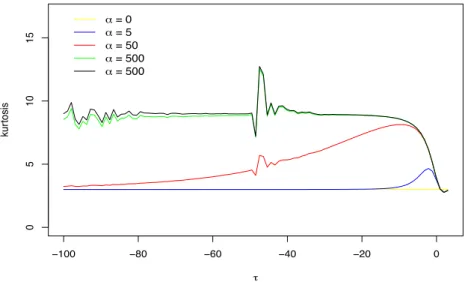
Kurtosis presents the same strange oscillations for greater values of α and when τ is large and negative (see figure 2). But now, the oscillations appear for lower values (t ≤ −40).
Figure 2: Evolution of kurtosis ESN distribution for several values of 𝛼.
The range of kurtosis of the ESN distribution could be (2,10). The large value of 𝛼 the large value of kurtosis (although a limit could be exists rounded 10). And when |𝜏| is large, kurtosis tends to zero. This tendency is more sensitive in the positive side. For very large values of 𝛼 (> 50) kurtosis tends to 10 but oscillations produce values very large > 15.
In Azzalini & Capitanio (2014), Fig. 2.5 shows graphically the range of skewness and kurtosis (excess kurtosis) with the Extended Skew-normal distribution with 𝛼 > 0 and 𝜏 ∈ (−10, 2). The range of both statistics is wider than in the Skew-normal distribution, but the whole range is limited. However, there is no reference to the oscillations of skewness and kurtosis that appears when values for 𝜏 < −50 and 𝛼 > 500 are considered.
3. Oscillations in Skewness and Kurtosis of the ESN Distribution.
A graphical analysis of the evolution of the values of both statistics for α > 500 and τ < −50 showed the presence of instabilities and oscillations on the range of the values. In this section, we analyses the reasons for that will be studied.
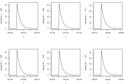
Shape of the density function (PDF) of the ESN distribution might be affected by the oscillations into skewness and kurtosis. But we can prove, using an example, that the shape of function doesn’t reflect the variations of those statistics, see Figure 3.
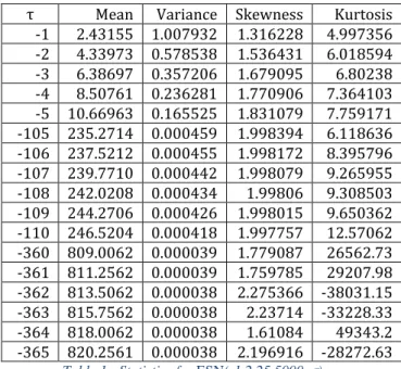
The evolution of the shape of the density function is very smooth. In figure 3, it can be observed the pdf of several ESN distributions for ξ = −1, ω = 2.25, α = 5000 and τ = [−110, −105]. The same effect is observed for large values of the parameter τ (Figures 4), in this case the shape of the distribution is the same for values τ = {−360, −361, −362, −363, −364, −365}. One can conclude that oscillations in skewness and kurtosis are not reflected at the shape of the distribution which presents a regular evolution without deep variations.
Figure 3: PDF of 𝐸𝑆𝑁(−1,2.25,5000, 𝜏)𝜏 ∈ [−110, −105]
Figure 4: PDF of 𝐸𝑆𝑁(−1,2.25,5000, 𝜏) 𝜏 ∈ [−365, −360]
The statistics are in table 1. Skewness and kurtosis are increasing as τ is increasing, but the variation is decreasing, in a concave manner; however, when the value of τ is large and negative, the evolution of both statistics is strange and it presents oscillations.
When considering the more negative values for τ and large values for α, the skewness and kurtosis has strange oscillations for small variations. Theses variations could not be reflected at the shape of the pdf of the Extended Skew-normal distribution.
235.20 235.30 235.40 0 1 0 2 0 3 0 4 0 x d e n s it y f o r t = -1 0 5 237.45 237.55 237.65 0 1 0 2 0 3 0 4 0 x d e n s it y f o r t = -1 0 6 239.70 239.80 239.90 0 1 0 2 0 3 0 4 0 x d e n s it y f o r t = -1 0 7 241.95 242.05 242.15 0 1 0 2 0 3 0 4 0 x d e n s it y f o r t = -1 0 8 244.20 244.30 244.40 0 1 0 2 0 3 0 4 0 x d e n s it y f o r t = -1 0 9 246.45 246.55 246.65 0 1 0 2 0 3 0 4 0 x d e n s it y f o r t = -1 1 0 808.96 809.00 809.04 0 2 0 4 0 6 0 8 0 1 2 0 x d e n s it y f o r t = -3 6 0 811.20 811.24 811.28 0 2 0 4 0 6 0 8 0 1 2 0 x d e n s it y f o r t = -3 6 1 813.46 813.50 813.54 0 2 0 4 0 6 0 8 0 1 2 0 x d e n s it y f o r t = -3 6 2 815.70 815.74 815.78 0 2 0 4 0 6 0 8 0 1 2 0 x d e n s it y f o r t = -3 6 3 817.96 818.00 818.04 0 2 0 4 0 6 0 8 0 1 2 0 x d e n s it y f o r t = -3 6 4 820.20 820.24 820.28 0 2 0 4 0 6 0 8 0 1 2 0 x d e n s it y f o r t = -3 6 5
τ Mean Variance Skewness Kurtosis -1 2.43155 1.007932 1.316228 4.997356 -2 4.33973 0.578538 1.536431 6.018594 -3 6.38697 0.357206 1.679095 6.80238 -4 8.50761 0.236281 1.770906 7.364103 -5 10.66963 0.165525 1.831079 7.759171 -105 235.2714 0.000459 1.998394 6.118636 -106 237.5212 0.000455 1.998172 8.395796 -107 239.7710 0.000442 1.998079 9.265955 -108 242.0208 0.000434 1.99806 9.308503 -109 244.2706 0.000426 1.998015 9.650362 -110 246.5204 0.000418 1.997757 12.57062 -360 809.0062 0.000039 1.779087 26562.73 -361 811.2562 0.000039 1.759785 29207.98 -362 813.5062 0.000038 2.275366 -38031.15 -363 815.7562 0.000038 2.23714 -33228.33 -364 818.0062 0.000038 1.61084 49343.2 -365 820.2561 0.000038 2.196916 -28272.63
Table 1: Statistics for ESN(-1,2.25,5000, 𝜏)
For studying, the reasons for oscillations into the values of kurtosis and skewness, we must analyses the cumulants. Skewness is a function of δ that depends only of the parameter α, the range δ ∈ (−1,1), thus when α → ∞ then δ → 1 and α → −∞ then δ → −1 and δ = 0 when α = 0. The other elements in skewness are ζ2(τ) and ζ3(τ), both of them are functions of ζ1 that is the first derivative of ζ0(x) =
log2Φ(x) without analytical expression for τ ∈ (−∞, ∞). For values of τ < −50 an expression using a series expansion.
Figure 5: Evolution of 𝜁2(𝜏), 𝜁3(𝜏), 𝜁4(𝜏)
For large negative values of τ, ζ1(τ) → −τ and factor τ + ζ1(τ) ∈ (0,0.02) then range ζ2(τ) ∈
(−1, −0.9996), both elements are increasing function of τ. The shape is smooth, but when analyzing the factor ζ3 one can observed that for values of τ < −100 there is oscillations in the value in the range
(−1 ∗ 10−5, 1 ∗ 105), that is probably cause of oscillation in skewness, and are more evident for large
Figure 5). In the graphic one can observed evolution of the components of the skewness (ζ2, ζ3) in the
range (−110, −106) and (−365, −360), in the first case there is not oscillations and the value of skewness is smooth increasing but, in the second case, the oscillations of ζ3 are the explanation of the
movements of the values of skewness, without a defined trend.
Kurtosis is a function of ζ2 and ζ4, and oscillations are more evident because the presence of ζ3 in the
expression of ζ4 produce a wider movement. Oscillations are evident for smaller negative values of τ
(see Figure 5). Oscillations into ζ2, ζ3 and ζ4 are a consequence of the definition of ζ1 that is a nonlinear
function of τ. The difference between two consecutive elements tends to 1 when τ tends to -∞, as the range of variation is very small and the shape of ζ1 is quasi-linear. However, this effect is augmented in
calculation of ζ2, ζ3 and ζ4. Variations in ζ1 and ζ2 preserves the sign, but for large negative values of τ
preservation of sign do not hold for ζ3 and ζ4, and that is the reason for the existence of jumps in
skewness and kurtosis.
4. Conclusions
The Extended Skew-Normal distribution (Azzalini & Capitano, 2014) is developed as a generalization of the normal distribution, considering the existence of skewness. The normal distribution would be a special case of the extended skew-normal with skewness equals zero and kurtosis equals 3 (excess kurtosis null). For the software R, a package for the extended skew-normal distribution is available, named sn. The development of the package is referred in the webpage http://azzalini.stat.unipd.it/SN/. The Extended Skew-Normal distribution is a function of four parameters, where ξ, α, τ ∈ ℝ and ω > 0. Nevertheless, the range of variation of the other parameters is not limited.
In this paper, we have observed that for values of τ < −8 the statistics (skewness and kurtosis) of the distribution present oscillations and, for large negative values of τ and large values of α kurtosis presents no reasonable values.
Effects are different for skewness and kurtosis. Skewness presents a trend to established around 2 but with big oscillations when small variations of τ are considered. Kurtosis presents larger variations with values very large, and, in same cases, the sign is not according the theory of distribution.
Although the sn package is valid for the study of extended skew-normal distribution we might be careful for τ negative values. For τ < −8, the results could not be trustable because the presence of errors in the statistics and distribution could not defined in a well-manner.
Acknowledgement
This work was partially supported by Fundaçao para a Ciência e a Tecnologia, Portugal - FCT [UID/MAT/00006/2013].
References
Azzalini, A. (1985). “A class of distributions which includes the normal ones” in Scandinavian Journal of Statistics, 12, 171-178.
Azzalini, A. & Capitanio. A. (2014). The Skew-Normal and Related Families. Institute of Mathematical Statistics Monographs (IMS). Cambridge University Press.
Canale, A. (2011). “Statistical aspects of the scalar extended skew-normal distributions” in Metron, LXIX (3), 279-295.
Capitanio, A., Azzalini, A. & Stanghellini, E. (2003). “Graphical models for skew-normal variates” in Scandinavian Journal of Statistics, 30, 129-144.
Chenglong, L., Mukherjee, A., Qin, S. & Min, X. (2017) “Some monitoring procedures related to assymetry parameter of azzalini’s skew-normal model” Accepted for publication in Revstat – Statistical Journal.
Figueiredo, F., Gomes, M. (2013). “The skew-normal distribution in spc” in Revstat – Statistical Journal, 11(1), 83-104.
Team, R.C. (2015). A language and environment for statistical computing. R Foundation for Statistical Computing. Vienna.