UNIVERSITY OF BEIRA INTERIOR
Faculty of Engineering
A Platform to Support the Development of
Applications Based on the Segmentation and
Labelling Algorithm
Sabrina Santos Guia
Dissertation to obtain the Master’s Degree in
Electrical and Computer Engineering
(2
ndstudy cycle)
Advisor: Professor Doctor António Eduardo Vitória do Espírito Santo
Co-advisor: Professor Doctor Vincenzo Paciello
and reminding that
“Just because
something doesn’t do
what you planned it
to do doesn’t mean
it’s useless.”
Thomas Alva Edison
“I haven’t failed…
I’ve just found 10,000 ways that won’t work!”
and I learned that
“When you have exhausted all possibilities,
remember this: you haven’t.”
because
“Our greatest weakness lies in giving up!
The most certain way to succeed is always to try
Acknowledgements
To my advisor Professor Doctor António Eduardo Vitória do Espírito Santo and to my co-advisor Professor Doctor Vincenzo Paciello, for their availability to discuss and dispel doubts and uncertainties, for the sincerity and exemplary professionalism that they have shown. For the interest in showing me devices and electronic equipment and teach me new concepts, even though they were not related to the project in development. For encouraging the growth both personally and academically. I am also grateful for the scientific orientation, and for any suggestions made during the writing and development of this project and its final revision. To Tânia Campos and Pedro Serra, for the sympathy and availability and patience in making all the linguistic revision.
To Tuna Feminina da Universidade da Beira Interior – “As Moçoilas”, that beyond the good and bad times past have always supported and helped me. For having entrusted the post of association leader and have inculcated a way of life.
To Patrícia Melo and Fabiana Guilherme, by understanding and friendship that although the distance, always supported me throughout my academic career, always leaving me nostalgic for the moments with the Banda Musical de Gouviães and from Escola EB 2,3/S de Tarouca, respectively.
To Kelly Amaral, Hugo Oliveira, Tiago Mota, Joana Serralheiro, Tiago Ferreira, Marina Barbosa, Filipa Moreira, Elisabete Alves and Valéria Nascimento the endless hours of willingness spent in labour talks, but more importantly by the sincere friendship, support and patience in being with me in the hardest times. For the teachings transmitted not only over the degree in Bioengineering but also throughout the master's degree in Electrical Engineering and Computer in the Bionic Systems Branch.
To my parents for all the sacrifices in giving me always all it took, sometimes more than was possible to them, throughout my academic journey. I am also grateful for the affection and unconditional support, though at distance, were always by my side encouraging to never give up!
Finally, to all those who, indirectly, contributed to this work, in particular, all colleagues and professors from the Universidade da Beira Interior and all members from the MISTRAL Laboratory of the Università Degli Studi di Salerno, my most sincere acknowledgments.
Abstract
The need for networks of sensor that operate in an increasingly efficient way is contributing to boost the research methods with the aiming of find the best methods about how to manage the information. At the same time, the technological explosion that is taking care of our daily life, have influence not only on what is likely to be standardized, but also in the possibility of execution. An example of this is the need to exchange the knowledge about how the sensor’s signal behaves in a standardized manner, as well as, some of its features and isolated parameters. The compaction of data to be managed and transmitted clearly becomes useful, especially when there is interest in the study of signal characteristics, such as; amplitude; the presence of noise; steady state values tendency, etc. Small parameter capable of induce the general behaviour of the measured signal.
In the world of sensors, intelligence is focused on the same point of measurement made by the transducer. From this point, three algorithms are presented. The first is based on the rapid measurement of procedural techniques of the Fourier transform (FFT), while the second is based on the compressive sampling theory (CS). Finally it is presented a proposed algorithm, in the time domain, based on the processes of segmentation and labelling (S&L) of a sampled signal that is also proposed for defining the new IEEE 1451 standard. The main goal of this work is focused on the management of a smaller amount of data, but the acquisition of the same amount and quality of information. Thus, the ideal is that the signal is sampled in order to create redundancy between neighbouring samples. It is therefore not necessary segmentation of each pair of samples, storing and transferring only the samples that are held to bring important information. As a result of the segmentation process, two vectors are obtained for storing amplitudes and time indices of samples and labelling process, the segments are classified according to their behaviour in eight different classes and stored in a third vector. This set of MCT vectors offers a structurally standardized platform that supports sensor’s data exchange. The reconstruction of the acquired signal is also allowed by this structure. The method was implemented and each function and their respective operating modes are described in detail. In addition, input and output parameters of each function are also described. Afterwards, the project was prepared to implement in a microcontroller, whose architecture from ARM. In order to demonstrate the performance of the proposed algorithm, experimental results in the area of instrumentation, analysis and signal processing, are reported and exposed. After the execution of the above-mentioned procedure, the sequence segments analysis reveals that the algorithm has the ability to extract global information form the acquired signals, such as a human observer. In addition, its low
computational cost allows the inclusion of the proposed method in smart sensors in a variety of application, enabling execution in real time.
The document is divided into four chapters. In the first chapter is made a brief research concerning the state of the art related with the main subject of this work. Theoretical considerations concerning knowledge extraction from sample, analysis and data processing are presented. The best known algorithms are described in the second chapter special focus is given observing the application area. In the third chapter software and hardware tools used in the implementation process are described. The fourth chapter carries out the implementation of the proposed algorithm and described the respective implementation. The members of API functions are individually tested and the results presented and analysed. In the fifth, and final, chapter final observations are drawn with conclusions. Suggestion about future work is also presented.
Keywords
Smart sensors in networks, Internet of things (IoT), Software engineering, Standard IEEE 1451, ARM microcontroller implementation, Fast Fourier Transform (FFT) Algorithm, Compressive Sensing (CS) technique, Segmentation and Labelling (S&L) method, Signal sampling, MCT normalized platform, Acquisition, analysis and signal processing.
Resumo
A necessidade do uso de redes de sensores que operem de forma cada vez mais eficiente impulsiona os métodos de investigação destinados à melhoria da gestão de informação. Ao mesmo tempo, a explosão tecnológica que se apodera da nossa vida quotidiana, tem uma influência não só sobre o que é plausível a ser padronizado, mas também na sua possibilidade de execução. Um exemplo disso é a necessidade de intercâmbio de conhecimento do comportamento do sinal do sensor de forma padronizada, bem como de algumas das suas características e parâmetros isolados. A diminuição de dados a serem geridos e transmitidos torna-se claramente útil, em especial, quando há interesse no estudo de características dos sinais, tais como: amplitude, presença de ruido, tendência para valores em estado estacionário, etc., pequenos parâmetros capazes de induzir o comportamento geral do sinal medido.
No mundo dos sensores, a inteligência dos mesmos é concentrada no ponto de medição efetuada pelo transdutor. A partir deste ponto, são apresentados três algoritmos. O primeiro é baseado na técnica de procedimento de medição rápida da transformada de Fourier (FFT), enquanto o segundo é baseado na teoria de amostragem compressiva (CS). Por último apresenta-se uma proposta de algoritmo, no domínio do tempo, baseado nos processos de segmentação e rotulagem (S&L) da sobre amostragem de um sinal, também proposto para a definição do novo padrão do IEEE 1451. Sendo que o seu objetivo principal foca-se na gestão de uma quantidade menor de dados, mas na aquisição da mesma quantidade e qualidade de informação. Deste modo, o ideal será que o sinal seja sobre amostrado, por forma a criar redundância entre as amostras vizinhas. Não sendo por isso necessária a segmentação de cada par de amostras, armazenando e transferindo apenas as amostras que forem consideradas portadoras de informação importante. Como resultado do processo de segmentação, são obtidos dois vetores para o armazenamento das amplitudes e índices de tempo das amostras essenciais, e do processo de rotulagem, os segmentos são classificados, segundo o seu comportamento, em oito classes diferentes e armazenados num terceiro vetor. O conjunto com vetores, MCT, forma uma plataforma estruturalmente normalizada de apoio à cooperação de dados sensoriais. A mesma permite, também, assegurar a reconstrução do sinal adquirido. Este último foi implementado e cada função e seus respetivos módulos de operação foram descritos ao pormenor. Além disso, foram também indicados os respetivos parâmetros de entrada e de saída de cada função. Posteriormente, o projeto foi preparado para implantação num microcontrolador, cuja arquitetura é ARM. Resultados experimentais são relatados e expostos, com a finalidade de demonstrar o desempenho do algoritmo proposto, na área de aquisição, análise e processamento de sinais. Após execução do
procedimento anteriormente mencionado, a análise de sequência de segmentos revela que o algoritmo possui a capacidade de extrair informações globais, de sinais adquiridos, à semelhança do comportamento de um observador Humano. Além disso, o seu reduzido custo computacional permite a sua incorporação em sensores inteligentes destinados aos mais variados contextos de aplicação, viabilizando a sua execução em tempo real.
O documento está dividido em quatro capítulos. No primeiro capítulo é feita uma breve investigação do estado da arte, são apresentadas as considerações teóricas na área de extração de conhecimento a partir da aquisição, análise e processamento de dados. No segundo capítulo são descritos os algoritmos mais conhecidos no que diz respeito à aplicação na área de estudo. No terceiro, são mostradas as ferramentas de software e os dispositivos de hardware aplicados à respetiva implementação e implantação do projeto de programação. No quarto capítulo é realizada a implementação do algoritmo proposto e feita a respetiva implantação do mesmo. As funções integrantes da API são individualmente testadas e os resultados expostos e analisados. No quinto, e último, capítulo são feitas as considerações finais, tiradas as respetivas conclusões e apresentadas as sugestões de trabalho futuro.
Palavras-chave
Sensores inteligentes em redes, Internet das coisas (IoT), Engenharia de software, a norma IEEE 1451, Implementação num microcontrolador ARM, Algoritmo de Transformada Rápida de Fourier (FFT), Técnica de Amostragem Compressiva (CS), Método de Segmentação e Rotulagem (S&L), Amostragem de sinais, Plataforma MCT normalizada, Aquisição, análise e processamento de sinais.
Index
Chapter 1 1
1. Introduction 3
1.1. Work Background and Motivation 4
Chapter 2 11
2. Theoretical Considerations on Sampling and Measurement 13
2.1. Fast Fourier Transform 14
2.2. Compressive Sensing Technique 20
2.3. Segmentation and Labelling Method 22
A. Segmentation Process 25
B. Labelling Process 26
2.3.1. Simulation Environment versus ARM Microcontroller Implementation 31
Chapter 3 35
3. Hardware and Software Development Tools 37
3.1. Interface, Environments, Development and Production Tools 37
3.1.1. Keil for ARM Devices 37
3.1.2. Documentation with Doxygen 38
3.1.3. Version Control with Subversion 38
3.1.4. ArbExpress Application 39
3.2. Hardware Features and Specifications 39
3.2.1. STM Microcontrollers With Keil 39
Chapter 4 43
4. Application Programming Interface 45
4.1. User API Specifications 45
4.2. Functions API Specifications 46
4.2.1. Noise Detection 47
A. Experimental Setup 48
4.2.2. Sinusoidal Pattern Detection 51 A. Experimental Setup 53 B. Results Analysis 56 4.2.3. Tendency Estimation 57 A. Experimental Setup 59 B. Results Analysis 60 4.2.4. Exponential Detection 60 A. Experimental Setup 61 B. Results Analysis 62
4.2.5. Impulsive Noise Detection 63
A. Experimental Setup 66 B. Results Analysis 67 4.2.6. Mean Estimation 68 A. Experimental Setup 70 B. Results Analysis 71 Chapter 5 73 5. Conclusions 75 6. References 78 Annex A 81
I. Getting Started with an Online Platform Based on a Compiler 83
II. User Guide For an Offline Desktop Compiler 86
III. Transferring a Project from Mbed to Keil 87
Annex B 89
Annex C 93
I. Getting Started 95
II. TortoiseSVN 96
III. VisualSVN Server 99
List of Figures
Figure 1.1. Stages of software development mechanism. 7
Figure 2.1. WN representation on a unit circle. 15
Figure 2.2. WN representation on a unit circle with N equal to 8. 16
Figure 2.3. Radix-2 Fast Fourier Transforms, Butterfly algorithm. 17
Figure 2.4. Radix-4 Fast Fourier Transforms, Butterfly algorithm. 18
Figure 2.5. Substitution by the unit circle value and divide in three stages of decomposition. 18 Figure 2.6. Algebraic representation of the computational storage. 19
Figure 2.7. Calculating the Fourier matrix. 19
Figure 2.8. Representation, in time domain, the acquisition of samples from the signal (a), observing the Nyquist-Shannon theorem (b) and using the Compressive Sensing technique (c).
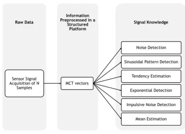
21 Figure 2.9. Above, structural representation of the classical approach of an algorithm
analysis and processing a signal from the raw data to obtain signal knowledge. Below,
representation of the proposed algorithm for the same purpose. 24
Figure 2.10. Representation of the segmentation process. 26
Figure 2.11. Representation of the S&L algorithm behaviour when applied to an aleatory
signal. 29
Figure 2.12. Flowchart of segmentation and labelling processes. 30
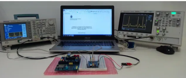
Figure 2.13. Representation of the assembly scheme. 31
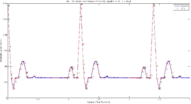
Figure 2.14. Graphical representation of the MATLAB simulation performance of the S&L
algorithm on an ECG Signal. 32
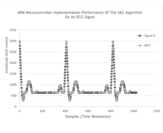
Figure 2.15. Graphical representation of the ARM microcontroller implementation
performance of the S&L algorithm on an ECG signal. 33
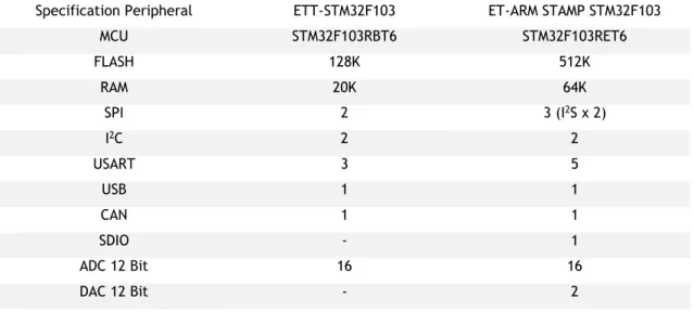
Figure 3.1. Module ETT-STM32F103 and RS-232 connection cable. 40
Figure 3.2. Module ET-ARM STAMP STM32. 41
Figure 4.1. Structural representation of the proposed algorithm for analysis and processing a
signal from the raw data to obtain signal knowledge. 46
Figure 4.3. Flowchart of Noise Detection function. 47 Figure 4.4. On the right, the generated noise signal; On the left, the generated DC signal. 48 Figure 4.5. Representative graph of the response from the Noise Detection Function when applied to a pure noisy signal with a sampling frequency equals to 100Hz and an
Interpolation error equals to 409 ADC levels. 50
Figure 4.6. Representative graph of the response from the Noise Detection Function when applied to a DC signal with a sampling frequency equals to 100kHz and an Interpolation error
equals to 10 ADC levels. 51
Figure 4.7. Flowchart of Sinusoidal Pattern Detection function. 52
Figure 4.8. Graphical representation of a 100 samples time window of the sinusoidal signal
test number 72. 56
Figure 4.9. Flowchart of Tendency Estimation function. 58
Figure 4.10. On the right, the scope image of a generated signal with a decaying tendency of 3.2Vpp of amplitude and 1.6V of offset; On the left, the scope image of a generated signal
with a rising tendency of 3.2Vpp of amplitude and 1.6V of offset. 60
Figure 4.11. Flowchart of Exponential Detection function. 61
Figure 4.12. On the right, the generated exponential stable signal-rising (class type “g”) in Burst Mode; On the left the generated exponential stable signal-decaying (class type “f”) in
Burst Mode. 63
Figure 4.13. Flowchart of Impulse Noise Detection function. 64
Figure 4.14. Cropping out the generation of the DC signal, with some random impulses
added, by ArbExpress software. 67
Figure 4.15. Cropping out the generation of the sinusoidal signal, with some impulses, by
ArbExpress software. 68
Figure 4.16. Flowchart of Mean Estimation function. 69
Figure A.1. Online developer platform. 83
Figure A.2. Available menus on the Mbed online compiler platform. 85
Figure A.3. Accessing the registered target board list. 85
Figure A.4. Selecting a platform. 85
Figure A.5. Selection of the destination Target. 86
Figure A.6.Creating a new project on Keil compiler. 87
Figure A.7. Exportation of a project from the Mbed platform to Keil. 88 Figure A.8. Opening on KEIL an exported project from the Mbed platform. 88
Figure C.1. Creating a new repository, in a directory, demonstration. 96
Figure C.2. Importation of files, from a project, demonstration 97
Figure C.3. Changing data log. 97
Figure C.4. Commit confirmation window. 98
Figure C.5. Verification of the revisions and changes list. 98
Figure C.6. One way to create a new user demonstration. 99
Figure C.7. Another way to create a new user demonstration. 99
Figure D.2. Signal creation on a Microsoft Office Excel file. 104
Figure D.3. Selecting a file format. 104
List of Tables
Table 1.1. Software development mechanisms requirements description. 7
Table 2.1. Standards advantages and disadvantages. 13
Table 2.2. Time to, computationally, calculate the orders of DFT vs. FFT. 15 Table 2.3. Graphic representation and brief description of the eight classes. 27 Table 2.4. Output return variables of the S&L algorithm application on an aleatory signal. 29
Table 2.5. Listing inputs and outputs of the MCT function. 30
Table 2.6. Input and Output of the MCT function. 33
Table 3.1. Comparison of the features specifications between two different STM modules. 41 Table 4.1. Listing inputs and outputs of the Noise Detection function. 47 Table 4.2. Results of the Noise Detection function applied to a pure noisy signal. 48 Table 4.3. Results of the Noise Detection function applied to a DC signal. 49 Table 4.4. Listing inputs and outputs of the Sinusoidal Pattern Detection function. 53 Table 4.5. Results of the Sinusoidal Pattern Detection function applied to a pure sine signal.
54 Table 4.6. Results of the Sinusoidal Pattern Detection function applied to a ramp signal. 55 Table 4.7. Listing inputs and outputs of the Tendency Estimation function. 58 Table 4.8. Results of the Tendency Estimation function applied to a signal presenting a rising
tendency. 59
Table 4.9. Results of the Tendency Estimation function applied to a signal with a presence of
a decaying tendency. 59
Table 4.10. Listing inputs and outputs of the Exponential Detection function. 61 Table 4.11. Results of the Exponential Detection function applied to a signal with a presence
of a rising exponential. 62
Table 4.12. Results of the Exponential Detection function applied to a signal with a presence
of a decaying exponential. 62
Table 4.13. Listing inputs and outputs of the Impulsive Noise Detection function. 65 Table 4.14. Results of the Impulse Noise Detection function applied to a DC signal with some
random impulses added. 66
Table 4.15. Results of the Impulse Noise Detection function applied to a sinusoidal signal
with some impulses. 66
Table 4.17. Results of the Mean Estimation function applied to a DC signal with some random
impulses added. 70
Table 4.18. Results of the Impulse Noise Detection function applied to a sinusoidal signal
List of nomenclatures
fs Sampling Frequency
µs Microseconds
A Amplitude of The Signal
B Frequency Band Limitation
c Propagation Velocity C Classes[ ] vector D Vertical Offset f Signal Frequency Hz Hertz k Wave Number kHz Kilohertz M Marks[ ] vector ms Milliseconds N Complex Multiples n Even Number N-1 Complex Adds ns Nanoseconds r Indices s Sparse representation s seconds T Times[ ] vector
Trend Relation between Maxima and Minima Tendency
Trendmax Tendency of Maxima
Trendmin Tendency of Minima
Wn Twiddle Factor
x Input Signal
x(k) Input Signal
X(k) Input Signal
x(t) Analog Input Signal
y Vector of Acquired Samples
λ Wave-Length
π Pi Value
Τ Signal Period
ψ Angular Frequency
Ω Highest Frequency
ω Phase Shift
List of Acronyms
ACoMS Autonomic Context Management
ADC Analog Digital Converter
API Application Programing Interface
ARM Acorn RISC Machine
ASCII American Standard Code For Information Interchange
CPU Central Processing Unit
CS Compressive Sensing
CSV Comma Separated Value
DC Digital Converter
DFT Discrete Fourier Transformation
ECG Electrocardiogram
FFT Fast Fourier Transform
IDE Integrated Development Environment
IEEE Institute of Electrical and Electronics Engineers
IoT Internet of Things
IS International System of Units
IT Information Technology
MCT Marks, Classes and Times vectors
NCAP Network Capable Application Processor
NIST National Institute of Standards and Technology
OS Operative System
POM Point of Measurement
PQ Power Quality
S&L Segmentation and Labelling
SI System of Information
SPIS Strategic Planning Information Systems
TEDS Transducer Electronic Data Sheet
TIM Transducer Interface Module
URL Uniform Resource Locator
Chapter
1
With the wider use of intelligent sensors, the need to apply them in network proved to be an asset, making them more efficient on data transfer by improving their methods of investigation. Considering the computational costs associated with data transmission, it will be quite useful to reduce the amount of data to send. So, the idea is to transmit less data and processing but acquire the same amount of information requiring fewer CPU resources. For this purpose, it is necessary to reduce the size of the sensor signal being processed and analyzed revealing how, in the world of sensors, intelligence is concentrated in measuring point within the transducer. In a final stage, it is also shown the organization of this document.
Chapter 1: Introduction
1. Introduction
The world, as it is known, is surrounded by new smart technologies that are rising every day, each one being related to a specific subject. All this electrical and electronic devices are used to solve different issues, ranging from the simplest one, such as domestic appliances, to the most complex that can be found in the industry. Sensors play an important role today. The way how they are adjusted depends from the context where they operate. In real-world applications, sensors are used for a wide range of purposes. One of those purposes is gathering data from the environment and, in this field, the communication among different types of devices becomes a necessity. To accomplish this task, embedded systems are being developed as Autonomic Context Management Systems (ACoMS) [1]. When in a context-aware application, a specific behaviour of an embedded system can be triggered if the system is described using a framework that models their sensing and data processing capabilities. Additionally, the appropriately setting of their dynamic composition enables, not only, their application in different context environments, but also, to perform the data transmission more effectively and efficiently. This translates the importance and necessity of communication between elements in both wired and wireless networks [2].
The application of sensors for complex signal processing, in the Point of Measurement (POM), requires improvements managing the information acquired by the sensors [1], [3]–[5]. A solution is to decrease the amount of data to process [1], [3]. This will aid, limited to the Central Processing Unit (CPU) characteristics, in monitoring the needed inputs whilst reducing waste, consumption, size, loss and costs. It will also allow us to know what to replaced or repair, and when, in the POM. In summary: to convert the information to a better format, with reduced size, in order to improve the performance of communication and storage mechanisms [1], [3]. However, the design of ACoMS poses several challenges [1]:
Integration: ability to fit in multiple computing environments enabling the sensor to respond to a wider range of applications;
Scalability: responsiveness of the data management collected, regardless of its size, amount or even its contextualization environment from which are acquired by the sensor;
Interoperability: configuration capability of the communication protocols in order to develop a more effective response, regardless of the context environment in which it is applied to a measuring for a posterior representation of the information;
Flexibility: data collection capacity with similar characteristics (such as type, data size, quantity, etc.) from different types of context sources in which the sensor is applied;
Chapter 1: Introduction
Reliability and Availability: attempting to implement the above capabilities may give rise to a number of potential losses of information or communication failures of the sensor.
Bearing in mind the objectives and operation policies, during the development of a system with an autonomic computing vision, the goal is to create a self-managing system that seamlessly supports both low-level sensing infrastructures and high-level adaptive applications. At the same time, the idea is to provide to the system, the development of an effective response for better performance. To provide that, it is necessary to optimize the operation of running in time domain and, to create the capacity of configuration and/or reconfiguration, of the application settings, on different levels of programming complexity [1], [3]. Parallel to the development of sensory instrumentation of measurement, the development of communication interactions contribute to the interoperability between devices of a common sensors network, whether wired or wireless, platforms and/or applications [6].
1.1. Work Background and Motivation
Several standards for sensor data processing already have been presented. The main goal was to extend the interoperability among sensors. Considering this, the National Institute of Standards and Technology (NIST) has proposed a family of standards as a universal solution [1], [3], [7]. This normalization effort establishes a standard of response to the challenge to preform connections and observed communication protocols among smart sensors, transducers and actuators, in different kinds of networks, wired or wireless, applied to different systems in numerous contexts. The IEEE 1451 family is a set of interfaces for smart transducers that define, not only a solution to the previously described challenges but also as a way to establish independent connections between those transducers, such as architecture description, message formats and software objects [1], [8], [9]. Given that, besides the instrumentation needed, it is also necessary to define the networks' control. An example of that is the signal analyses and processing field, where algorithms are required to process the acquired data in order to reduce its amount to subsequent transmission. As a complement to this, an electronic datasheet was defined to contribute for the sensor interoperability achieved with the plug-n-play architecture [6]. This datasheet intends to replace the paper version and includes, among many others, transducer identification, measurement units, data rage and scale, manufacturer-related information for the specific sensor, bandwidth and calibration details [3], [10]. When combined with the IEEE 1451 standards family, this electronic version of the datasheet is named Transducer Electronic Data Sheet (TEDS) and can present different levels of complexity [1], [9]. This combination allows not only the signal synthesis and analysis, but also the connection and communication among smart transducers
Chapter 1: Introduction
to validate the measurement procedure and exchange of information. Furthermore, it provides a platform that promotes the fusion of sensors knowledge. All the information acquired through data mining is by this way optimized and, as a consequence, so is the interaction between sensors and actuators with the real world [4], [11]. Embracing plug-n-play technology and its application to sensors, users can experience increased benefits, such as [6]:
More atomized and faster systems;
Faster and simpler system setup and configuration;
Improved efficiency and effectiveness of the measurements accuracy;
Increased diagnostics and troubleshooting;
Decreased time for repairing and/or replacing sensors;
Optimized sensor data management, bookkeeping and inventory management;
Automated use of calibration data for signals analysis and processing.
In this line of reasoning, the Internet of Things (IoT) is a new way to enable the exchange of signal information among sensors and transducers, from different manufacturers, in order to establish a dialogue among them. The information obtained from the sensors raw data and from the network states of the instrumentation helps to achieve higher reliability, since the key to achieve efficient and effective solutions for computer science problems is data representation [3], [4], [11]. As the main objective, the sensor needs to be smart enough to measure signal parameters. These led to the recognition of signal characteristics, allowing to study their general behaviour and to conclude about the type of the measured signal. Algorithms of signal analysis and processing can easily conceive this idea. For example, it is essential to know where signal segments are suitable for additional or time consuming processes like: high order statistics, wavelet, fuzzy logic, neural networks, spectrum analysis and any other signal processing technique. In other situations, such tasks are not adequate. For example, when the signal is constant [11]. Therefore, it is of great interest to know a few noteworthy information about the signal’s behaviour like: shape form; periodicity; amplitude; time constant; steady state value; tendency and future values; sampling frequency; mean and variance values; occurrence of impulsive noise and detection of patterns [3], [5], [11]. With all this, it is clear the importance that information has in our everyday lives. At the same time, the impact of Information Technology (IT) is a key element in achieving strategic and competitive advantages in the world of industry. Because of that, their respective implementation should be strategic and carefully planned and structured. Therefore, for us to take advantage of the potential of new technologies, it is necessary to make a large investment in software and hardware.
Chapter 1: Introduction
A System of Information (SI) is defined as an integrated set of resources (human and technological) whose objective is the proper satisfaction of all the information needs of software that wish, in short, process different inputs and produce various outputs in order to meet the objectives outlined. There is therefore a fundamental of the following characteristics:
Flexibility: ability to evolve face the prerequisites;
Reliability: reducing the occurrence of problems during operation; Organization: regards implementation needs;
Interaction: ease of use, allowing for a more friendly and intuitive interface.
The proper functioning of the systems is crucial and because of that, before starting any process of development of information systems architecture components, it is crucial that it can be conceived from a global point of view. Thus, it is possible to ensure complete integration between the components and the prioritization of their implementation, which is the working part of a Strategic Planning Information Systems (SPIS). The SPIS defines the components of a SI, working as a guide for all future interventions. As a process, after the definition of the global strategy and the identification of components needed to develop their achievement goes to the field of software engineering. This area receives information support from the following areas: systems analysis, project management, scheduling and quality control. Thus, the activities associated with software engineering can be grouped into three broad phases, according to its goal of development and operation: design planning, implementation and maintenance.
Developing a software is a very complex process. For this reason, it is divided into a set of activities less complex. Its uniform execution, partially ordered, leads to the production of software. As for the study of its features, this is ensured by software engineering studies. Therefore, to obtain a quality software, it is necessary to respond and accomplish the technical requirements and the following mechanisms from Figure 1.1:
Chapter 1: Introduction
Figure 1.1. Stages of software development mechanism.
The requirements of each software development mechanism are described in Table 1.1:
Table 1.1. Software development mechanisms requirements description.
Mechanisms of Software Development Description
Requirements Specification
Describes the software that will be written accurately, preferably in a mathematically rigours way. Therefore, the activities involved include identifying:
The general purpose of the system; The project objectives;
The technical restrictions;
The problems and associated risks;
The definition of the project control process; The most relevant functions and implementation
of alternatives, carrying out their assessment and selection;
The presentation of findings and
recommendations with technical justification, functional and financial;
Preparing and obtaining the approval of the project plan (identification of tasks, making diagrams, etc.). Software Development Mechanism Requirements Specification Software Architecture Design Implementation Test Documentation Technical Support Maintenance
Chapter 1: Introduction
Software Architecture Design
Abstract representation of the system meets the product requirements, but also ensures that future requirements can be satisfied. Directs the interfaces between software systems and other software products, as well as with the basic hardware or operating system.
Implementation
Transformation of the project in source code. Although, it is the most obvious part of the software engineering work, but does not mean necessarily that is the major portion of it.
Test
Test, step by step, each part of the system. Several activities ate performed in order to validate the software product in different situations, testing each feature of each module, taking into account the specification made in the design phase. As result, the test report contains all relevant information about the founded errors in the system, and their behaviour in various aspects.
Documentation
Serves as technical support to internal software project for future purposes, such as maintenance and enhancements.
Technical Support
Development of technical material to support the implementation of the software by users. The datasheets and user guides are great examples of this material. The great advantage of this phase is making of the users to submit questions and identify problems in the software performance, which leads to the next stage.
Maintenance
Reviewing and improving the software, dealing with the problems and requirements of the previous stage. It may take more time that the one spent on the initial development phase. Apart from the possibility of being required to add code to match the original design, it may also be necessary to determine how the software will work after maintenance.
Chapter 1: Introduction
That said, it can be concluded that these are necessary to support certain types of technical development, such as:
Model before performing;
Estimate several factors before proceeding;
Test and measurement before, during and after production;
Carry out the study and analysis of risk factors.
The applications of these techniques must be rigorous, systematic, efficient and controllable. Naturally, the effectiveness of this process also instils the use of tools to support the process. Thus, the benefits associated with innovative functional use are:
Reduction of operating costs by automating and reformulation processes;
Satisfaction of information requirements of users;
Contribution to the creation of new products and services;
Improving the effectiveness of decision support methods;
Improve and increase the level of service provided to customers;
Improve and automate the performance of electronic devices.
This document is structurally divided into five chapters. The first chapter conducted a background study and work motivation to the present project proposal. The second chapter will be made respective theoretical considerations in the area of acquisition, analysis and signal processing. There will also be presented some examples of techniques and theorems applied to the study area. In a final stage, will be also described a proposal of new algorithm for the same purpose. In the third chapter, it will be briefly exposed both hardware and software tools applied to support the development and production of the project, flaunting their environments and interfaces, as well as its features and specifications. In the fourth chapter, it will be performed a depth study of the algorithm performance and of the integral parts of the project, that is, not only will be described the specifications of each Application Programming Interface (API) function, but also an experimental setups and their respective analysis. In the fifth and final chapter, the final remarks will be made, as well as the general conclusions of the project and suggestion of some future prospects.
Chapter
2
Parallel with the implementation of various patterns, these are also being developed to extend a greater interoperability between sensor systems. Here, will be explored a subset of multiple sensors standards. The IEEE 1451 is a set of standards developed to unify the various standards and protocols, providing a basic protocol. It will be studied the characteristics of the IEEE 1451.0 standard, where the communication of all networked transducers is ensured by TEDS, with the same format for all sensors and actuators for both networks, wired or wireless. They will also be discussed some of the more popular methods of acquiring and presented a more effective proposal to effect answering the need to reduce computational cost while maintaining the same amount of processed information.
Chapter 2: Hardware and Software Development Tools
2. Theoretical Considerations on Sampling and
Measurement
Traditionally, the sampling technics follow the Nyquist-Shannon theorem. This allows a reliable reconstruction and/or reproduction of the signal, image or video. If a signal is to be reconstructed from acquired samples, the signal should have a finite bandwidth and must be sampled with a sampling frequency (fs) at is least equal to twice highest frequency (Ω) presented in the signal. It is possible to express this requirement using equation (2.1) [12]:
𝒇𝒔 = 𝟐 × 𝜴
(2.1)
In most cases, the signals doesn’t owns the requisite aforementioned, but nonetheless, despite the absence of information affecting the tail side of the spectrum, generally, the error resulting in the reconstruction of the signal is acceptable. To solve this problem a filter is used, before the digital to analogue converter, with an acceptable fs as mentioned above [12]. The notion of taking less data but acquiring the same information does not apply to the acquisition of the whole waveform, instead of that, the algorithm only keeps some of the samples. Each sample carries a part of the whole information. This notion proves to be enough for the execution of the proposed algorithms for analysis and signal processing for sensors developed for both wired or wireless networks, with intelligence distribution of intelligence and computational capabilities [3]. Standards based approaches offer, despite some disadvantages, advantages over proprietary solutions as presented on Table 2.1 [8]:
Table 2.1. Standards advantages and disadvantages.
Advantages Disadvantages
Sensor architecture defined; Software flexibility; Firmware functions; Universal applications.
Firmware programming in object-oriented language style;
Increase of the algorithm complexity in case of the embedded controller doesn’t support
this type of language;
Become burdened by the amount of memory required to instantiate objects in the
Chapter 2: Hardware and Software Development Tools
The literature presents several algorithms to overcome the bridging gaps created by the disadvantages presented. Among them, as was previously mentioned, there are different levels of complexity that characterize the algorithms. Within the most complex, as the best known it stands out the Fast Fourier Transform (FFT) algorithm, but there are many others, like for example the Compressive and Sensing (CS) algorithm. Observing low computational algorithms requirement, there is an algorithm that by Segmentation and Labelling (S&L) of acquired samples, during the sampling process, facilitates the raw data mining process by having the same signal information distributed by fewer samples (the most significant). Additionally, based on the sensor information, allows the adaptation of algorithm to the application context in which it is inserted [3], [10].
The next three subsections will present a description of how these algorithms work using a smart sampling process. The first one, is a well-known measurement procedure [2]. The second one, is a technique that takes, randomly, a fixed number of samples from a signal [3]. The third one, a new algorithm is proposed for information extraction from samples of a signal. Suited for data mining process and adapted to sensor signals where a control algorithm is applied based on a technique that process acquired signal samples in order to generate a set of three vectors, constituted by raw information [3], [10]. Divided into two different stages, segmentation and labelling, it will be possible to understand how it is possible to extract parameters from an oversampled signal, allowing the induction of its global behaviour by applying six distinct functions presented in the fourth chapter of this document [4], [11].
2.1. Fast Fourier Transform
The present algorithm, one of the most important amid the best known, presents as the main goal to calculate efficiently the frequency contents of signals. Being this an algorithm developed for analysis and processing signals through microcontrollers and microprocessors, is a fast computational algorithm to perform numerically and an efficient way for the calculation of the Discrete Fourier Transform (DFT), where its big difference is the time complexity. The basic concept is taking an array in time domain, Td seconds, of samples and
processes it using the Fast Fourier Transform (FFT) algorithm, in order to produce a new array in frequency domain, Bb Hz (bidirectional bandwidth). This last one is a spectrum of samples.
Both arrays present exactly the same number of samples. Real value samples are received by the input of the algorithm that return in the output side complex value samples [13]–[15]. Actually, there are several ways to implement the FFT algorithm, although some require many resources, other are more simply and not optimized. Thus, through the literature, the idea is to describe, briefly, how to perform an analysis and processing of a signal using an implicit Fourier analysis on mathematical methods. Therefore, the chosen technique, presented by Cooley and Tukey in 1965, the DFT can be determined using equation (2.2) [14]:
Chapter 2: Hardware and Software Development Tools
𝑿(𝒌) = ∑ 𝒙(𝒏) × 𝒆−𝒊𝟐𝝅𝑵 𝒌𝒏 𝑵−𝟏
𝒏=𝟎
(2.2)
Assuming that x(n) and X(k) are periodic input signal, and exploring the symmetries of the complex e−i2πNkn, conventionally defined as a twiddle factor WN= e−i
2π
N and this is like saying that in an a unit circle from Figure 2.1 one has that [14]:
Figure 2.1. WN representation on a unit circle.
Then, in equation (2.2), the twiddle factor can be conjugated to get equation (2.3) [14]:
𝑿(𝒌) = ∑ 𝒙(𝒏) × 𝑾𝑵𝒌𝒏
𝑵−𝟏
𝒏=𝟎
(2.3)
Where k ∈ ℝn can assume values on the interval 0 up to N − 1 considering how much
computational is involved, it takes N2 complex multiplies and N(N − 1) complex additions, to
get each X(k) value. In this way, considering O(N2) order of computations for direct DFT and O(Nlog2N) order for FFT, it can be seen on Table 2.2, the FFT will be reduce considerably
[13], [14]:
Table 2.2. Time to, computationally, calculate the orders of DFT vs. FFT.
Order of Computations Necessary Number of Operations to Compute FFT
N 103 106 109
N2 106 1012 1018
N log2 N 104 20*106 30*109
Seeing each operation in nanoseconds (ns) that is, each operation took a nanosecond, 1018ns
Chapter 2: Hardware and Software Development Tools
how much greater is wNkn, bigger is the difference between both orders. Consequently, in
order to reduce the number of operations to the order O(Nlog2N) the FFT algorithm is
applied. To make it possible, the idea is to do decompositions into smaller DFTs; execute the simplifications like wNkn which is equals to 1 and wN
N
2(k) which is equals to −1. This will reduce computation complexity; reminding the periodicity on the input, assimilate that wN
n(k+N)
= wNk(n+N)= wNkn and wN
k(N−n)
= wN−kn=
(
wNkn)
∗. After these steps, the first phase can be called asdecimation in time, where n is an even number. In this way, considering equation (2.3), lets
split the sum into the even entries of x, to get equation (2.4) [14]:
𝑿(𝒌) = ∑ 𝒙(𝒏) × 𝑾𝑵𝒌𝒏
𝒏 𝒆𝒗𝒆𝒏
+ ∑ 𝒙(𝒏) × 𝑾𝑵𝒌𝒏
𝒏 𝒂𝒅𝒅𝒊𝒕𝒊𝒐𝒏𝒂𝒍
(2.4) If n is an even number, it can be consider as 2r, resulting in equation (2.5) [14]:
𝑿(𝒌) = ∑ 𝒙(𝟐𝒓) × 𝑾𝑵𝟐𝒓𝒌 𝑵 𝟐−𝟏 𝒓=𝟎 + ∑ 𝒙(𝟐𝒓 + 𝟏) × 𝑾𝑵(𝟐𝒓+𝟏)𝒌 𝑵 𝟐−𝟏 𝒓=𝟎 (2.5)
At this point, what was done is rename the index calling it Radix-2. Mathematically simplifying equation (2.5) it is obtained equation (2.6) [14]:
𝑿(𝒌) = ∑ 𝒙(𝟐𝒓) × (𝑾𝑵𝟐)𝒓𝒌 𝑵 𝟐−𝟏 𝒓=𝟎 + 𝒘𝑵𝒌 ∑ 𝒙(𝟐𝒓 + 𝟏) × (𝑾𝑵𝟐)𝒓𝒌 𝑵 𝟐−𝟏 𝒓=𝟎 (2.6)
Looking again to the unit circle, from Figure 2.1, but this time replacing the value N by 8, results in Figure 2.2 [14]:
Chapter 2: Hardware and Software Development Tools
Observing Figure 2.2 it can be modified equation (2.6) so they look like two shorter DFTs represented by equation (2.7) [14]: 𝑿(𝒌) = ∑ 𝒙(𝟐𝒓) × (𝑾𝑵 𝟐) 𝒓𝒌 𝑵 𝟐−𝟏 𝒓=𝟎 + 𝒘𝑵𝒌 ∑ 𝒙(𝟐𝒓 + 𝟏) × (𝑾𝑵 𝟐) 𝒓𝒌 𝑵 𝟐−𝟏 𝒓=𝟎 (2.7) Where ∑ x(2r) × (wN 2) rk N 2−1 r=0 is the length N
2 DFT of even entries and ∑ x(2r + 1) × (WN2) rk
N 2−1
r=0 is
the length N
2 DFT of additional entries. Each one can be written on a compact way G(k) and
H(k), respectively, getting equation (2.8) [14]:
𝑿(𝒌) = 𝑮(𝒌) + 𝒘𝑵𝒌 𝑯(𝒌) (2.8)
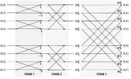
At this point, considering that one wants to compute N equals to 6, k = [0, 2, 4, 6] are the even entries and k = [1, 3, 5, 7] are the additional entries, to get the final X(k) where k = [0, 1, 2, 3, 4, 5, 6, 7]. With this, the DFT value calculation is shown on Figure 2.3 [13], [14]:
Figure 2.3. Radix-2 Fast Fourier Transforms, Butterfly algorithm.
There are no need to stop here. Keeping the same even and additional entries, it is still possible to simplify Figure 2.3 as shown on Figure 2.4 [13]–[15]:
Chapter 2: Hardware and Software Development Tools
Figure 2.4. Radix-4 Fast Fourier Transforms, Butterfly algorithm.
Now, confronting Figure 2.4 with Figure 2.2 and replacing the required values, it is obtained Figure 2.5 [13], [14]:
Figure 2.5. Substitution by the unit circle value and divide in three stages of decomposition.
With this, it is possible to conclude how much decomposition it is possible to do. If N is a power of 2, it is decomposed the DFT into log2N stages. Which means that is achieved Nlog2N computational multiplies. This explains the previously mentioned speeds difference between the DFT and the FFT, making the FFT algorithm the fastest in a computational way. Bearing in mind the computational storage, to compute the length of DFT, pth and qth values in the
(m − 1)st (first) stage are used to get pth and qth values in the mth stage. In this way, it can be
done by what is called “in place” which means no extra storage. Then, to arrange the input value may be placed in an algebraic perspective, getting the Figure 2.6 [13], [14]:
Chapter 2: Hardware and Software Development Tools
Figure 2.6. Algebraic representation of the computational storage.
Appreciating the grey background, both are equal but negative to each other, except for the first column only. It is possible to rewrite it in a simple way as given on Figure 2.7 [12]:
Figure 2.7. Calculating the Fourier matrix.
Now, taking a time domain signal, it can be separated it in smaller and smaller pieces by applying a strategy called Decimation in Frequency FFT. Considering again equation (2.1), the even samples of X(k) are given by equation (2.9) [13]:
𝑿(𝟐𝒓) = ∑ 𝒙(𝒏) × 𝑾𝑵𝟐𝒏𝒓
𝑵−𝟏
𝒏=𝟎
(2.9)
Where r ∈ ℝn can assume values in the interval from 0 up to N−1
2 . Splitting equation (2.8)
into two half parts of elements, getting equation (2.10) [13]:
𝑿(𝟐𝒓) = ∑ 𝒙(𝒏) × 𝑾𝑵𝟐𝒏𝒓 𝑵 𝟐 ⁄ −𝟏 𝒏=𝟎 + ∑ 𝒙(𝒏) × 𝑾𝑵𝟐𝒏𝒓 𝑵−𝟏 𝒏=𝑵 𝟐⁄ (2.10)
Chapter 2: Hardware and Software Development Tools 𝑿(𝟐𝒓) = ∑ 𝒙(𝒏) × 𝑾𝑵 𝟐 𝒏𝒓 𝑵 𝟐 ⁄ −𝟏 𝒏=𝟎 + ∑ 𝒙(𝒏 +𝑵 𝟐) × 𝑾𝑵 𝟐(𝒏+𝑵𝟐)𝒓 𝑵 𝟐 ⁄ −𝟏 𝒏=𝑵 𝟐⁄ (2.11)
Again, can be made a few simplification to get equation (2.12) [13]:
𝑿(𝟐𝒓) = ∑ 𝒙(𝒏) × 𝑾𝑵 𝟐 𝒏𝒓 𝑵 𝟐 ⁄ −𝟏 𝒏=𝟎 + ∑ 𝒙(𝒏 +𝑵 𝟐) × 𝑾𝑵𝟐 𝒏𝒓 𝑵 𝟐 ⁄ −𝟏 𝒏=𝑵 𝟐⁄ (2.12)
That can be simplified as expressed by equation (2.13) [13]:
𝑿(𝟐𝒓) = ∑ [𝒙(𝒏) + 𝒙 (𝒏 +𝑵 𝟐)] × 𝑾𝑵𝟐 𝒏𝒓 𝑵 𝟐 ⁄ −𝟏 𝒏=𝟎 (2.13) This is like a N
2 DFT of summed input. The additional samples of X(k) can be showed by
equation (2.14) [13]: 𝑿(𝟐𝒓 + 𝟏) = ∑ [𝒙(𝒏) + 𝒙 (𝒏 +𝑵 𝟐)] × 𝑾𝑵𝒏× 𝑾𝑵 𝟐 𝒏𝒓 𝑵 𝟐 ⁄ −𝟏 𝒏=𝟎 (2.14)
Finally, it is obtained the decimation in time that both of them are most likely equivalent. As a conclusion, it can be done a series of DFT just by performing some stages and for each stage it can be made as showed on Figure 2.5. The number of necessary stages is directly dependent of the DFT length [13], [14].
2.2. Compressive Sensing Technique
The mains goals of the present algorithm aims to investigate the applicability of the CS technique in Power Quality (PQ) measurement. In particular, it will be study the ability of the given measurement accuracies comparable with standard requirements and typical PQ measurement methods; the capacity to reduce the required memory with respect to traditional measurement methods; and the transformation of raw data information in other domains
[3], [12]
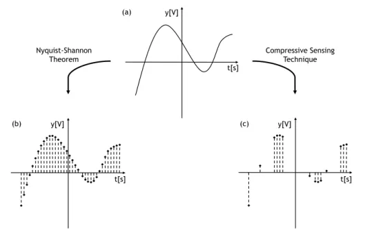
. In this way, it is possible to represent the signal using a small number of samples that are acquired with a step of aleatory sampling. In order to apply this technique, to enable their representation on is destiny domain, it is necessary to choose the right expansion basis for 𝑚 samples acquired. These 𝑚 samples are just a few samples, and from them, only a few are meaningful. The Figure 2.8 represents the acquisition of the same signal (a) using two different techniques: (b) acquisition of 𝑛 samples equally spaced and observing the Nyquist-Shannon theorem and (c) acquisition of 𝑚 random samples using the CS technique [3].Chapter 2: Hardware and Software Development Tools Nyquist-Shannon Theorem Compressive Sensing Technique (a) (b) (c) y[V] y[V] y[V] t[s] t[s] t[s]
Figure 2.8. Representation, in time domain, the acquisition of samples from the signal (a), observing the Nyquist-Shannon theorem (b) and using the Compressive Sensing technique (c).
Considering the time domain, it is possible to express the mechanism of sampling using equation (2.15) [3], [12]:
𝒚 = 𝝓 × 𝒙 (2.15)
Where y ∈ ℝm represents the vector for measures, x ∈ ℝn correspond to the input signal and
ϕ is a sampling [n × n] matrix [11]. Comparing the number n and m of samples acquired, m is much smaller than n (m ≪ n) but samples are enough to reconstruct the signal, as explained before. Given by this, the CS algorithm can reduce the amount of data being transmitted but, simultaneously, having exactly the same information as it was previously mentioned above as being an ideal idea. The compression of data is available due to the fact of having a wide set of signals that have a sparse representation. With this in mind, it is possible to express x ∈ ℝn
using equation (2.16) [3], [12]:
𝒙 = 𝝋 × 𝒔 (2.16)
Where s ∈ ℝn correspond to a sparse representation of the signal x on the orthonormal basis
φ [n × n]. Comparing the CS algorithm with the traditional techniques for data compression, Nyquist-Shannon sampling theorem, it is noted that the transformed signal s is then computed
from x, which means a proper orthonormal bases, and the sparse significant coefficients are
adaptively singled and retained [12]. With this, on the signal reconstruction stage, the original signal is obtained by inverse transformation of those coefficients [11]. Combining the two previous equations (2.15) and (2.16), it is now possible to express the vector of the
Chapter 2: Hardware and Software Development Tools
acquired samples y ∈ ℝm according to the representation of the sparse representation of the
signal x, using equation (2.17) [2]:
𝒚 = 𝝓 × 𝝋 × 𝒔 = 𝒁 × 𝒔 (2.17)
The system of equations presented above has an infinity number of solutions. To perform a
CS with efficient success, the matrices ϕ and the orthonormal basis matrix φ need to be incoherent. Eventually, if the s is sufficiently sparse and the system of equations can be solved, providing a single solution [2]. By this is possible to affirm that the CS algorithm allows both acquisition and compression operations on a unique step and, accurately reconstruct a signal from a few samples [11].
2.3. Segmentation and Labelling Method
The increased demand for intelligent systems is able to provide more and better capabilities and features encouraged by the development of smart sensors and embedded devices that are capable of communicating directly with each other’s. Thus, the exchange of data measured by the system itself, introduced more flexibility to the intelligent transducer, thereby improving overall system performance [9]. Intelligent devices such as sensors and actuators with digital outputs have been improved, not only in terms of performance but also in terms of reducing computational cost. By this way, the smart sensors components, including signal conditioners, communication microcontrollers and electronics have also been improved [7]. As grounded already, in Chapter 1 of this dissertation, the family of IEEE 1451 standard defines a set of communication interfaces to interconnect electronic devices such as sensors, actuators and transducers with systems with embedded microprocessors. In addition, they also provide protocols used by applications in both networks, wired or wireless [16]. The IEEE 1451.0 standard provides a set of common features, simplifying the creation of standards for different interfaces. At the same time the interoperability among members of this family is maintained [9], [16]. This interoperability is ensured by the TEDS, because it contains the necessary calibration data and operating methods to create a calibrated results observing the standard International System (IS) of units [7]. The main objective of this set of standards is to structure the interoperability of elements that integrate a system allowing the existence of transducers with plug-and-play features. With this, it is possible to reduce or even eliminate errors of Human origin, which sometimes occur. The IEEE 1451.0 defines the actions that must be performed by a Transducer Interface Module (TIM) and the common features to all devices implementing it [17]. Furthermore, this family of standards also specify formats for the TEDS and defines a set of commands to facilitate control of the TIM, as well as, also provide supplementary information to the application every time the systems needs to read or write data. The information is passed between the Network Capable Application Processor (NCAP) and the TIM through the software interface on a common hardware. The software
Chapter 2: Hardware and Software Development Tools
interface is defined by the IEEE 1451 standard. The task of adding new transport interfaces is simplified. In order to enable communications, it was created the API [7], [9]. In this section, a new method for analysis and signal processing will be presented, as well as, the evaluation of its performance. The S&L algorithm names the method and formulates a proposal for a new version of the IEEE 1451 standard [2].
The idea of performing analysis and processing a digital signal involves the extraction of knowledge from raw data. To produce this effect, as have been described in the previous sections, there are several methods. Some of them are more efficient than others. Despite its advantages and disadvantages, generally, they are all very sensitive to the presence of noise and other artefacts in the signal. The majority of signal analysis algorithms focuses on acquiring data and apply directly processing methods, in order to extract the data information. The method presented here attempts to go beyond, proposing an algorithm applicable to smart sensor, whose performance must be the image and likeness of a human being. In other words, the main objective is that the algorithm recognizes a signal and gets the same conclusions estimated by the Human observer [4], [11]. To achieve this task, the algorithm focuses on getting an intermediate stage after signal acquisition. This consists of introducing a processed data structure to subsequently allow for their examination [17]. Generally, the conversion of data domain acquired for obtaining information from the data by detecting specific patterns involve a high computational cost. Thus, the importance of a standardized structure proves to be an asset when, at the outset, it presented several goals. With this, we abdicate the necessity of return to the original acquired samples, and go through the processing stage, each time we intend to apply a function of the algorithm. In Figure 2.9 is represented the distinction between the most conventional methods and the technique proposed here enhancing, notably, a considerable reduction in the computational cost [17].
Chapter 2: Hardware and Software Development Tools
Signal Knowledge Information Non Processed
Raw Data Sensor Signal Acquisition of N Samples Processing Procedure
Function A Function B Function C … Function N
Most Common Algorithms Signal Knowledge Information Preprocessed Raw Data Sensor Signal Acquisition of N Samples Structured Platform
Function A Function B Function C … Function N
Segmentation and Labeling Algorithm
Figure 2.9. Above, structural representation of the classical approach of an algorithm analysis and processing a signal from the raw data to obtain signal knowledge. Below, representation of the
proposed algorithm for the same purpose.
As can be observed in Figure 2.9, the algorithm here proposed has a layered structure where the output of one stage is the respective input of the next [11]. Due to the variety of functions provided by the signal processing technique presented here, it can be applied to any type of signal.
The method begins by performing a signal sample acquiring a defined set samples, according to the aforementioned sampling theorem of Nyquist-Shannon [3], [17]. Then it performs a pre-processing of the signal, in the time domain, obtaining a uniform platform with embedded information, from which a homogeneous analysis according to the intention of the same application is possible [17]. The platform will also allow the detection of waveforms from small isolated features that lead to signal characteristics extraction and, consequently, signal recognition.
Now, the interaction of the segmentation process, followed by the raw information labelling process, are involved in getting this intermediate stage and how this sampling proposed technique focuses up to emulate an human observer, to infer the overall performance of the sampled signal [4], [17].