TECHNICAL UNIVERSITY OF LISBON
SCHOOL OF ECONOMICS AND MANAGEMENT
MASTER OF SCIENCE IN FINANCE
PROJECT
PORTFOLIO INSURANCE: A COMPARISON
OF ALTERNATIVES STRATEGIES
JORGE FILIPE BAPTISTA DA COSTA
Supervision: Professora Doutora Raquel M. Gaspar
Jury:
President: Professor Doutor João Duque
Members: Professora Doutora Raquel M. Gaspar
Mestre Pedro Rino Vieira
ii PORTFOLIO INSURANCE: A COMPARISON OF ALTERNATIVE STRATEGIES
Jorge Filipe Baptista da Costa
M.Sc: Finance
Supervision by Raquel M. Gaspar
Abstract
This study makes a comparison between the most popular strategies of Portfolio Insurance based on Monte Carlo simulation. This work aims to define the best strategy at comparing different strategies and provide a contribution to solving some divergences in literature. Most of the previous comparisons do not take into consideration all the strategies discussed in this study and this analysis intends to add some relevant findings. The OBPI, CPPI and SLPI strategies are evaluated in terms of moments of the distribution, performance ratios (Sharpe ratio, Sortino ratio, Omega ratio and Upside Potential ratio) and stochastic dominance in different market conditions represented by an underlying asset that follows a geometric Brownian motion. In order to have a perception of a real situation in financial markets, the strategies are later also applied to three major stock indices.
We find that CPPI 1 and SLPI strategies should be preferred in all scenarios according to the higher performance ratios, the higher expected returns and other measures. The choice between them is based on the preferences of the investor or manager, but we also find that the CPPI 1 strategy stochastically dominates, on second and third order, the others strategies in bear market scenarios. From our results we can state that a value of 100% for the floor should be preferred in terms of performance ratios, expected returns and other measures. This comparison allows improving the efficiency of decision making of an investor or manager in a Portfolio Insurance investment.
iii PORTFOLIO INSURANCE: A COMPARISON OF ALTERNATIVE STRATEGIES
Jorge Filipe Baptista da Costa
Mestrado em Finanças
Orientação de Raquel M. Gaspar
Resumo
Este estudo realiza uma comparação entre as estratégias mais populares de
Portfolio Insurance, através da Simulação de Monte Carlo. Este trabalho tem como objectivo definir a melhor estratégia através de diversas comparações e dar um contributo para resolver algumas divergências na literatura. A maioria das comparações realizadas anteriormente não têm em consideração todas as estratégias presentes neste estudo e esta análise pretende acrescentar algumas conclusões relevantes.
As estratégias OBPI, CPPI e SLPI são avaliadas através dos momentos da distribuição, rácios de desempenho (Sharpe ratio, Sortino ratio, Omega ratio e Upside Potential ratio) e dominâncias estocásticas nas diversas condições de mercado representadas pelo activo subjacente que segue um movimento Browniano geométrico. De forma a ter uma compreensão da realidade dos mercados financeiros, as estratégias também são aplicadas a três dos maiores índices de acções.
Concluímos que as estratégias CPPI 1 e SLPI devem ser preferidas em todos os cenários devido aos elevados rácios de desempenho, elevadas rendibilidades esperadas e a outras medidas. A escolha entre as duas estratégias é feita com base nas preferências do investidor ou gestor, mas também concluímos que a estratégia CPPI 1 domina estocásticamente, a segunda e terceira ordem, todas as restantes estratégias em cenários de mercado bear. De acordo com os resultados obtidos podemos afirmar que um floor
de 100% deve ser escolhido devido aos resultados dos rácios de desempenho, rendibilidades esperadas e outras medidas. Esta comparação permite melhorar a eficiência da tomada de decisão de um investidor ou gestor num investimento de
Portfolio Insurance.
iv
Acknowledgments
First, I would like to thank my supervisor, Professor Raquel M. Gaspar, for all the support from the beginning with, comments, suggestions and for the research idea underlying this project. All of this support contributed to make this study more interesting.
I would to thank to all friends and colleagues that I shared this step by the incentives and support that they gave me to face all the concerns and difficulties over time.
I would like also to thank to Carolina, for all unconditional support across the entire process, and especially in most difficult times.
At last, I would like to thank all my family and especially to my parents, who have made this Master a reality.
v
Table of Contents
Abstract ... ii
Resumo ... iii
Acknowledgments ... iv
Table of Contents ... v
List of Tables ... vi
List of Figures ... vii
1 Introduction ... 1
2 Review of Literature ... 3
2.1 Portfolio Insurance ... 3
2.2 Option Based Portfolio Insurance - OBPI ... 4
2.3 Constant Proportion Portfolio Insurance - CPPI ... 4
2.4 Stop-Loss Portfolio Insurance - SLPI ... 5
3 Methodology ... 6
3.1 Monte Carlo Simulation ... 6
3.2 The Procedure and Parameters ... 7
4 Results ... 10
4.1 The First Four Moments ... 10
4.2 Ratio Analysis ... 13
4.3 Other Measures ... 17
4.4 Stochastic Dominance ... 20
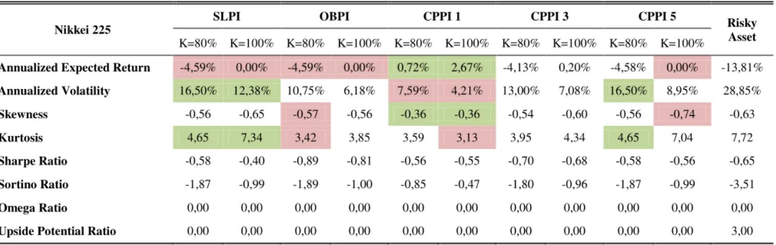
4.5 Applying Strategies to World Stock Indices ... 25
5 Discussion ... 29
5.1 Normal and Bull Market Scenarios ... 29
5.2 Bear Market Scenarios ... 30
5.3 Other Main Findings ... 31
6 Conclusions and Further Research ... 32
References ... 34
Appendix A ... 37
vi
List of Tables
1 Market Scenarios ... 8
2 Annualized Expected Returns ... 11
3 Annualized Volatilities (Standard Deviations) ... 12
4 Relative Skewness ... 12
5 Relative Kurtosis ... 13
6 Sharpe Ratios ... 15
7 Sortino Ratios ... 15
8 Omega Ratios ... 16
9 Upside Potential Ratios ... 16
10 Probability to have the portfolio value ≤ K + 5% during the investment period ... 18
11 Probability to have a the portfolio value > 5% risk-free investment ... 19
12 Stochastic Dominance – First Order ... 22
13 Stochastic Dominance – Second Order ... 23
14 Stochastic Dominance – Third Order ... 24
15 Performance Results – S&P 500 ... 26
16 Performance Results – DJ EuroStoxx 50 ... 26
17 Performance Results – Nikkei 225 ... 26
vii
List of Figures
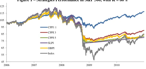
1 Strategies Performance in S&P 500, with K = 80% ... 27
2 Strategies Performance in S&P 500, with K = 100% ... 27
3 Strategies Performance in DJEuroStoxx 50, with K = 80% ... 27
4 Strategies Performance in DJEuroStoxx 50, with K = 100% ... 28
5 Strategies Performance in Nikkei 225, with K = 80% ... 28
6 Strategies Performance in Nikkei 225, with K = 100% ... 28
A.1 Return Distributions with scenario: μ = -15% and σ = 15% ... 37
A.2 Return Distributions with scenario: μ = -15% and σ = 40% ... 38
A.3 Return Distributions with scenario: μ = -5% and σ = 15% ... 39
A.4 Return Distributions with scenario: μ = -5% and σ = 40% ... 40
A.5 Return Distributions with scenario: μ = 5% and σ = 15% ... 41
A.6 Return Distributions with scenario: μ = 5% and σ = 40% ... 42
A.7 Return Distributions with scenario: μ = 15% and σ = 15% ... 43
A.8 Return Distributions with scenario: μ = 15% and σ = 40% ... 44
B.1 Stochastic Dominance – First Order, with K = 80% ... 45
B.2 Stochastic Dominance – Second Order, with K = 80%... 46
B.3 Stochastic Dominance – Third Order, with K = 80% ... 47
B.4 Stochastic Dominance – First Order, with K = 100% ... 48
B.5 Stochastic Dominance – Second Order, with K = 100%... 49
1
Chapter 1
Introduction
The first Portfolio Insurance strategies appeared at the end of the 70‟s in the
financial industry. Leland and Rubinstein (1976) implemented the first Portfolio Insurance strategy called Option Based Portfolio Insurance (OBPI) which combined a listed put and an investment in the underlying asset. Later, Perold (1986) introduces the Constant Proportion Portfolio Insurance (CPPI) and after that many authors contribute to the development of these strategies. The Stop-Loss Portfolio Insurance (SLPI) was used by Rubinstein (1985) in a Portfolio Insurance context. The Portfolio Insurance had a high development in recent decades but always with the aim of creating new solutions to allow the investors limit the downside risk of the portfolio while preserving the upward potential. This study is based on a comparison between the Portfolio Insurance strategies more relevant in literature (CPPI, OBPI and SLPI) in order to identify the best strategy under different market situations.
Therefore, many authors have been dedicated to study new adaptations of the strategies (see for example Cont and Tankov (2007)) or to make comparisons based on theoretical assumptions (see for example Bertrand and Prigent (2005)). However, there are also some authors who have been doing empirical analysis on these strategies but were yet to be studied different combinations of parameters of the strategies and underlying assets. (see for example Annaert et al. (2009)).
Among the studies that compare Portfolio Insurance strategies, the most well known are the following. Black and Rouhani (1989) compare CPPI and OBPI and find that OBPI has better performance than CPPI under a moderate market increase, but under small or large increases and market declines, the CPPI is better than OBPI. Cesari and Cremonini (2003) compare nine different strategies and conclude that CPPI has better performance in bear and no-trend markets. Bertrand and Prigent (2005) compare OBPI to CPPI assuming that the risky asset follows a geometric Brownian motion and find that OBPI dominates CPPI in terms of mean-variance, but CPPI has less downside risk and is high positively skewed. Khuman et al. (2008) show that the CPPI 3 and 5 have poorly performances compared with CPPI 1 for volatilities of the underlying asset greater than 10%. Annaert et al. (2009) compare CPPI, OBPI, SLPI and Buy and Hold strategies using a simulation from an empirical distribution. They find that a Buy and Hold strategy has higher returns than the others strategies, but there is no evidence of stochastic dominance between all strategies. Their results also suggest that a floor value of 100% should be preferred to lower values.
2 Buy and Hold. Furthermore, few authors have combined these four strategies with different choices of the floor value. The purpose of this study is to compare the main standard Portfolio Insurance strategies based on statistics and performance measures in pre-determined scenarios, created through Monte Carlo simulations. We decide to implement the four Portfolio Insurance strategies combined with two different floor values. This study intends to analyze the strategies according to parameters that recreate the most diverse market conditions in order to know which strategies are best for each scenario. However, although some authors have already performed similar studies with different parameters and assumptions, we innovate by looking also to the ability of the strategies remain close to the floor barrier during the investment period or if the Portfolio Insurance strategies manage to have a better performance than a simple deposit investment in different market conditions. Furthermore, this study adds a different analysis from the current literature, it establishes a link between theoretical and real contexts, particularly, an analysis of the main world stock indices during the subprime crisis of 2008. Finally, based on all analysis and comparisons is expected that this study contribute to a more effective investment decision from the perspective of an investor or manager.
3
Chapter 2
Review of Literature
2.1
Portfolio
Insurance
A Portfolio Insurance strategy can be defined as an investment that guarantees a percentage of the initial investment at maturity. The investor has the ability to limit downside risk, particularly in falling markets, while allowing some participation in upside markets (Bertrand and Prigent, 2005).
Among the different strategies of Portfolio Insurance are the Option Based Portfolio Insurance (OBPI), the Constant Proportion Portfolio Insurance (CPPI) and the Stop-Loss Portfolio Insurance (SLPI).
The originally OBPI strategy was introduced by Leland and Rubinstein (1976) and consists in an investment based on financial options. The investment is allocated between a risk-free investment and a call option on the underlying portfolio or due to the put-call parity the investment also could be spitted between the underlying portfolio and a put option on the underlying portfolio. Nevertheless, to build this strategy is necessary to find listed options with specific strike prices and maturities for each investment portfolio, which is often not possible.
Thus, Leland and Rubinstein (1981) based on the pricing formula of Black and Scholes (1973) and Merton (1973) developed a replication of the payoff of the OBPI strategy, which means, a replication of a call and a bond or a put and the underlying asset. This strategy is also known in literature by Synthetic Put and consists in a dynamic portfolio strategy that allocates the capital between risk-free assets and risky asset. The proportion invested between these two assets is defined through delta hedging according to the Black-Sholes model. This adaptation of the originally OBPI strategy is the one that is used in our study.
The CPPI strategy was introduced by Perold (1986) and later by Black and Jones (1987) for equity instruments and by Perold and Sharpe (1988) for fixed-income instruments. This strategy is also a dynamic portfolio strategy which divides the portfolio between risk-free and risky investments. The proportion invested is defined by a floor and a multiplier.
4
2.2
Option Based Portfolio Insurance - OBPI
The OBPI is a strategy with a portfolio invested in risky assets (S) and risk-free assets (B). Nevertheless, before implementing the strategy the investor or manager must decide the value of the floor (K), which means he has to choose what percentage of the initial investment he wants to guarantee at maturity (T). Then, the proportions invested in the assets follow the Option Pricing Model introduced by Black and Scholes (1973)
in which the OBPI portfolio value at moment 0 is:
where Call0 is the value of the European call at moment 0 through the Black-Scholes formulas, r is the risk-free interest rate and q and D0 are given by:
where q is a fraction of the initial capital invested in the insured portfolio and D0 is the remaining amount being invested in the risk-free asset. Then, the initial proportions invested in risky assets (S) and risk-free assets (B) at any moment t used by Bird et al. (1990), are given respectively by:
where N(x) is the cumulative probability distribution function for a standardized normal distribution. After this, at any moment t in [0,T], the OBPI portfolio value is given by:
Therefore it is always guaranteed to the investor or manager the value of the floor at maturity and the value of the portfolio at maturity is given by:
2.3
Constant Proportion Portfolio Insurance - CPPI
The CPPI is a strategy that also allocates the portfolio investment between risky
assets (S) and risk-free assets (B). The investor or manager has to define the floor value
(K) and the multiplier (m) according to his risk tolerance.
After that we can compute the initial cushion (C0) as the difference between the
initial portfolio value ( ) and the floor discounted value (K0) at the risk-free interest rate (r). This difference is true for any moment t in [0,T] and is given by:
5
As a result, we can determine the proportion invested in risky assets by multiplying the
initial cushion by the multiplier. This amount invested in risky assets is known as the
exposure (et) and the remaining funds are invested in risk-free assets.
The remaining funds are always the difference between the portfolio value and the
exposure. The portfolio value is always above the floor at any moment t that evolves at
a risk-free interest rate. In this study we use different values for the multiplier. If this
strategy assumes a multiplier of 1, it becomes a Buy and Hold strategy where the
investor or manager allocates the initial cushion in risky assets and the remaining funds
in risk-free assets in order to have the floor value at maturity. This means that the
portfolio value becomes linearly related to the risky asset because the exposure will
always be equal to the cushion value, contrary to what happened if we used a multiplier
higher than 1. Therefore, in this study a CPPI strategy with a multiplier of 1 is called
CPPI 1 strategy, as for the other appears in the name of the strategy as CPPI m, where m
is the value of the multiplier defined.
In this strategy the higher the multiplier, the more the investor or manager will
participate in a sustained increase in the risky assets. Nevertheless if there is a sustained
decrease in the risky assets, the faster the portfolio will approach the floor.
Consequently the cushion approaches zero and the exposure approaches zero too
(Bertrand and Prigent, 2005).
2.4
Stop-Loss Portfolio Insurance - SLPI
The SLPI is a strategy that invests the entire portfolio in risky assets (S) and the investor or the manager, as in the previous strategies, has to define the floor value (KT) at maturity (T). The floor value evolves at a risk-free interest rate (r) during the investment period:
However, the portfolio continues fully invested in risky assets only while the portfolio
6
Chapter 3
Methodology
3.1
Monte Carlo Simulation
Monte Carlo method is a numerical method that can be used to simulate prices of financial assets. Monte Carlo uses random simulation to price derivatives whose price is not able to be calculated by analytical closed form solutions. The method is based on the law of large numbers, which states that the average of a large number of observations will converge to the expected value (Glasserman, 2004).
The three Portfolio Insurance strategies described in the previous chapter have portfolios invested in two different types of assets, the risky assets (S) and the risk-free assets (B). The value of the risk-free asset (B) evolves according to:
where (r) is the risk-free interest rate.
We used Monte Carlo simulation as a process to generate different paths for the risky asset present in the strategies.
The risky asset prices are usually assumed to follow a Markov process which is a particular type of stochastic process. The Wiener process, also called Brownian motion, is a particular type of Markov stochastic process with a mean of zero and a variance of one.
where has a standardized normal distribution and dt is a unit of time (Hull, 2009). The generalized Wiener process for a variable x can be defined in terms of dz as:
where a is the expected drift rate of x and b is the variability of x. The risk asset price follows a generalized Wiener process that it has a constant expected drift rate and a constant variance rate (Hull, 2009).
However in this process the expected return required by investors or managers from a risky asset is independent of the risky asset price. Therefore is necessary divide the expected drift by the risky asset price. This results in the constant parameter µ, as the expected rate of return of the risky asset, and the constant parameter σ, as the volatility of the risky asset. Then, is this the process most widely used to model a risky asset price behaviour which is called geometric Brownian motion (Hull, 2009):
7 Nevertheless, it is more accurate to simulate lnS rather than S and from Itô‟s
lemma the process followed by ln S is:
and also if µ and σ are constant and ln S follow a generalized Wiener process. The change in ln S between the moment 0 and some future time T is therefore normally distributed, which means that:
This implies that a risky asset price at time T, given its price today, is lognormally distributed (Hull, 2009). Bertrand and Prigent (2005) also used lognormal distributions in their comparison study but Annaert et al. (2009) choose to simulate from an empirical distribution.
3.2
The Procedure and Parameters
The Portfolio Insurance strategies described in chapter 2 and the simulation method adopted for the two types of assets were implemented in MATLAB Software. This tool was the source of all results obtained through the simulation.
According to the geometric Brownian motion is necessary to define some variables. However in order to perform a better comparison and evaluation of different measures for each strategy, we define eight scenarios which characterize eight different market conditions. These scenarios are characterized by a combination of four different expected rates of return(μ = -15%; μ = -5%; μ = 5%; μ = 15%) of the risky asset and two different volatilities (σ = 15%; σ = 40%) of the risky asset. The scenarios are presented in Table 1 and represent normal, bull and bear markets and high and low volatile markets. In our study we call bull market scenarios when the expected rate of return is μ = 15% and when is μ = 5%, we call normal market scenarios. On the other hand we call bear market scenarios when the expected rates of return are negative (μ = -15% or μ = -5%). In the literature several authors (see for example Cesari and Cremonini (2003) or Bouyé (2009)) have used several values between those presented for these two parameters, but among many we choose these ones in order to characterize a larger number of different market conditions.
8 Another parameter is the interest risk-free rate that is applied at the same rate in all strategies and all scenarios. We choose a rate of 5% since it is the most common value in the literature (see for example Balder, Brandl and Mahayni (2009)) and we believe that is also an appropriate value for our comparison.
In previous chapter we presented three different strategies, but the fact that the CPPI strategy is very sensitive to the definition of the multiplier, lead us to divide the CPPI strategy into three strategies that only differ by the value of the multiplier predetermined by the investor or manager. Many multipliers have been used in the literature so we decide to choose three of the most frequently used, which are 1, 3 and 5 (see for example Bouyé (2009)) and originate the strategies CPPI 1, CPPI 3 and CPPI 5. Then we have in our comparison five different Portfolio Insurance strategies. However, it is important to reinforce the idea that CPPI 1 is similar to a Buy and Hold strategy (with guaranteed K at maturity).
Finally the last two parameters that must be set are the maturity of the investment period in years and the number of units each year has, that is, the number of trading days in a year. The values chosen for these parameters were, once again, the most common in literature. The number of years of the investment period is 5 years (see for example Cesari and Cremonini (2003)) and the number of trading days is 252 (see for example Hull (2009)).
Table 1 - Market Scenarios
K = 80% K = 100%
σ = 15% σ = 40% σ = 15% σ = 40%
μ = -15% μ = -15%; σ = 15% μ = -15%; σ = 40% μ = -15%; σ = 15% μ = -15%; σ = 40%
μ = -5% μ = -5%; σ = 15% μ = -5%; σ = 40% μ = -5%; σ = 15% μ = -5%; σ = 40%
μ = 5% μ = 5%; σ = 15% μ = 5%; σ = 40% μ = 5%; σ = 15% μ = 5%; σ = 40%
μ = 15% μ = 15%; σ = 15% μ = 15%; σ = 40% μ = 15%; σ = 15% μ = 15%; σ = 40%
Thus, after all parameters are defined is now possible to generate a path for the risky asset (S) through Monte Carlo simulation and consequently the way of that risky asset is reflected in the portfolio value of each strategy. This step is repeated 100.000 times for each strategy in each scenario. In literature there is not an optimal solution for the rebalancing frequency since it has already been used daily, weekly and monthly frequencies. We choose to use a daily rebalancing and ignore all the transaction costs inherent, which means that in all strategies the portfolio proportion invested in risky assets and risk-free assets can be changed every trading day. After performing this process is then possible to evaluate and compare the results.
9 Upside Potential ratios. We also compute the probability density function of each strategy returns in each scenario in order to be able to see graphically how the returns are distributed and their characteristics (see Appendix A, Figures A.1 to A.8).
Furthermore we calculate the probability to have a lower portfolio value than the floor value (K) plus 5% for each strategy in each scenario along each one of the five years to maturity. We also calculate the probability of each strategy, in the same circumstances as before, to have a portfolio value higher than an investment with the same maturity but fully invested in a risk-free asset at 5% per year.
Finally we also perform tests of stochastic dominance between the different strategies in each scenario. The test consists in analyzing the cumulative distributions of returns in order to verify whether there is dominance on the first, second and third order. In the first order of stochastic dominance the investors or managers who prefer more to less will prefer the dominant strategy. In the second order the investors or managers who are risk averse will prefer the dominant strategy. Finally, in the third order the investors or managers who have decreasing risk aversion with respect to wealth will prefer the dominant strategy.
10
Chapter 4
Results
4.1
The First Four Moments
In this section we calculate the first four moments based on density functions of return distributions of each strategy in each scenario. For a full picture of the density returns see Figures A.1 to A.8 in the Appendix A. The first four moments are measures commonly used to study the distribution of Portfolio Insurance strategies (see for example Bertrand and Prigent (2005)). Unfortunately, for Portfolio Insurance techniques, where the focus is on value protection and upward potential, these statistics are important but not sufficient for an adequate selection (Annaert et al., 2009). Before we analyze the strategies is important to refer that the risky asset follows a normal distribution in all scenarios. The Jarque-Bera test was used to verify if the distributions reject or not the null hypothesis at a 5% significance level. The null hypothesis states that the distribution comes from a normal distribution.
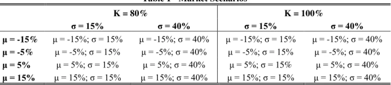
The annualized mean returns presented in Table 2 are given by:
where, is the portfolio strategy average value at maturity, is the initial portfolio investment and T is the number of years of the investment period.
The Table 2 results demonstrate that in the four bear market scenarios, for both floors, all strategies have higher expected returns than the underlying asset and also all the strategies have higher returns with a floor of 100%. This conclusion is justified by the ability of Portfolio Insurance to limit downside risk. Also in the four bear market scenarios, the CPPI 1 strategy has the higher expected returns when the floor is 80%. Then, with a floor of 100%, the CPPI 1 strategy also has the higher expected returns
with the exception of one scenario (μ = -5%; σ = 40%) in which the SLPI strategy has the higher expected return. Another interesting feature of the bear market scenarios is that all strategies, for both floors, have higher expected returns in the scenarios of higher volatility with the exception of the CPPI 1 strategy that remains almost unchanged.
11 this means that if the investor or manager choose an investment with less risk and set the floor in 100%, he obtains higher expected returns in this strategy. In the other strategies there is exactly the opposite, with some exceptions in some strategies that are unchanged or have variations that are not significant.
Table 2 - Annualized Expected Returns
Scenarios
SLPI OBPI CPPI 1 CPPI 3 CPPI 5 Risky
Asset
K=80% K=100% K=80% K=100% K=80% K=100% K=80% K=100% K=80% K=100%
μ=-15%;σ=15% -4,34% 0,02% -4,34% 0,02% -0,44% 1,99% -3,82% 0,28% -4,25% 0,01% -15,00% μ=-15%;σ=40% -2,33% 1,24% -2,86% 0,65% -0,44% 1,99% -3,10% 0,51% -3,19% 0,47% -15,02% μ=-5%;σ=15% -2,21% 0,77% -2,31% 0,65% 1,78% 3,18% -1,62% 1,25% -2,23% 0,68% -4,98% μ=-5%;σ=40% 1,20% 3,76% -0,08% 2,04% 1,79% 3,18% -0,44% 1,78% -0,49% 1,75% -4,95% μ=5%;σ=15% 5,18% 5,76% 4,98% 5,00% 5,00% 5,00% 5,01% 5,02% 4,99% 5,00% 5,03% μ=5%;σ=40% 7,42% 8,74% 5,04% 5,04% 5,01% 4,99% 4,94% 4,99% 4,97% 4,94% 5,01% μ=15%;σ=15% 14,98% 15,00% 14,67% 13,37% 9,38% 7,67% 14,83% 13,48% 14,97% 14,49% 14,99% μ=15%;σ=40% 15,70% 16,31% 12,34% 9,92% 9,37% 7,70% 13,21% 11,28% 13,42% 11,36% 15,11%
Highest values / Lowest values
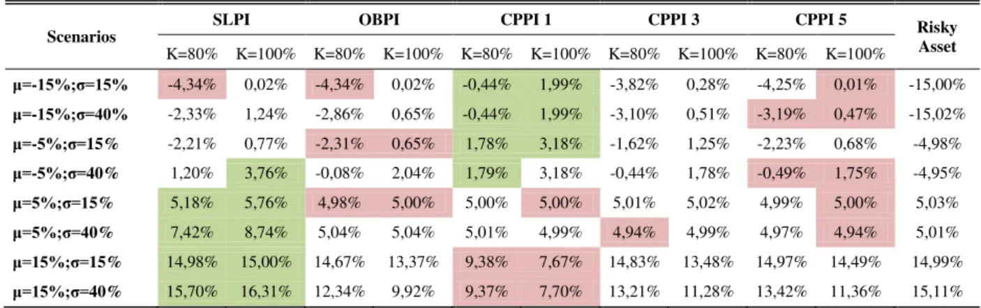
The annualized volatilities (standard deviations) presented in Table 3 are given by:
where STD is the MATLAB function for standard deviation, RT are the five years returns and T is the number of years of the investment period.
The Table 3 results demonstrate, as expected, that in all scenarios the strategies have higher volatility when the underlying risky asset has a volatility of 40%. Another reason for a high volatility in the strategies results in the choice of the 80% floor, with the exception of one case of CPPI 5 strategy in a single scenario (note that in scenario
μ=15%;σ=15%, the volatility of the CPPI 5 strategy is just 15,25%) . Therefore we can state, the more volatile the underlying asset and the smaller the floor required, the higher is the volatility of returns of Portfolio Insurance strategies. In general the strategies have lower volatility compared to the risky asset, with some not significant exceptions, which confirms the effect of limiting the downside risk. Another effect of Portfolio Insurance is the fact that the bullish is the scenario, the higher is the volatility in all strategies for both floors. The CPPI 1 strategy presents the lowest standard deviations for both floors in seven of the eight scenarios, but on the other hand, the SLPI strategy generally has the highest volatility in most scenarios and especially with a floor of 100%.
12 skew has frequent small losses and a few extreme gains and a return distribution with negative skew has frequent small gains and a few extreme losses. Although we do not consider utility function in this study, investors or managers should prefer portfolios that are right-skewed to portfolios that are left-skewed (Harvey and Siddique, 2000).
Table 3 - Annualized Volatilities (Standard Deviations)
Scenarios
SLPI OBPI CPPI 1 CPPI 3 CPPI 5 Risky
Asset
K=80% K=100% K=80% K=100% K=80% K=100% K=80% K=100% K=80% K=100%
μ=-15%;σ=15% 1,63% 0,56% 1,61% 0,55% 2,73% 1,45% 1,80% 0,77% 1,49% 0,47% 14,96% μ=-15%;σ=40% 10,11% 7,61% 8,38% 4,85% 7,17% 3,99% 7,98% 4,58% 8,22% 4,92% 40,06% μ=-5%;σ=15% 7,51% 4,29% 7,24% 3,72% 3,98% 2,21% 6,23% 3,17% 6,96% 3,48% 15,00% μ=-5%;σ=40% 16,85% 13,57% 14,16% 8,89% 10,06% 5,97% 14,27% 9,22% 14,87% 9,85% 40,00% μ=5%;σ=15% 13,65% 11,46% 13,44% 10,23% 5,57% 3,30% 12,81% 9,06% 13,74% 11,03% 15,03% μ=5%;σ=40% 24,51% 21,00% 21,04% 14,39% 13,54% 8,47% 22,50% 16,05% 23,43% 16,93% 40,14% μ=15%;σ=15% 15,00% 14,72% 14,78% 13,50% 7,35% 4,71% 15,28% 14,69% 15,25% 15,76% 14,98% μ=15%;σ=40% 31,30% 28,50% 27,61% 20,24% 17,42% 11,74% 31,21% 24,90% 32,55% 26,29% 40,10%
Highest values / Lowest values
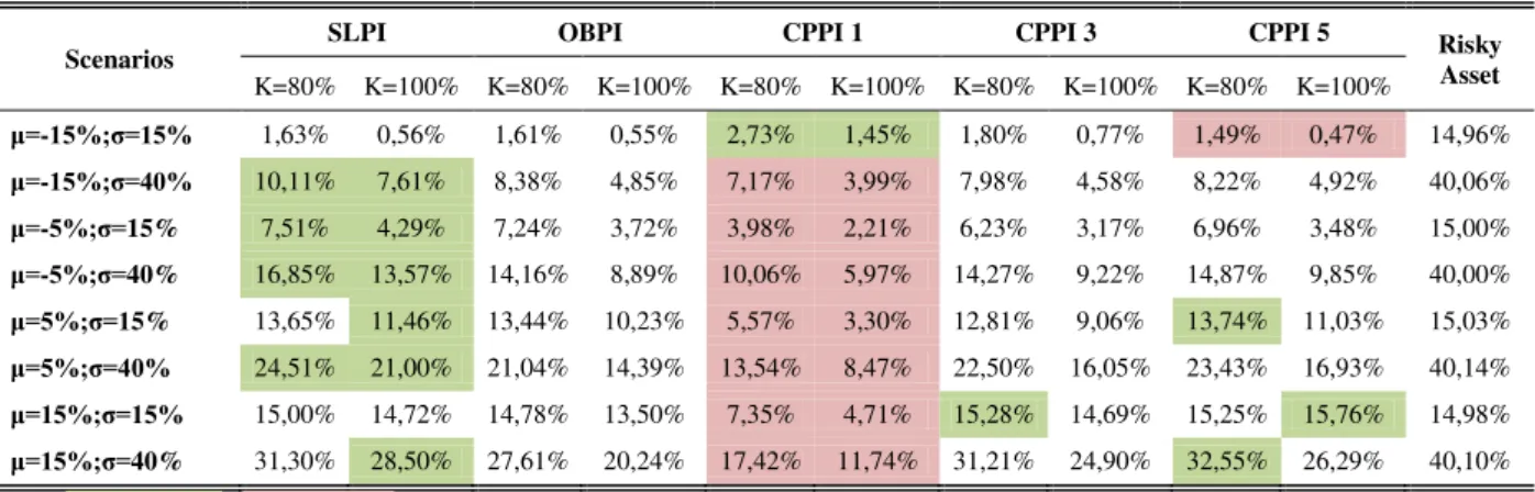
The return distributions of all strategies in all scenarios generally are positively skewed and the effect of choosing a higher floor causes an increase in the skewness. In almost all cases, the scenarios where the underlying asset has more volatility, there is an increase in skewness, for both floors, in the three CPPI strategies, but in the in the remaining no longer applies this standard. There is a tendency on both floors of increased skewness in all strategies as the scenarios become more bear. The strategy CPPI 1 has the lowest coefficient of skewness in the four bear market scenarios for both floors. In general the CPPI 3 and CPPI 5 strategies have the highest values of skewness.
Table 4 - Relative Skewness
Scenarios
SLPI OBPI CPPI 1 CPPI 3 CPPI 5 Risky
Asset
K=80% K=100% K=80% K=100% K=80% K=100% K=80% K=100% K=80% K=100% μ=-15%;σ=15% 8,77 20,11 9,04 21,77 0,83 0,95 4,85 4,88 9,19 22,44 0,01 μ=-15%;σ=40% 4,32 5,51 4,57 6,20 2,29 2,77 6,43 10,79 6,20 10,25 -0,01 μ=-5%;σ=15% 2,06 3,75 2,06 3,84 0,72 0,87 2,40 3,75 2,40 5,08 0,00 μ=-5%;σ=40% 2,54 3,12 2,68 3,76 1,94 2,54 3,58 5,70 3,54 5,63 0,00 μ=5%;σ=15% 0,43 0,93 0,45 0,99 0,63 0,78 0,73 1,61 0,50 1,34 0,00 μ=5%;σ=40% 1,53 1,91 1,66 2,32 1,59 2,07 2,13 3,30 2,07 3,34 0,01 μ=15%;σ=15% 0,01 0,11 0,04 0,17 0,51 0,68 0,02 0,37 0,00 0,10 -0,01 μ=15%;σ=40% 0,88 1,14 1,02 1,48 1,29 1,78 1,21 1,97 1,19 1,98 0,01
Highest values / Lowest values
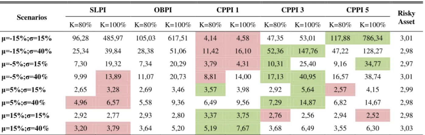
13 returns with large deviations. The return distributions have mostly a leptokurtic behaviour, but there are still some cases where the distributions are considered platykurtic. In most cases the more volatile the underlying asset, the higher is the kurtosis in the three CPPI strategies, in the remaining there is no standard. In most cases the strategies obtain higher kurtosis with a floor of 100%. In general the kurtosis is higher in all strategies, for both floors, as the scenarios become more bear. The CPPI 1 strategy has the lowest coefficients in almost all bear market scenarios and in the normal and bull scenarios is the strategy that has more cases of higher kurtosis. Generally the CPPI 3 strategy has the highest kurtosis and the SLPI strategy presents in some scenarios the lowest coefficients. This leptokurtic and positive-skewed behaviour lead to that most of the strategies have no extreme negative returns and if extreme returns occur it will only be positive.
Table 5 - Relative Kurtosis
Scenarios
SLPI OBPI CPPI 1 CPPI 3 CPPI 5 Risky
Asset
K=80% K=100% K=80% K=100% K=80% K=100% K=80% K=100% K=80% K=100% μ=-15%;σ=15% 96,28 485,97 105,03 617,51 4,14 4,58 47,35 53,01 117,88 786,34 3,01 μ=-15%;σ=40% 25,34 39,84 28,38 51,06 11,42 16,10 52,36 147,76 47,22 128,27 2,98 μ=-5%;σ=15% 7,30 19,32 7,34 20,29 3,79 4,31 10,31 25,40 9,16 34,77 2,97 μ=-5%;σ=40% 9,99 13,89 11,07 20,73 8,81 14,00 17,13 40,95 16,57 38,74 3,01 μ=5%;σ=15% 2,65 3,28 2,69 3,46 3,57 3,98 2,92 5,64 2,57 4,15 2,99 μ=5%;σ=40% 4,96 6,57 5,58 9,36 6,49 9,56 7,29 14,87 6,82 14,67 2,98 μ=15%;σ=15% 2,92 2,77 2,93 2,80 3,37 3,75 2,76 2,56 2,94 2,52 2,98 μ=15%;σ=40% 3,20 3,79 3,64 5,20 5,19 7,67 3,68 6,49 3,55 6,30 3,03
Highest values / Lowest values
4.2
Ratio Analysis
In this subsection we analyze Portfolio Insurance strategies in all scenarios using as performance ratios: Shape ratio, Sortino ratio, Omega ratio and Upside Potential
ratio. The Sharpe ratio (see for example Sharpe (1994)) where is the expected return
on the portfolio, rf is the risk-free interest rate (5%) and is the standard deviation of
returns on the portfolio. The ratio is given by:
The Sharpe ratio can be described as the return per unit of risk. The higher the ratio, the better is the combined performance of risk and return (Bacon, 2008). Although it is a measure commonly used in this theme, in a Portfolio Insurance context this ratio is not necessarily an adequate performance measure, since portfolio insurers do not only care about the mean and variance returns (Annaert et al., 2009).
The Sortino ratio (see for example Sortino and Price (1994)) measures the excess returns over a minimum acceptable return (MAR). The risk in the denominator
14
The Sortino ratio is derived from the Sharpe ratio where volatility is replaced by downside deviation and measures the return per unit of downside risk. Using downside risk the Sortino ratio only penalises return that falls below the MAR. This is an important feature as most investors consider risk as the probability of not achieving their MAR, which means they only fear the downside risk.
The Omega ratio (see for example Shadwick and Keating (2002)) is the expected gain above the MAR value divided by the expected loss below the MAR and where [a,b] is the interval of returns with a cumulative distribution function F(x). This ratio is defined by:
The Omega ratio is defined as the probability weighted ratio of gains to losses relative to a return threshold, in a way that splits the return into two sub-parts according to a minimum accepted return (MAR). The positive returns for the investor or manager are above this MAR and the negative returns below. The investor or manager should always prefer the portfolio with the highest value of Omega (Bertrand and Prigent, 2011). The main advantage of the Omega measure is that it involves all the moments of the return distribution, including skewness and kurtosis (Bacmann and Scholz, 2003).
The Upside Potential ratio (see for example Sortino et al. (1999)) measures the average returns above the MAR in relation to the downside deviation, as the Sortino Ratio. This ratio is defined by:
The Upside Potential ratio is an alternative of Sortino ratio in way that is the probability weighted average returns above the MAR and considers portfolio risk as downside deviation, penalizing the volatility below the MAR. An important advantage of using this ratio rather than Sortino ratio is the consistency in the use of the MAR for evaluating both profits and losses (Plantinga and Groot, 2001).
In the literature there is not an optimal value for the MAR, however since we are analyzing strategies with guaranteed return we have decided to use the risk-free interest rate of 5% as MAR (see for example Khuman and Constantinou (2009)). Another common value used by the authors is 0%, which would lead to the inability to analyze the strategies with a floor of 100% since they do not have negative returns.
15 volatility, standing incorrectly as being the best portfolio performance. For this reason, in scenarios where these ratios are negative we only analyze those results with Omega and Upside Potential ratios.
In Tables 6, 7, 8 and 9 are presented the Sharpe, Sortino, Omega and Upside Potential ratios, respectively.
In Table 6 are presented the Sharpe ratio results and as mentioned before we only analyzed the positive ratios. Thus, relying only on the four normal and bull market scenarios, the best strategy is the SLPI according to this ratio. On the other hand the worst strategy is the CPPI 1 strategy. Another important result is that the SLPI strategy is the single one to have better results with a floor of 100%, in contrast to all others.
Table 6 –Sharpe Ratios
Scenarios
SLPI OBPI CPPI 1 CPPI 3 CPPI 5 Risky
Asset
K=80% K=100% K=80% K=100% K=80% K=100% K=80% K=100% K=80% K=100% μ=-15%;σ=15% -5,73 -8,89 -5,80 -9,05 -1,99 -2,08 -4,90 -6,13 -6,21 -10,62 -1,34 μ=-15%;σ=40% -0,73 -0,49 -0,94 -0,90 -0,76 -0,75 -1,02 -0,98 -1,00 -0,92 -0,50 μ=-5%;σ=15% -0,96 -0,99 -1,01 -1,17 -0,81 -0,82 -1,06 -1,18 -1,04 -1,24 -0,67 μ=-5%;σ=40% -0,23 -0,09 -0,36 -0,33 -0,32 -0,30 -0,38 -0,35 -0,37 -0,33 -0,25 μ=5%;σ=15% 0,01 0,07 0,00 0,00 0,00 0,00 0,00 0,00 0,00 0,00 0,00 μ=5%;σ=40% 0,10 0,18 0,00 0,00 0,00 0,00 0,00 0,00 0,00 0,00 0,00 μ=15%;σ=15% 0,67 0,68 0,65 0,62 0,60 0,57 0,64 0,58 0,65 0,60 0,67 μ=15%;σ=40% 0,34 0,40 0,27 0,24 0,25 0,23 0,26 0,25 0,26 0,24 0,25
Highest values / Lowest values
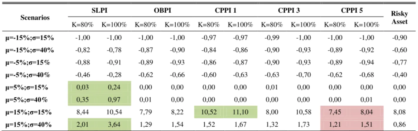
In Table 7 are presented the Sortino ratios and as the Sharpe ratios we only analyze the four normal and bull market scenarios because the other four have negative excess returns. The SLPI strategy has the best performance in three of the four normal and bull analyzed scenarios, whereas in the remainder is the CPPI 1 strategy that has the best performance. On the other hand, the CPPI 5 has the worst performance. In all scenarios analyzed, all the strategies have better ratios with a floor of 100%.
Table 7 –Sortino Ratios
Scenarios
SLPI OBPI CPPI 1 CPPI 3 CPPI 5 Risky
Asset
K=80% K=100% K=80% K=100% K=80% K=100% K=80% K=100% K=80% K=100% μ=-15%;σ=15% -1,00 -1,00 -1,00 -1,00 -0,97 -0,97 -0,99 -1,00 -1,00 -1,00 -0,90 μ=-15%;σ=40% -0,82 -0,78 -0,87 -0,90 -0,84 -0,86 -0,90 -0,93 -0,89 -0,92 -0,60 μ=-5%;σ=15% -0,88 -0,91 -0,89 -0,93 -0,86 -0,87 -0,90 -0,93 -0,89 -0,94 -0,77 μ=-5%;σ=40% -0,46 -0,28 -0,62 -0,66 -0,60 -0,63 -0,63 -0,70 -0,62 -0,68 -0,40 μ=5%;σ=15% 0,03 0,24 0,00 0,00 0,00 0,00 0,01 0,00 0,00 0,00 0,00 μ=5%;σ=40% 0,35 0,97 0,01 0,00 0,00 0,00 0,00 0,00 0,00 0,01 0,00 μ=15%;σ=15% 8,44 10,54 7,79 8,22 10,52 11,10 8,00 10,58 7,45 8,04 8,08 μ=15%;σ=40% 2,01 3,64 1,29 1,54 1,52 1,67 1,32 1,73 1,21 1,51 0,86
Highest values / Lowest values
In Table 8 are presented the Omega ratio results and in the first scenario (µ =
16 zero. Still, in all other scenarios and according to this ratio, the best strategies are the SLPI strategy and the CPPI 1 strategy. The SLPI strategy with a floor of 100% has the best ratio in six scenarios and with a floor of 80%, in three scenarios. The CPPI 1 strategy with a floor of 100% has the best ratio in three scenarios and one scenario with 80% of floor. The CPPI 5 in general has the worst ratios of all strategies, particularly in normal and bull market scenarios. This is an interesting result as it shows high multipliers do not necessarily imply good performance, even when the underlying asset increases. The SLPI in bear market scenarios is the best strategy according to Omega ratio. In most cases the strategies have better ratios for a floor of 100%.
Table 8 –Omega Ratios
Scenarios
SLPI OBPI CPPI 1 CPPI 3 CPPI 5 Risky
Asset
K=80% K=100% K=80% K=100% K=80% K=100% K=80% K=100% K=80% K=100% μ=-15%;σ=15% 0,00 0,00 0,00 0,00 0,00 0,00 0,00 0,00 0,00 0,00 0,00 μ=-15%;σ=40% 0,05 0,10 0,03 0,04 0,04 0,04 0,03 0,03 0,03 0,03 0,02 μ=-5%;σ=15% 0,02 0,03 0,02 0,02 0,02 0,02 0,02 0,02 0,02 0,02 0,01 μ=-5%;σ=40% 0,20 0,36 0,14 0,16 0,15 0,18 0,12 0,13 0,13 0,14 0,08 μ=5%;σ=15% 0,73 1,02 0,68 0,75 0,86 0,91 0,70 0,74 0,68 0,71 0,65 μ=5%;σ=40% 0,71 1,23 0,49 0,59 0,63 0,76 0,43 0,47 0,43 0,45 0,32 μ=15%;σ=15% 32,09 37,60 30,46 27,75 42,01 45,83 26,33 28,54 27,31 21,02 31,09 μ=15%;σ=40% 2,43 4,08 1,72 2,04 2,54 3,01 1,43 1,60 1,28 1,34 1,33
Highest values / Lowest values
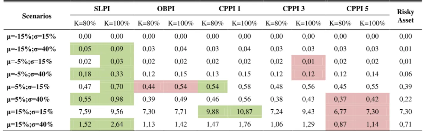
In Table 9 are presented the Upside Potential ratio results and as in the Omega ratios results, in the first scenario (µ = -15%; = 15%) is difficult to choose a strategy since they have values very close to zero. The SLPI strategy has the best ratios in almost all scenarios and remaining scenarios that SLPI strategy is not the best, the CPPI 1 is. Generally the CPPI 5 has the worst ratios, especially in normal and bull market scenarios, the SLPI strategy has the best ratios in bear market scenarios and in more volatile scenarios ( = 40%) for both floors. All the strategies have better ratios in all scenarios when the floor is 100%.
Table 9 –Upside Potential Ratios
Scenarios
SLPI OBPI CPPI 1 CPPI 3 CPPI 5 Risky
Asset
K=80% K=100% K=80% K=100% K=80% K=100% K=80% K=100% K=80% K=100% μ=-15%;σ=15% 0,00 0,00 0,00 0,00 0,00 0,00 0,00 0,00 0,00 0,00 0,00 μ=-15%;σ=40% 0,05 0,09 0,03 0,04 0,03 0,04 0,03 0,03 0,03 0,03 0,01 μ=-5%;σ=15% 0,02 0,03 0,02 0,02 0,02 0,02 0,02 0,01 0,02 0,02 0,01 μ=-5%;σ=40% 0,18 0,33 0,12 0,15 0,13 0,15 0,12 0,12 0,12 0,14 0,06 μ=5%;σ=15% 0,47 0,70 0,44 0,54 0,54 0,58 0,48 0,56 0,45 0,55 0,39 μ=5%;σ=40% 0,55 0,98 0,39 0,49 0,46 0,56 0,38 0,43 0,37 0,42 0,22 μ=15%;σ=15% 7,59 9,56 7,30 7,71 9,88 10,87 7,24 9,43 6,77 7,30 7,30 μ=15%;σ=40% 1,52 2,64 1,13 1,42 1,47 1,76 1,06 1,29 0,87 1,14 0,71
17
4.3
Other Measures
In this section we present further results that help to compare the Portfolio Insurance strategies. These results are based on probabilities of portfolio values to achieve or not certain results.
Table 10 presents the probability of each strategy reaching a portfolio value no higher than the floor value plus 5% at the end of each year, during an investment period of five years, for both floors. The probability is obtained each year by the number of times (100.000 simulations) that the portfolio value is not higher than the floor (K) on that year, discounted at the risk-free interest rate, plus 5%. The purpose of adding to this calculation the 5% is to be able to study the different strategies whether they have a portfolio value close to the value of the floor, since the CPPI strategies never are fully invested in risk-free assets, that is, never “touch” the floor barrier, and is that what could happen with the SLPI and OBPI strategies.
Obviously, all strategies in all scenarios, have higher probability of having a value below the floor barrier (K+5%), when they have a floor of 100%. Also, in most cases, the probabilities of all strategies also increase when the scenarios are more volatile.
The strategy CPPI 5 is the one with a higher probability in the eight scenarios when the portfolio has a floor of 100%. For a floor of 80%, the CPPI 5 has the highest
probability in scenarios where the volatility is = 40%. In the all four scenarios which have a lower volatility ( = 15%), the SLPI and OBPI strategy have the highest probabilities when the floor is 80%. The CPPI 1 strategy has the lowest probabilities in all scenarios for both floors.
Table 11 presents the probability of each strategy has a portfolio value higher than a portfolio fully invested in risk-free assets with an interest rate of 5% per year, during an investment period of five years, for both floors. The probability is obtained each year by the number of times (100.000 simulations) that the portfolio value of each strategy is higher than a portfolio that is rewarded by 5% at the end of each year. The aim of this probability is to know if the Portfolio Insurance strategies are a better investment and achieve a superior portfolio value in different market conditions than an investment without risk, for example in government bonds.
18 OBPI, CPPI 3 and CPPI 5 strategies to be higher than the portfolio value invested in risk-free assets. The strategies with a floor of 80% have always higher probabilities than a floor of 100% and the volatility of 40% in bear market scenarios increases the probabilities while in normal and bull market scenarios has the opposite effect.
Table 10 - Probability to have the portfolio value ≤ K + 5% during the investment period
μ=-15%;σ=15% K 1 2 3 4 5 μ=5%;σ=15% K 1 2 3 4 5
SLPI 80% 8% 50% 79% 92% 97% SLPI 80% 0% 3% 7% 10% 14%
100% 53% 85% 95% 98% 99% 100% 10% 20% 26% 30% 33%
OBPI 80% 0% 21% 63% 88% 97% OBPI 80% 0% 0% 2% 7% 14%
100% 12% 64% 90% 98% 99% 100% 1% 6% 15% 25% 34%
CPPI 1 80% 0% 0% 0% 0% 0% CPPI 1 80% 0% 0% 0% 0% 0%
100% 0% 0% 0% 0% 2% 100% 0% 0% 0% 0% 0%
CPPI 3 80% 0% 4% 30% 62% 83% CPPI 3 80% 0% 0% 0% 1% 6%
100% 1% 30% 68% 88% 96% 100% 0% 1% 3% 7% 11%
CPPI 5 80% 1% 32% 69% 89% 96% CPPI 5 80% 0% 1% 4% 7% 11%
100% 26% 76% 93% 98% 100% 100% 2% 12% 21% 29% 36%
μ=-15%;σ=40% K 1 2 3 4 5 μ=5%;σ=40% K 1 2 3 4 5
SLPI 80% 36% 59% 73% 81% 86% SLPI 80% 20% 32% 39% 45% 49%
100% 58% 74% 82% 87% 91% 100% 38% 47% 52% 56% 59%
OBPI 80% 2% 22% 48% 71% 87% OBPI 80% 1% 7% 19% 32% 50%
100% 12% 44% 68% 82% 92% 100% 5% 20% 34% 47% 61%
CPPI 1 80% 0% 0% 1% 4% 11% CPPI 1 80% 0% 0% 0% 0% 1%
100% 0% 2% 10% 22% 36% 100% 0% 0% 2% 4% 7%
CPPI 3 80% 15% 49% 71% 82% 89% CPPI 3 80% 6% 23% 38% 48% 57%
100% 36% 70% 85% 92% 95% 100% 20% 40% 56% 65% 74%
CPPI 5 80% 37% 69% 83% 90% 94% CPPI 5 80% 21% 42% 55% 64% 70%
100% 26% 86% 93% 96% 98% 100% 47% 66% 75% 81% 84%
μ=-5%;σ=15% K 1 2 3 4 5 μ=15%;σ=15% K 1 2 3 4 5
SLPI 80% 2% 17% 36% 53% 65% SLPI 80% 0% 0% 0% 0% 0%
100% 28% 54% 69% 79% 86% 100% 3% 4% 4% 3% 3%
OBPI 80% 0% 4% 21% 44% 66% OBPI 80% 0% 0% 0% 0% 0%
100% 3% 28% 55% 74% 86% 100% 0% 1% 1% 2% 3%
CPPI 1 80% 0% 0% 0% 0% 0% CPPI 1 80% 0% 0% 0% 0% 0%
100% 0% 0% 0% 0% 0% 100% 0% 0% 0% 0% 0%
CPPI 3 80% 0% 0% 5% 15% 30% CPPI 3 80% 0% 0% 0% 0% 0%
100% 0% 7% 25% 44% 61% 100% 0% 0% 0% 0% 0%
CPPI 5 80% 0% 8% 26% 45% 61% CPPI 5 80% 0% 0% 0% 0% 0%
100% 10% 40% 64% 78% 87% 100% 0% 2% 2% 3% 3%
μ=-5%;σ=40% K 1 2 3 4 5 μ=15%;σ=40% K 1 2 3 4 5
SLPI 80% 27% 45% 57% 65% 70% SLPI 80% 13% 21% 24% 27% 28%
100% 48% 61% 69% 74% 78% 100% 29% 34% 35% 36% 37%
OBPI 80% 1% 13% 32% 52% 71% OBPI 80% 0% 3% 9% 17% 29%
100% 8% 31% 50% 66% 80% 100% 3% 11% 20% 29% 39%
CPPI 1 80% 0% 0% 0% 1% 4% CPPI 1 80% 0% 0% 0% 0% 0%
100% 0% 1% 4% 10% 18% 100% 0% 0% 0% 1% 2%
CPPI 3 80% 10% 35% 54% 67% 76% CPPI 3 80% 4% 14% 23% 29% 35%
100% 0% 56% 72% 81% 87% 100% 13% 29% 39% 46% 51%
CPPI 5 80% 28% 56% 70% 79% 85% CPPI 5 80% 14% 30% 39% 45% 51%
100% 56% 77% 86% 90% 93% 100% 37% 53% 61% 66% 69%
19
Table 11 - Probability to have the portfolio value > 5% risk-free investment
μ=-15%;σ=15% K 1 2 3 4 5 μ=5%;σ=15% K 1 2 3 4 5
SLPI 80% 8% 2% 1% 0% 0% SLPI 80% 47% 46% 45% 44% 43%
100% 8% 2% 1% 0% 0% 100% 47% 45% 45% 44% 43%
OBPI 80% 8% 2% 1% 0% 0% OBPI 80% 46% 44% 43% 43% 42%
100% 7% 2% 1% 0% 0% 100% 44% 42% 40% 39% 39%
CPPI 1 80% 8% 2% 1% 0% 0% CPPI 1 80% 47% 46% 45% 44% 43%
100% 8% 2% 1% 0% 0% 100% 47% 46% 45% 44% 43%
CPPI 3 80% 8% 2% 1% 0% 0% CPPI 3 80% 46% 44% 42% 41% 35%
100% 6% 1% 0% 0% 0% 100% 41% 38% 35% 33% 32%
CPPI 5 80% 8% 2% 1% 0% 0% CPPI 5 80% 47% 45% 45% 44% 42%
100% 7% 2% 0% 0% 0% 100% 44% 40% 37% 35% 33%
μ=-15%;σ=40% K 1 2 3 4 5 μ=5%;σ=40% K 1 2 3 4 5
SLPI 80% 24% 16% 11% 8% 6% SLPI 80% 42% 39% 36% 35% 33%
100% 24% 16% 11% 8% 6% 100% 42% 39% 36% 35% 33%
OBPI 80% 22% 14% 9% 6% 4% OBPI 80% 39% 35% 32% 30% 28%
100% 21% 13% 8% 5% 4% 100% 39% 34% 30% 27% 25%
CPPI 1 80% 24% 16% 11% 8% 6% CPPI 1 80% 42% 39% 36% 34% 33%
100% 24% 16% 11% 8% 6% 100% 42% 39% 36% 35% 32%
CPPI 3 80% 21% 12% 7% 5% 3% CPPI 3 80% 37% 32% 27% 24% 21%
100% 15% 7% 4% 3% 2% 100% 29% 24% 19% 17% 15%
CPPI 5 80% 23% 13% 8% 5% 3% CPPI 5 80% 40% 34% 29% 25% 22%
100% 7% 8% 4% 3% 2% 100% 30% 23% 19% 15% 13%
μ=-5%;σ=15% K 1 2 3 4 5 μ=15%;σ=15% K 1 2 3 4 5
SLPI 80% 23% 15% 10% 7% 5% SLPI 80% 72% 80% 85% 88% 91%
100% 23% 15% 10% 7% 5% 100% 72% 80% 85% 88% 91%
OBPI 80% 22% 14% 9% 6% 5% OBPI 80% 71% 79% 84% 87% 90%
100% 21% 13% 8% 5% 4% 100% 70% 77% 82% 86% 89%
CPPI 1 80% 23% 15% 10% 7% 5% CPPI 1 80% 72% 80% 85% 88% 91%
100% 23% 15% 10% 7% 5% 100% 72% 80% 85% 88% 91%
CPPI 3 80% 22% 14% 9% 6% 4% CPPI 3 80% 72% 79% 83% 86% 89%
100% 19% 11% 6% 4% 2% 100% 67% 73% 78% 82% 85%
CPPI 5 80% 23% 15% 10% 7% 5% CPPI 5 80% 72% 80% 84% 88% 90%
100% 20% 12% 7% 5% 3% 100% 69% 75% 79% 82% 85%
μ=-5%;σ=40% K 1 2 3 4 5 μ=15%;σ=40% K 1 2 3 4 5
SLPI 80% 32% 26% 22% 18% 16% SLPI 80% 52% 53% 53% 54% 55%
100% 33% 26% 22% 18% 16% 100% 52% 53% 54% 54% 54%
OBPI 80% 30% 23% 18% 15% 13% OBPI 80% 49% 49% 48% 48% 49%
100% 29% 22% 17% 13% 11% 100% 48% 47% 47% 46% 46%
CPPI 1 80% 33% 26% 21% 18% 16% CPPI 1 80% 52% 53% 53% 54% 55%
100% 33% 26% 22% 18% 16% 100% 52% 53% 54% 54% 54%
CPPI 3 80% 28% 20% 15% 12% 9% CPPI 3 80% 47% 45% 43% 42% 40%
100% 19% 14% 10% 7% 5% 100% 38% 35% 33% 31% 30%
CPPI 5 80% 31% 23% 17% 13% 10% CPPI 5 80% 50% 47% 45% 42% 40%
100% 22% 14% 10% 7% 5% 100% 39% 34% 31% 28% 26%
20
4.4
Stochastic Dominance
The stochastic dominance is a basic concept of decision theory. The decision rule for first order stochastic dominance was introduced by Quirk and Saposnik (1962) which is related to the investors‟ preferences. The first order is also the strongest criteria which implies second and third order stochastic dominance (Zagst and Kraus, 2011) and says that a random variable A stochastically dominates a random variable B at the first order if and only if the cumulative distribution function of A, denoted by FA, is always below the cumulative distribution FB of B (see for example Bertrand and Prigent (2005)). For investments, it means that if an investment strategy stochastically dominates another, all investors that prefer more to less would always prefer the dominant strategy. The second order states that A dominates B if the sum of the cumulative distribution of A is always below of the sum of the cumulative distribution of B. For the investor, if a strategy dominates another on the second order, it means that every investor who is risk averse, prefer the dominant strategy. The third order of dominance says that A dominates B if the sum of the sum of the cumulative distribution of A is always below of the sum of the sum of the cumulative distribution B (see for example Zagst and Kraus (2011)). The investors who have decreasing risk aversion with respect to wealth, will always prefer a strategy that dominates stochastically another on third order.
Hence we compute the cumulative distribution, the sum of cumulative distribution and the sum of the sum of cumulative distribution functions of returns of the five strategies in the eight scenarios for both floors. These distributions are illustrated in Appendix B, see Figures B.1, B.2 and B.3 with a floor of 80% and in Figures B.4, B.5 and B.6 with a floor of 100%.
The Table 12, 13 and 14 presents the results for stochastic dominance on first order, second order and third order, respectively. In the table the number „1‟ means that the strategy on the left column dominates the correspondent in the upper row.
On the first order of dominance there are eight cases where investors or managers always prefer the SLPI strategy to OBPI strategy. This situation occurs with a floor of 80% in three scenarios and with a floor of 100% in five scenarios.
On the second order of dominance the investors who are risk averse always prefer the CPPI 1 strategy in all bear market scenarios, since the CPPI 1 strategy dominates all the other strategies in these four bear market scenarios for both floors. In bull market scenarios the CPPI 1 also dominates in some cases, particularly in relation to CPPI 3 and CPPI 5 strategies. However we could not state that investors or managers who are risk averse always prefer the CPPI 1 strategy in bull market scenarios.
21 managers who have decreasing risk aversion with respect to wealth always prefer the CPPI 1 strategy in bear markets scenarios, as in the previous order, and also in one normal market bull scenario (μ = 5%, σ = 15%) for both floors.
22
Table 12 - Stochastic Dominance - First Order
K=80% K=100%
μ=-15%;σ=15% SLPI OBPI CPPI 1 CPPI 3 CPPI 5 μ=-15%;σ=15% SLPI OBPI CPPI 1 CPPI 3 CPPI 5
SLPI 0 0 0 0 SLPI 0 0 0 0
OBPI 0 0 0 0 OBPI 0 0 0 0
CPPI 1 0 0 0 0 CPPI 1 0 0 0 0
CPPI 3 0 0 0 0 CPPI 3 0 0 0 0
CPPI 5 0 0 0 0 CPPI 5 0 0 0 0
μ=-15%;σ=40% SLPI OBPI CPPI 1 CPPI 3 CPPI 5 μ=-15%;σ=40% SLPI OBPI CPPI 1 CPPI 3 CPPI 5
SLPI 1 0 0 0 SLPI 0 0 0 0
OBPI 0 0 0 0 OBPI 0 0 0 0
CPPI 1 0 0 0 0 CPPI 1 0 0 0 0
CPPI 3 0 0 0 0 CPPI 3 0 0 0 0
CPPI 5 0 0 0 0 CPPI 5 0 0 0 0
μ=-5%;σ=15% SLPI OBPI CPPI 1 CPPI 3 CPPI 5 μ=-5%;σ=15% SLPI OBPI CPPI 1 CPPI 3 CPPI 5
SLPI 0 0 0 0 SLPI 0 0 0 0
OBPI 0 0 0 0 OBPI 0 0 0 0
CPPI 1 0 0 0 0 CPPI 1 0 0 0 0
CPPI 3 0 0 0 0 CPPI 3 0 0 0 0
CPPI 5 0 0 0 0 CPPI 5 0 0 0 0
μ=-5%;σ=40% SLPI OBPI CPPI 1 CPPI 3 CPPI 5 μ=-5%;σ=40% SLPI OBPI CPPI 1 CPPI 3 CPPI 5
SLPI 0 0 0 0 SLPI 1 0 0 0
OBPI 0 0 0 0 OBPI 0 0 0 0
CPPI 1 0 0 0 0 CPPI 1 0 0 0 0
CPPI 3 0 0 0 0 CPPI 3 0 0 0 0
CPPI 5 0 0 0 0 CPPI 5 0 0 0 0
μ=5%;σ=15% SLPI OBPI CPPI 1 CPPI 3 CPPI 5 μ=5%;σ=15% SLPI OBPI CPPI 1 CPPI 3 CPPI 5
SLPI 0 0 0 0 SLPI 0 0 0 0
OBPI 0 0 0 0 OBPI 0 0 0 0
CPPI 1 0 0 0 0 CPPI 1 0 0 0 0
CPPI 3 0 0 0 0 CPPI 3 0 0 0 0
CPPI 5 0 0 0 0 CPPI 5 0 0 0 0
μ=5%;σ=40% SLPI OBPI CPPI 1 CPPI 3 CPPI 5 μ=5%;σ=40% SLPI OBPI CPPI 1 CPPI 3 CPPI 5
SLPI 0 0 0 0 SLPI 1 0 0 0
OBPI 0 0 0 0 OBPI 0 0 0 0
CPPI 1 0 0 0 0 CPPI 1 0 0 0 0
CPPI 3 0 0 0 0 CPPI 3 0 0 0 0
CPPI 5 0 0 0 0 CPPI 5 0 0 0 0
μ=15%;σ=15% SLPI OBPI CPPI 1 CPPI 3 CPPI 5 μ=15%;σ=15% SLPI OBPI CPPI 1 CPPI 3 CPPI 5
SLPI 0 0 0 0 SLPI 0 0 0 0
OBPI 0 0 0 0 OBPI 0 0 0 0
CPPI 1 0 0 0 0 CPPI 1 0 0 0 0
CPPI 3 0 0 0 0 CPPI 3 0 0 0 0
CPPI 5 0 0 0 0 CPPI 5 0 0 0 0
μ=15%;σ=40% SLPI OBPI CPPI 1 CPPI 3 CPPI 5 μ=15%;σ=40% SLPI OBPI CPPI 1 CPPI 3 CPPI 5
SLPI 0 0 0 0 SLPI 0 0 0 0
OBPI 0 0 0 0 OBPI 0 0 0 0
CPPI 1 0 0 0 0 CPPI 1 0 0 0 0
CPPI 3 0 0 0 0 CPPI 3 0 0 0 0
23
Table 13 - Stochastic Dominance - Second Order
K=80% K=100%
μ=-15%;σ=15% SLPI OBPI CPPI 1 CPPI 3 CPPI 5 μ=-15%;σ=15% SLPI OBPI CPPI 1 CPPI 3 CPPI 5
SLPI 1 0 0 0 SLPI 0 0 0 0
OBPI 0 0 0 0 OBPI 0 0 0 0
CPPI 1 1 1 1 1 CPPI 1 1 1 1 1
CPPI 3 1 1 0 1 CPPI 3 1 1 0 1
CPPI 5 1 1 0 0 CPPI 5 1 1 0 0
μ=-15%;σ=40% SLPI OBPI CPPI 1 CPPI 3 CPPI 5 μ=-15%;σ=40% SLPI OBPI CPPI 1 CPPI 3 CPPI 5
SLPI 1 0 0 1 SLPI 1 0 0 0
OBPI 0 0 0 1 OBPI 0 0 0 0
CPPI 1 1 1 1 1 CPPI 1 1 1 1 1
CPPI 3 0 0 0 1 CPPI 3 0 1 0 1
CPPI 5 0 0 0 0 CPPI 5 0 1 0 0
μ=-5%;σ=15% SLPI OBPI CPPI 1 CPPI 3 CPPI 5 μ=-5%;σ=15% SLPI OBPI CPPI 1 CPPI 3 CPPI 5
SLPI 0 0 0 0 SLPI 0 0 0 0
OBPI 0 0 0 0 OBPI 0 0 0 0
CPPI 1 1 1 1 1 CPPI 1 1 1 1 1
CPPI 3 1 1 0 1 CPPI 3 1 1 0 1
CPPI 5 0 0 0 0 CPPI 5 1 1 0 0
μ=-5%;σ=40% SLPI OBPI CPPI 1 CPPI 3 CPPI 5 μ=-5%;σ=40% SLPI OBPI CPPI 1 CPPI 3 CPPI 5
SLPI 1 0 0 1 SLPI 1 0 0 0
OBPI 0 0 0 1 OBPI 0 0 0 0
CPPI 1 1 1 1 1 CPPI 1 1 1 1 1
CPPI 3 0 0 0 1 CPPI 3 0 0 0 1
CPPI 5 0 0 0 0 CPPI 5 0 0 0 0
μ=5%;σ=15% SLPI OBPI CPPI 1 CPPI 3 CPPI 5 μ=5%;σ=15% SLPI OBPI CPPI 1 CPPI 3 CPPI 5
SLPI 0 0 0 0 SLPI 1 0 0 0
OBPI 0 0 0 0 OBPI 0 0 0 0
CPPI 1 1 1 1 1 CPPI 1 0 1 1 1
CPPI 3 0 1 0 1 CPPI 3 0 1 0 1
CPPI 5 0 0 0 0 CPPI 5 0 0 0 0
μ=5%;σ=40% SLPI OBPI CPPI 1 CPPI 3 CPPI 5 μ=5%;σ=40% SLPI OBPI CPPI 1 CPPI 3 CPPI 5
SLPI 0 0 0 1 SLPI 1 0 0 0
OBPI 0 0 0 1 OBPI 0 0 0 0
CPPI 1 1 1 1 1 CPPI 1 0 1 1 1
CPPI 3 0 0 0 1 CPPI 3 0 0 0 1
CPPI 5 0 0 0 0 CPPI 5 0 0 0 0
μ=15%;σ=15% SLPI OBPI CPPI 1 CPPI 3 CPPI 5 μ=15%;σ=15% SLPI OBPI CPPI 1 CPPI 3 CPPI 5
SLPI 1 0 0 0 SLPI 0 0 0 0
OBPI 0 0 0 0 OBPI 0 0 0 0
CPPI 1 0 0 0 0 CPPI 1 0 0 0 0
CPPI 3 0 0 0 0 CPPI 3 0 0 0 0
CPPI 5 0 0 0 0 CPPI 5 0 0 0 0
μ=15%;σ=40% SLPI OBPI CPPI 1 CPPI 3 CPPI 5 μ=15%;σ=40% SLPI OBPI CPPI 1 CPPI 3 CPPI 5
SLPI 1 0 0 1 SLPI 1 0 0 0
OBPI 0 0 0 1 OBPI 0 0 0 0
CPPI 1 0 0 1 1 CPPI 1 0 0 1 1
CPPI 3 0 0 0 1 CPPI 3 0 0 0 1