Carlos Pestana Barros & Nicolas Peypoch
A Comparative Analysis of Productivity Change in Italian and
Portuguese Airports
WP 006/2007/DE
_________________________________________________________
Felipa de Mello-Sampayo and Sofia de Sousa-Vale
Tourism and Growth in European Countries:
An Application of
Likelihood-Based Panel Cointegration*
WP 17/2012/DE
_________________________________________________________
De pa rtme nt o f Ec o no mic s
W
ORKINGP
APERSISSN Nº 0874-4548
School of Economics and Management
Tourism and Growth in European Countries: An Application of
Likelihood-Based Panel Cointegration
∗Felipa de Mello-Sampayo† and Sofia de Sousa-Vale†
†
ISCTE–IUL Institute University of Lisbon
Abstract
This paper applies likelihood-based panel cointegration techniques to examine the exis-tence of a long run relationship between GDP, tourism earnings per tourist and total trade volume for a panel of European countries over the period 1988–2010. Removing the cross dependency, our panel tourism-led growth model indicates that tourism development has a higher impact on GDP in the North than in South European countries. The policy impli-cation of this result is that for this group of countries, the best strategy is to raise tourism receipts. Furthermore, the volume of trade shows a significant and much more stronger effect on the long run economic growth in our sample economies than tourism does.
JEL Classification: F43; C33; L83
Keywords: Tourism; Economic growth; Rank tests; Panel unit root tests; Panel cointegration
Postal address: ISCTE-IUL, Department of Economics, Av. For¸cas Armadas, 1649–026, Lisbon, Portugal.
Author’s email: [email protected]
∗We are grateful to Francisco Camoes, anonymous referees and to the participants at the 5th
Portuguese Economic Journal Conference, 4th
CSDA International Conference on Computational and Financial Econometrics (CFE 10), 3rd
1
Introduction
As globalization reaches the remotest economies in the world, international tourism has been steadily increasing, as well as the importance of the tourism industry for the economy of many countries. According to the World Travel & Tourism Council (WTTC)1, Tourism was a major source of economic growth to European countries, especially in small countries such as Malta, where it averaged 11% of Gross Domestic Product (GDP) in 2008 but also in larger countries such as Spain where the tourism sector amounted to 6.1% in the same period. Tourism-generated proceeds have come to represent an increasing employment, external revenue source, household income and government income. Thus, tourism plays, nowadays, a key role in boosting the countries’ economies.
In the literature on growth, the export-led growth hypothesis (see McKinnon, 1964) postu-lates that international tourism contributes to growth in two ways. In the first place, enhancing efficiency through competition between the local sectors and foreign destinations (Bhagwati and Srinivasan, 1979, Krueger, 1980). Secondly, by facilitating the exploitation of economies of scale in local firms (Helpman and Krugman, 1985). On the other hand, there are economic, social and environmental costs associated with tourism activity (Palmer and Riera, 2003). If the negative externalities from tourism activity outweigh its benefits, the development of tourism activity may turn out to deter economic growth.
The growing importance of tourism on the national economies led to the emergence of the Tourism Satellite Account2 (TSA) worldwide that provides a means of separating and examin-ing both tourism supply and tourism demand within the general framework of the System of National Accounts and, simultaneously, important contributions have been made to estimate empirically different forms and degrees of tourism on long-run economic growth (see Balaguer and Cantavella-Jord´a, 2002, Eugenio-Martin, 2004, Oh, 2005, Gunduz and Hatemi-J., 2005, Lee and Chang, 2008, Katircioglu, 2009, Cort´es-Jimen´ez and Pulina, 2010).
The branch of empirical research on the effects of tourism on economic growth that focuses on a single country and cointegrates gross domestic product (GDP) with the number of tourist arrivals (or alternatively with the volume of tourism receipts) and real exchange rate3 has found
that tourism has generally a positive impact on economic growth. Balaguer and Cantavella-Jord´a (2002) tested the tourism-led growth hypothesis for Spain through cointegration and causality tests relating real GDP, international tourism earnings and the real effective exchange rate, confirming the existence of a stable relationship between economic growth and tourism. They also found causality from tourism activity to economic growth. Gunduz and Hatemi-J. (2005) tested the tourism-led growth hypothesis for Turkey applying a causality test based on leverage bootstrap simulations between the number of tourist arrivals, real gross domestic product and real exchange rates. They support empirically the tourism-led growth hypothesis. Katircioglu (2009) used cointegration and Granger causality tests to analyze the existence of a long-run equilibrium relationship between tourism, trade and real income growth and conclude that real income growth stimulates growth in international trade but also stimulates the international tourist arrivals into Cyprus. Further, it was found that the international trade’s growth stim-ulates tourist arrivals into the island. Cort´es-Jimen´ez and Pulina (2010) estimate a production function for Italy and for Spain that includes the inputs physical and human capital, and ex-ports. Their Granger causality tests reveal that the tourism-led growth hypothesis is validated both for Spain with the Granger causality running in both directions and for Italy unidirectional Granger causality running from tourism expansion to economic growth.
1See http://www.wttc.org/
The empirical research focussing on a panel of countries also provides evidence of a long-run relationship between tourism development and GDP growth. Eugenio-Martin (2004) studied Latin American countries to confirm that increasing the per capita number of tourists caused more economic growth in low and medium-income countries. Lee and Chang (2008) estimated the impacts of tourism activity in economic growth, applied panel cointegration techniques to an enlarged sample of countries and distinguished between developed and underdeveloped countries to estimate regional effects. Again, these authors concluded that there exists a long-run relationship between tourism development and real GDP per capita, and this can be found both for OECD and for non-OECD countries. However tourism development has a higher impact on GDP in non-OECD countries, especially in Sub-Saharan Africa.
In the above mentioned empirical research, a measure of international competitiveness and its impact on long-run economic growth has been introduced in the model to be estimated. Inbound tourism captures foreign exchange depending on its competitiveness as tourists always have the chance to choose a different, less expensive destination, what can depend solely on the exchange rate path. Tourism can also be regarded as a trade complement, matching the imbalances caused by external trade, especially present in economies specialized in non-tradable goods such as services activities being tourism a good example. Again, competitiveness is an important determinant of the external overall performance. While studying recent developments for the EURO area a special care is needed concerning the suggestion of a measure of competitiveness. Due to the adoption of the common currency, the exchange rate is no longer an economic policy or a way to promote competitiveness. Regarding the countries that have adopted a common currency, competitiveness is reflected mainly in the country productivity and this is translated into that country ability to trade, measured by its trade flows. As the European countries adopted a single currency, the effect of European countries tourism activity on its economic development and long-run growth should be determined considering simultaneously their trade relationships.
This paper, like Katircioglu (2009), empirically researches the relationship between economic growth, international trade and tourism activity, but goes one step further extending the analy-sis to a panel of 31 European countries, the 27 European Union Countries plus Iceland, Norway, Switzerland and Turkey, estimating a multivariate model, using panel data cointegration proce-dures. We want to determine the importance of tourism flows measured by tourism receipts per tourist and also international trade flows on the economic development of these countries for the period between 1988 and 2010, differentiating among three European geographic regions, the North, central and South Europe.
As in the export-led growth hypothesis, a tourism-led growth hypothesis would postulate the existence of various arguments for which tourism would become a main determinant of overall long-run economic growth. In a more traditional sense it should be argued that tourism brings in foreign exchange which can be used to import capital goods in order to produce goods and services, leading in turn to economic growth. In other words, it is possible that tourists provide a remarkable part of the necessary financing for the country to import more than to export. If those imports are capital goods or basic inputs for producing goods in any area of the economy, then, it can be said that earnings from tourism are playing a fundamental role in economic development. In a more endogenous economic growth line of thought, tourism can play a valuable role in stimulating higher growth, creating employment and bringing about positive externalities that affect (directly or indirectly) other economic activities.
inside Europe (see Nowak and Cort´es-Jimen´ez, 2007). Lee and Chang (2008) reinforced the idea that tourism impact on economic growth differs according to developed regions versus developing regions, but treated OECD countries as a single region, not taking into account the differences that may exist among for instances, European countries. Additionally, tourism has been measured either by tourism receipts or by the number of tourist arrivals. The level and quality of tourism has never been taken into account when analyzing the impact of tourism on economic growth. We propose a simple measure of tourism quality given by tourism receipts per tourist. Our empirical study takes into account European regional differences while proxying country competitiveness by their trade volume and country tourism activity by their earnings per tourist.
The remainder of this paper is organized as follows. In Section 2, a empirical model speci-fication is presented and the time series properties of the data analyzed through several panel data unit root tests. Section 3 provides the empirical results for panel cointegration tests and ranks. Section 4 discusses the long-run relationship equilibrium and Section 5 concludes.
2
Model Specification and Time Series Analysis
The empirical model that motivates our research of the relationship between tourism flows and economic growth is given by the following equation:
GDPit = αi+β1T OU Rit+β2IN Tit+uit (1)
where
i= 1,2, . . . ,31, denotes countries;
t= 1, . . . ,23, denotes periods (years).
The dependent variable, GDPit, is the log of the Gross Domestic Product of country i at
time t, T OU Rit is the log of the Tourism Earnings per Tourist Arrival in country i at time t
and IN Tit is the log of Exports plus Imports of countryiat time t.
The two-way error component term of Equation (1) is given by:
uit=λt+ηi+εit (2)
where ηi accounts for unobservable country-specific effects and λt accounts for time-specific
effects. The term εit is the random disturbance in the regression, varying across time and
country cells.
In Equation (1), each country gross domestic product is estimated against tourism expenses by tourist and total international trade. The proxy used for measuring the tourism economic activity was the tourism expenditures by tourist in order to evaluate tourism quality4,
differen-tiating countries by the type and quality of tourism specialization. Also, this option eliminates multicolinearity problems that could emerge when relating total trade volume and total tourism earnings. To proxy for international competitiveness, we had to take into account that we were analyzing European countries that belong to the EURO area. Since 2001, the real exchange rate was no longer a suitable measure of these countries’ competitiveness, so the total trade volume stands as a good proxy for the country international economic position since total exports and
4The volume of expenditures per tourist arrivals proxies the quality of the region’s tourism activity, since it
total imports depend on a country international competitiveness5. While determining the
long-run equilibrium of the real exchange rate (Inkle and Montiel, 1999) suggest using total trade volume values that lead to the the equilibrium of the Current Account after the disequilibrium period as the explanatory variables.
Choosing tourism expenditures by tourist arrivals to proxy tourism comes from the suggestion that this is a more accurate measure of tourism impact in terms of its quality. By selecting the variable tourism receipts as a proxy for tourism activity we will be introducing idiosyncratic features in our analysis such as the duration of the stay, a character that can reflect a bias since its volume could be the consequence of the type of destination – for instance, if it is a cultural and more urban destination, usually of shorter duration, versus a beach resort or a stay in the countryside, that normally last for longer. Additionally, higher expenditures may be the result of a longer stay that, in itself, may be the consequence of a longer distance and therefore a status such as center versus periphery could influence the estimated results. The variable number of tourist arrivals also suffers from some drawbacks which can be identified to being determined by the cost of the destination but also by the particular features (like visiting Coliseum can only happen in Rome but Italy has also beaches that directly concur with the ones from the Mediterranean, so Italy has more arrivals due to a particular feature which we could classify as culture, not due to its tourism quality) and of some destinations that cannot be replicated by traveling to another destinations.
Following the trade-led growth hypothesis, (McKinnon, 1964), we expect the trade elasticity
β2 in Equation (1) to have positive sign. Given the the tourism-led growth hypothesis, we also expect the tourism elasticityβ1 in Equation (1) to have positive sign. The positive signs of both
coefficients also reflect tourism and trade’s externalities and spillovers effects to the economic activity.
The host countries receiving the tourism’s flows were selected to highlight the duality be-tween developed and developing countries. Our sample incorporates countries with different cultures, income, organization and infrastructures. The list of countries is the 27 European Union Countries plus Iceland, Norway, Switzerland and Turkey. We pooled the data and con-duct panel data analysis. We considered all European countries in the panel and also three groups of European countries based on the type of tourism based on their geographical location. A first group pertains to Central European countries and includes Austria, Belgium, Bulgaria, Czech Republic, Germany, Hungary, Luxembourg, the Netherlands, Poland, Romania, Slovakia, Slovenia, and Switzerland. A second group of North European countries integrates Denmark, Estonia, Finland, Iceland, Ireland, Latvia, Lithuania, Norway, Sweden, and United Kingdom. A third group concerns South European countries and includes Cyprus, France, Greece, Italy, Malta, Portugal, Spain and Turkey. A description of all data and data sources is provided in appendix A.
2.1 Time Series Properties of the Data
Since the appropriateness of the methodology to be applied to the econometric estimation de-pends on the time series properties of the data, such properties must be ascertained before any estimation is carried out. There are several statistics that may be used to test for a unit root in
5The use of total volume of trade comes from the international economics literature that states that the sum of
panel data, but since we have a not so long panel data set, We implement two different types of panel unit root tests: the Levin, Lin and Chu (2002) test (LL) and the Im, Pesaran and Shin (2003) test (IPS). In contrast to the LL test, the IPS’s t-bar statistic is based on the mean augmented Dickey-Fuller (ADF) test statistics calculated independently for each cross-section of the panel. Based on Monte Carlo experiment results, IPS demonstrate that their test has more favorable finite sample properties than the LL test.
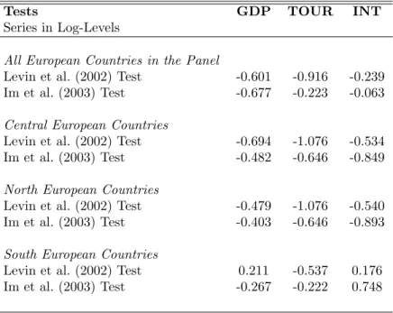
(Insert table 1 here)
Table 16 reports the test results based on the inclusion of an intercept and trend. In every case the null that every variable contains a unit root for the series in logs is not rejected7.
The panel unit root tests applied previously do not account for cross-sectional dependence of the contemporaneous error terms. It has been shown in the literature that failing to consider cross-sectional dependence may cause substantial size distortions, see, for example, Banerjee (1999) and Pesaran (2007). To avoid this mis-performance of the unit root tests we proceed our panel unit root analysis relaxing the assumption of cross sectional independence, employing the test proposed by Moon and Perron (2004) and the test proposed by Pesaran (2007). The Cross-sectionally Augmented IPS Panel Unit Root Test (CIPS) proposed by Pesaran (2007) is a panel fixed effects test allowing for parameter heterogeneity and serial correlation between the cross-sections, correcting their dependency. Within the same line of thought, Moon and Perron (2004) considered a linear dynamic factor model in which the panel is generated by both idiosyncratic shocks and unobserved dynamic factors that are common to all the units, thus explicitly permitting correlation among the cross-sectional units. To avoid specification errors both tests are employed in regressions with an intercept and a trend.
(Insert table 2 here)
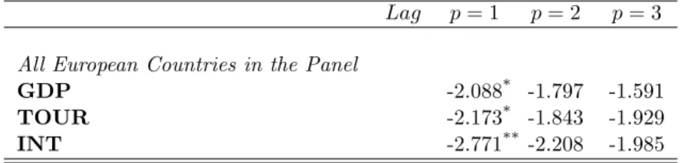
In Table 28 we report the results for the Pesaran cross-sectionally augmented IPS test. The model used to test the unit root hypothesis is the one with intercept and trend. Because our data is annual we test until 3 lag lengths. The unit root test hypothesis is not rejected at the conventional level of significance for the three variables considering a lag length of 2 or 3. These results indicate that variables under investigation are integrated of order 1. Note that, although not shown here, similar results were obtained when we divided the samples according to geographical regions.
(Insert table 3 here)
Moon and Perron panel unit root test results are given in Table 39. Except for the trade variable, all results confirm that for the European countries panel the variables are non stationary at the five percent level. To sum up, it is clear that GDP, real earnings per tourist and total trade volume are I(1) series. Having ascertained the non stationary time series properties of the data, allows us to test for the existence of a cointegration relationship among the variables.
6This estimation was performed using the Rats code that is available upon request to Peter Pedroni.
7To test for the possibility that the variables which were found to be non-stationary are integrated of second
order,I(2), unit root tests on the first differences of the variables were run. Although not shown here, these tests suggest that all variables are stationary in first differences.
8CISP-estimation was performed using the GAUSS code available on line at http:
www.econ.cam.ac.uk/faculty/pesaran/
3
Cointegration Analysis
In this section we report our cointegration analysis results based on three different tests: Pe-droni (1999, 2001, 2004), Larsson and Lyhagen (1999) and Larsson, Lyhagen and Lothgren (2001) likelihood tests. Pedroni panel cointegration test is employed over the entire group of European countries and also considering the smaller geographic groups of North, Central and South Europe. Larsson and Lyhagen tests for cointegration rank are employed over the three geographic groups of European countries. Finally, Larsson et al. (2001) panel cointegration test is employed over the entire group of European countries.
The panel cointegration test proposed by Pedroni (2004) is reported in Table 410. This
residual-based test for the null of no cointegration in heterogeneous panels rejects the null for large negative values. Clearly, from Table 4, the panel statistics indicate fairly support for the hypothesis that real GDP are cointegrated with tourism earnings per tourist arrival and total international trade for the entire group, and also for the sub-sample of Central and South European countries considered in our cointegration analysis.
(Insert table 4 here)
We then implemented the Larsson and Lyhagen (1999) test for Cointegrating Rank for each regional group of European countries. This test has better small sample properties, therefore, it was chosen to analyse each sub-regional group. The Larsson and Lyhagen (1999) Cointegrating Rank tests are given in Table 511 where the Bartlett corrected critical values are obtained by
using the estimated model as data generating process when calculating the sample mean. Us-ing the Bartlett corrected critical values12, the test rejects the null of 0 cointegrating rank but does not reject the null of 1 cointegrating vector at a 5% significance level. Hence, the panel cointegration tests reveal that the common cointegrating rank is one and that the determinis-tic component contains an unrestricted constant and restricted trend. We also employed the likelihood-based cointegration test proposed by Larsson et al. (2001). This test has better large sample properties, so it was used for the whole sample, the 31 European countries’ estimates. These authors propose a likelihood-based test of the cointegrating rank in heterogeneous panels to allow for the possibility of multiple cointegrating vectors. Under the null hypothesis, each group in the panel has at most r cointegrating relationships. Once we calculated the average of the individual Johansen trace statistics (namely the LR-bar statistic), we derived a standard-ized LR-bar statistic to use as the panel cointegration rank test. The setup for the panel vector autoregressive model was modeled as following: we considered as deterministic components an unrestricted intercept and a deterministic trend in the cointegration relationships.
(Insert table 5 here)
The LR-statistic is reported in Table 613 for the entire sample of countries in our panel.
Our results suggest that there is a common cointegration rank in the panel. Compared with the Pedroni tests, Larsson and Lyhagen (1999) and Larsson et al. (2001) tests provide stronger evidence of cointegration among the variables.
(Insert table 6 here)
10This estimation was performed using the Rats code that available upon request to the author. 11This estimation was performed using the GAUSS code available upon request to the authors.
12Given the good size properties of the Bartlett Critical Values (BVC) [see Larsson and Lyhagen (1999)], we
focus our analysis on the BVC test.
4
Estimation of the Long-Run Equilibrium
Our final step is the estimation of the long-run relationships between GDP, tourism earnings per tourist and the total trade volume. In this Section, we begin estimating the long-run equilibrium using the fully-modified OLS (FMOLS) estimator proposed by Pedroni (2000), then we performe the general diagnostic tests for cross section dependence in panels suggested by Pesaran (2004). The hypothesis that there are not cross-sectional dependence is rejected for all regions except for the South European countries. Therefore, we proceed to estimate our panel data model subject to error cross section dependence as suggested by Pesaran (2006).
We estimate the cointegration panel coefficients using the panel fully-modified OLS (FMOLS) estimator proposed by Pedroni (2000).
(Insert table 7 here)
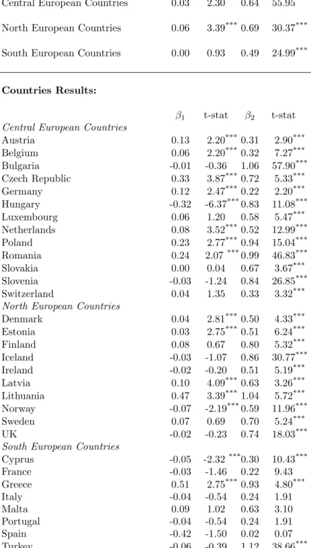
In Table 714 we report Pedroni FMOLS results for cointegration between real GDP, real tourism earnings per tourist arrivals and real total trade volume. β1 is the estimator for tourism
earnings-real GDP elasticity and β2 is the estimator for total trade volume-real GDP elasticity. In regard to the three European regions, most of the coefficients’ estimates are statistically significant, the exception being the slope for the tourism’s coefficient for the South European countries group. Analyzing each coefficient, with reference to all European countries, it is clear from the panel estimates that tourism earnings per tourist arrival play a significant role, such that a 1% increase in this variable leads to a 5% of increase in real GDP. This result is consistent with the results presented in the estimations for individual countries, finding positive effects of tourism development on economic growth. This effect is also found for two of the regional groups studied, namely, Central European countries (with a 3% elasticity) and North European countries (with a 6% elasticity), but is not found for the South European countries (with a 0% not significant elasticity). Simultaneously, we found a positive and significant effect from trade to real GDP for the entire panel and for each regional group. South European countries present a smaller trade elasticity (0.49) than the 0.62% found for the group of all European countries. When analyzing each individual country we note that the most consistent region corresponds to the Central European countries group.15, the estimators concerning tourism activities and total
trade volume seem to be consistent with results obtained for the panel. Some South European countries show individually a negative, even though not significant relationship between tourism and economic growth and, further more, total trade volume is not that relevant for GDP (this may be due to their dependency on imports).
(Insert table 8 here)
In the above analysis, we have to take into consideration that the previous estimation of the cointegration relation does not account for cross-sectional dependence of the contemporane-ous error terms and it has been shown in the literature that failing to consider cross-sectional dependence may cause substantial size distortions, see, for example, O’Connell (1998) and Pe-saran (2007). We performed the general diagnostic tests for cross section dependence in panels suggested by Pesaran (2004) as shown in Tables 8-1116. The hypothesis that there are not cross-sectional dependence is rejected for all regions except for the South European countries.
14This estimation was performed using the Rats code available upon request to the authors.
15Despite the presence of some outliers, such as Czech Republic, Hungary or even Bulgaria, Slovakia and
Slovenia. Observing the data we noticed that prior to 1989, these countries’ data suffered from ’missing data problems’.
Therefore, we proceed to estimate our panel data model subject to error cross section depen-dence as suggested by Pesaran (2006). The Pesaran (2006)’s Monte Carlo simulations show that common correlated effects-Pesaran (2006) pooled estimator (CCE-PPE) has satisfactory small sample17 properties.
(Insert table 9 here)
(Insert table 10 here)
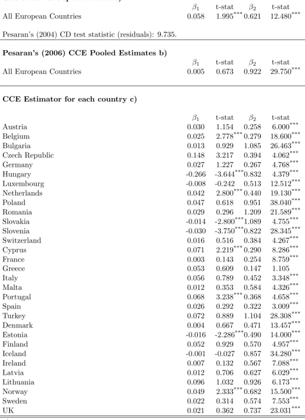
In Table 8 we present the estimation results for the pooled specification for the complete sample as well as for each individual country. Removing the cross dependency, the estimator for the tourism earnings by tourist arrival-GDP elasticity is around 0.5% although not significant. Total trade volume-GDP elasticity moves in opposite direction, augmenting its value towards 92.2% for the set of all European countries. Maybe this result is due to the variable we are using to measure external competitiveness: total trade volume. This variable also measures tourism flows because it contains the item travel and tourism from the current account. Then we are correlating GDP with tourism flows (inbound and outbound) whereas we are correlating GDP with total trade volume. Regarding individual countries estimators, we find a similar performance. The majority has no statistic significance and the values of the tourism earnings by tourist arrival-real GDP elasticities decreases as compared to the estimators obtained by the FMOLS methodology. Once more, total trade volume is the statistically significant variable and showing generalized high magnitude estimators for its elasticities.
(Insert table 11 here)
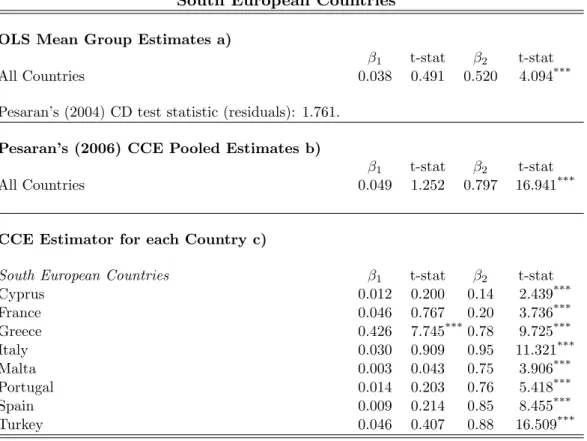
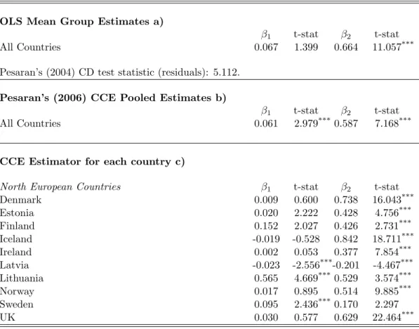
The same estimation technique: common correlated effects-Pesaran (2006) pooled estimator (CCE-PPE) applied to the three regional groups (see Tables 9, 10 and 11) provide similar results to the ones described to the all panel . We find larger coefficients for tourism-GDP elasticity for Central European countries and North European countries when compared to South European countries.
5
Conclusion
This paper applies likelihood-based panel cointegration techniques to examine the existence of a long-run relationship between GDP, tourism earnings per tourist and total trade volume.
Regarding previous work on the effects of tourism on economic growth, we extend the analysis to different regional group of countries, we choose a different proxy for international competi-tiveness and for measuring tourism activity. The countries in the panel are European countries pooled by three geographic regions, Central European countries, South European countries and North European countries. We use total value of trade as a measure of international competi-tiveness in order to be able to differentiate the EURO countries. Since we could not use the real exchange rate, we choose variables that are considered while estimating the long-run value of the real exchange rate. Tourism earnings per tourist is used to proxy tourism activity but since it is in per capita terms it reflects the quality of tourism services provided by each country.
Our results show that there is solid evidence of a panel cointegration relation between tourism and GDP in the European countries. We then performed estimations of the long-run relationship between the variables using the FMOLS estimator. As for the FMOLS estimates, the parame-ters had to be analyzed carefully because we found the presence of common correlated effects.
17Pesaran (2006)’s Monte Carlo simulations also showed that the mean group estimators (CCE-PMG) have
References
Balaguer, J. and Cantavella-Jord´a, M. (2002), ‘Tourism as a long-run economic growth factor: the Spanish case’, Applied Economics34, 877–884.
Banerjee, A. (1999), ‘Panel data unit roots and co-integration: an overview.’, Oxford Bulletin of Economics and Statistics61(0), 607–629.
Bhagwati, J. and Srinivasan, T. (1979),Trade policy and development in international economic policy: theory and evidence, Johns Hopkins University Press, Baltimore, pp. 1–35.
Cort´es-Jimen´ez, I. and Pulina, I. M. (2010), ‘Inbound tourism and long-run economic growth’,
Current Issues in Tourism13, 61–74.
Eugenio-Martin, J. (2004), Tourism and economic growth in latin-american countries: A panel data approach, Nota di Lavoro 26, Fondazione Eni Enrico Mattei Working Paper Series.
Gunduz, L. and Hatemi-J., A. (2005), ‘Is the tourism-led growth hypothesis valid for Turkey?’,
Applied Economics Letters12, 499–504.
Helpman, E. and Krugman, P. R. (1985), Market Structure and Foreign Trade, The MIT Press, Cambridge, Massachussets.
Im, K. S., Pesaran, M. H. and Shin, Y. (2003), ‘Testing for unit roots in heterogeneous panels’,
Journal of Econometrics115, 53–74.
Inkle, L. and Montiel, J. (1999), Exchange Rate Misalignment: Concepts and Measurement for Developing Countries, fifth edn, Oxford University Press, Oxford.
Johansen, S. (1995), Likelihood-based Inference in Co-integrated Vector Autoregressive Models, Oxford University Press, Oxford, UK.
Katircioglu, S. T. (2009), ‘Tourism, trade, and growth: the case of Cyprus’, Applied Economics
41, 2741–2750.
Krueger, A. (1980), ‘Trade police as an input to development’, American Economic Review
70, 188–292.
Larsson, R. and Lyhagen, J. (1999), Likelihood-based inference in multivariate panel cointegra-tion models, Working Paper 331, Stockholm School of Economics, Working paper series in Economics and Finance.
Larsson, R., Lyhagen, J. and Lothgren, M. (2001), ‘Likelihood-based cointegration tests in heterogeneous panels’,Econometrics Journal 4(1), 109–42.
Lee, C. and Chang, C. (2008), ‘Tourism development and economic growth: A closer look at panels’,Tourism Management29, 180–192.
Levin, A., Lin, C.-F. and Chu, C.-S. J. (2002), ‘Unit root tests in panel data: asymptotic and finite-sample properties’,Journal of Econometrics108(1), 1–24.
McKinnon, R. (1964), ‘Foreign exchange constrain in economic development and efficient aid allocation’,Economic Journal74, 388–409.
Nowak, J. J. and Cort´es-Jimen´ez, I. (2007), ‘Tourism, capital goods import and economic growth: theory and evidence for spain’,Tourism Economics13, 515–36.
O’Connell, P. G. (1998), ‘The overvaluation of purchasing power parity’,Journal of International Economics44(1), 1–19.
Oh, C. O. (2005), ‘The contribution of tourism development to economic growth in the Korean economy’,Tourism Management26, 39–44.
Palmer, T. and Riera, A. (2003), ‘Tourism and environmental taxes: with special reference to the balearic ecotax’,Tourism Management24, 665–74.
Pedroni, P. (1999), ‘Critical values for cointegration tests in heterogeneous panels with multiple regressors’,Oxford Bulletin of Economics and Statistics 61, 653–670.
Pedroni, P. (2000), Fully modified OLS for heterogeneous cointegrated panels in Advances in Econometrics: Vol. 15. Nonstationary Panels, Panel Cointegration, and Dynamic Panels., JAI Press, Amsterdam, Holand, pp. 93–130.
Pedroni, P. (2001), ‘Purchasing power parity tests in cointegrated panels’, Review of Economics and Statistics83(4), 727–731.
Pedroni, P. (2004), ‘Panel cointegration; asymptotic and finite sample properties of pooled time series tests, with an application to the ppp hypothesis’,Econometric Theory 20(3), 597–625.
Pesaran, M. (2004), General diagnostic tests for cross section dependence in panels, Working Paper 1233, CESifo.
Pesaran, M. H. (2006), ‘Estimation and inference in large heterogeneous panel with a multifactor error structure’,Econometrica 74(4), 967–1012.
Pesaran, M. H. (2007), ‘A simple panel unit root test in the presence of cross section dependence’,
Appendix
A
DATA
Data used in this article are annual figures covering the period 1988-2010 and variables of this study are real GDP, tourism expenditures by tourist arrival, and real trade volume (total exports plus total imports). Data for GDP and total trade volume are taken from AMECO Database (Eurostat) and for tourism earnings and tourist arrivals from World Travel and Tourism Council (WTTC). Variables, except tourist arrivals, were converted to 2000 US$ constant prices using real exchange rates also taken from AMECO Database.
Data Sources
From the AMECO DatabaseEurostat, it was obtained:
GDP: GDP at current prices for the period 1988-2010.
I N T: Total Trade Volume is total exports plus total imports for the period 1988-2010.
TheWorld Travel and Tourism Council (WTTC)is the source of the following series:
Tables
Table 1: Panel Unit Root Tests
Tests GDP TOUR INT
Series in Log-Levels
All European Countries in the Panel
Levin et al. (2002) Test -0.601 -0.916 -0.239 Im et al. (2003) Test -0.677 -0.223 -0.063
Central European Countries
Levin et al. (2002) Test -0.694 -1.076 -0.534 Im et al. (2003) Test -0.482 -0.646 -0.849
North European Countries
Levin et al. (2002) Test -0.479 -1.076 -0.540 Im et al. (2003) Test -0.403 -0.646 -0.893
South European Countries
Levin et al. (2002) Test 0.211 -0.537 0.176 Im et al. (2003) Test -0.267 -0.222 0.748
The null hypothesis is that the series is a unit root process. An intercept and trend are included in the test equation. The lag length was selected by using the Akaike Information Criteria. The critical values are taken from from Im et al. (2003).
Table 2: Pesaran (2007) Cross-sectionally Augmented IPS (CIPS) Test
Lag p= 1 p= 2 p= 3
All European Countries in the Panel
GDP -2.088* -1.797 -1.591
TOUR -2.173* -1.843 -1.929
INT -2.771** -2.208 -1.985
The null hypothesis is that the series is a unit root process. Critical values for the CIPS test are -3.35 (10%), -2.41 (5%), and -1.89 (1%), see Pesaran (2007).
*Rejects the null at the 10% level. **Rejects the null at the 5% level. ***Rejects the null at the 1% level.
Table 3: Moon and Perron (2004) Panel Unit Root Test
t∗
a t∗b
All European Countries in the Panel
GDP -0.020 -0.416
TOUR -0.012 -0.062
INT 0.076 1.631*
The tests statistics are distributed asN(0,1) under the null of non stationarity. Critical values are 1.28 (10%), 1.64 (5%) and 2.33 (1%).
Table 4: Pedroni (2004) Panel Cointegration Tests
Test Statistic
All European Countries in the Panel -1.277*
Central European Countries -1.829*
North European Countries -0.241
South European Countries -1.980*
The tests statistics are distributed asN(0,1) under the null of no cointegration. The statistics are constructed using small sample adjustment factors from Pedroni (1999, 2004).
Table 5: Larsson and Lyhagen (1999) Tests for Cointegrating Rank
H0 ACVa) BCVb) −2logQT
Central European Countries
R= 0 176.407 265.105 311.999
R≤1 96.513 184.345 162.395
R≤2 39.969 105.135 77.977
North European Countries
R= 0 176.407 265.105 286.727
R≤1 96.513 184.165 149.387
R≤2 39.969 97.852 75.812
South European Countries
R= 0 176.407 265.105 352.628
R≤1 96.513 184.476 165.992
R≤2 39.969 99.669 77.945
a)The asymptotic critical values at 5% significance level. b)Bartlett corrected critical values at 5% significance level.
Table 6: Larsson et al. (2001) Panel Cointegration Test
Standardized LR-bara) R= 0 R≤1
All European Countries in the Panel γLR(H(r)|H(3)) =
√
N√(LR−E(ZK))
V AR(ZK) 8.627 1.382
The null hypothesis is that there are no more than r cointegrating relationships. Critical values are 1.29 at 10% significance level, 1.64 at the 5% level and 2.32 at the 1% level.
a)The moments E(Z
K) and V AR(ZK) are obtained from the procedure described in
Jo-hansen (1995) for the model with a constant and deterministic trend. We used the gauss code sent by the authors upon request. The values obtained for r = 0 were E(ZK) =
Table 7: Panel Estimates of the Cointegration Relationship: FMOLS
Panel Group FMOLS Results:
β1 t-stat β2 t-stat
All European Countries 0.05 3.92***0.62 65.99***
Central European Countries 0.03 2.30***0.64 55.95***
North European Countries 0.06 3.39***0.69 30.37***
South European Countries 0.00 0.93 0.49 24.99***
Countries Results:
β1 t-stat β2 t-stat
Central European Countries
Austria 0.13 2.20***0.31 2.90***
Belgium 0.06 2.20***0.32 7.27***
Bulgaria -0.01 -0.36 1.06 57.90***
Czech Republic 0.33 3.87***0.72 5.33***
Germany 0.12 2.47***0.22 2.20***
Hungary -0.32 -6.37***0.83 11.08***
Luxembourg 0.06 1.20 0.58 5.47***
Netherlands 0.08 3.52***0.52 12.99***
Poland 0.23 2.77***0.94 15.04***
Romania 0.24 2.07***0.99 46.83***
Slovakia 0.00 0.04 0.67 3.67***
Slovenia -0.03 -1.24 0.84 26.85***
Switzerland 0.04 1.35 0.33 3.32***
North European Countries
Denmark 0.04 2.81***0.50 4.33***
Estonia 0.03 2.75***0.51 6.24***
Finland 0.08 0.67 0.80 5.32***
Iceland -0.03 -1.07 0.86 30.77***
Ireland -0.02 -0.20 0.51 5.19***
Latvia 0.10 4.09***0.63 3.26***
Lithuania 0.47 3.39***1.04 5.72***
Norway -0.07 -2.19***0.59 11.96***
Sweden 0.07 0.69 0.70 5.24***
UK -0.02 -0.23 0.74 18.03***
South European Countries
Cyprus -0.05 -2.32***0.30 10.43***
France -0.03 -1.46 0.22 9.43
Greece 0.51 2.75***0.93 4.80***
Italy -0.04 -0.54 0.24 1.91
Malta 0.09 1.02 0.63 3.10
Portugal -0.04 -0.54 0.24 1.91
Spain -0.42 -1.50 0.02 0.07
Turkey -0.06 -0.39 1.12 38.66***
The tests statistics are distributed asN(0,1) under the null of no-cointegration. The test statistics are constructed using small sample adjustment factors from Pedroni (2000, 2004).
Table 8: Panel Estimates of the Cointegration Relationship: CCE-PPE
OLS Mean Group Estimates a)
β1 t-stat β2 t-stat
All European Countries 0.058 1.995***0.621 12.480***
Pesaran’s (2004) CD test statistic (residuals): 9.735.
Pesaran’s (2006) CCE Pooled Estimates b)
β1 t-stat β2 t-stat
All European Countries 0.005 0.673 0.922 29.750***
CCE Estimator for each country c)
β1 t-stat β2 t-stat
Austria 0.030 1.154 0.258 6.000***
Belgium 0.025 2.778***0.279 18.600***
Bulgaria 0.013 0.929 1.085 26.463***
Czech Republic 0.148 3.217 0.394 4.062***
Germany 0.027 1.227 0.267 4.768***
Hungary -0.266 -3.644***0.832 4.379***
Luxembourg -0.008 -0.242 0.513 12.512***
Netherlands 0.042 2.800***0.440 19.130***
Poland 0.047 0.618 0.951 38.040***
Romania 0.029 0.296 1.209 21.589***
Slovakia -0.014 -2.800***1.089 4.755***
Slovenia -0.030 -3.750***0.822 28.345***
Switzerland 0.016 0.516 0.384 4.267***
Cyprus 0.071 2.219***0.290 8.286***
France 0.003 0.143 0.254 8.759***
Greece 0.053 0.609 0.147 1.105
Italy 0.056 0.789 0.452 3.348***
Malta 0.012 0.353 0.584 4.326***
Portugal 0.068 3.238***0.368 4.658***
Spain 0.026 0.292 0.322 3.009***
Turkey 0.072 0.889 1.104 28.308***
Denmark 0.004 0.667 0.471 13.457***
Estonia -0.016 -2.286***0.490 14.000***
Finland 0.052 0.929 0.570 4.957***
Iceland -0.001 -0.027 0.857 34.280***
Ireland 0.007 0.132 0.567 7.088***
Latvia 0.012 0.706 0.627 6.029***
Lithuania 0.096 1.032 0.926 6.173***
Norway 0.049 2.333***0.682 15.500***
Sweden 0.022 0.314 0.574 7.553***
UK 0.021 0.362 0.737 23.031***
a)OLS Mean Group Estimator is simple cross section average of OLS estimator for each cross section unit. b)CCE Pooled Estimator is defined by eq(65) and t-stat is the associated t-ratio of the standard error based
on Newey-West type variance estimator of eq(74) in Pesaran (2006).
c)CCE Estimator for a Country is defined by eq(26) and the corresponding t-stat associated to the standard
error based on Newey-West type variance estimator of eq(50) in Pesaran (2006).
Table 9: Panel Estimates of the Cointegration Relationship: CCE-PPE
Central European Countries
OLS Mean Group Estimates a)
β1 t-stat β2 t-stat
All Countries 0.065 1.585 0.649 8.269***
Pesaran’s (2004) CD test statistic (residuals): 12.617.
Pesaran’s (2006) CCE Pooled Estimates b)
β1 t-stat β2 t-stat
All Countries 0.006 1.120 0.974 50.576***
CCE Estimator for each country c)
Central European Countries β1 t-stat β2 t-stat
Austria 0.023 1.211 0.430 3.071***
Belgium 0.002 0.167 0.550 8.333***
Bulgaria 0.011 1.222 0.959 31.967***
Czech Republic 0.042 0.700 0.473 4.637***
Germany 0.041 1.281 0.306 1.117
Hungary -0.205 -8.542***1.113 23.188***
Luxembourg -0.020 -0.952 0.862 14.131***
Netherlands 0.010 0.714 0.701 18.946***
Poland 0.060 1.538 0.995 71.071***
Romania 0.073 1.217 1.130 35.313***
Slovakia -0.010 -2.500***0.900 4.390***
Slovenia -0.012 -3.000***0.899 64.214***
Switzerland 0.002 0.077 0.922 8.951***
a)OLS Mean Group Estimator is simple cross section average of OLS estimator for each cross section unit. b)CCE Pooled Estimator is defined by eq(65) and t-stat is the associated t-ratio of the standard error based
on Newey-West type variance estimator of eq(74) in Pesaran (2006).
c)CCE Estimator for a Country is defined by eq(26) and the corresponding t-stat associated to the standard
error based on Newey-West type variance estimator of eq(50) in Pesaran (2006).
Table 10: Panel Estimates of the Cointegration Relationship: CCE-PPE
South European Countries
OLS Mean Group Estimates a)
β1 t-stat β2 t-stat
All Countries 0.038 0.491 0.520 4.094***
Pesaran’s (2004) CD test statistic (residuals): 1.761.
Pesaran’s (2006) CCE Pooled Estimates b)
β1 t-stat β2 t-stat
All Countries 0.049 1.252 0.797 16.941***
CCE Estimator for each Country c)
South European Countries β1 t-stat β2 t-stat
Cyprus 0.012 0.200 0.14 2.439***
France 0.046 0.767 0.20 3.736***
Greece 0.426 7.745***0.78 9.725***
Italy 0.030 0.909 0.95 11.321***
Malta 0.003 0.043 0.75 3.906***
Portugal 0.014 0.203 0.76 5.418***
Spain 0.009 0.214 0.85 8.455***
Turkey 0.046 0.407 0.88 16.509***
a)OLS Mean Group Estimator is simple cross section average of OLS estimator for each cross section unit. b)CCE Pooled Estimator is defined by eq(65) and t-stat is the associated t-ratio of the standard error
based on Newey-West type variance estimator of eq(74) in Pesaran (2006).
c)CCE Estimator for a Country is defined by eq(26) and the corresponding t-stat associated to the
standard error based on Newey-West type variance estimator of eq(50) in Pesaran (2006).
Table 11: Panel Estimates of the Cointegration Relationship: CCE-PPE
North European Countries
OLS Mean Group Estimates a)
β1 t-stat β2 t-stat
All Countries 0.067 1.399 0.664 11.057***
Pesaran’s (2004) CD test statistic (residuals): 5.112.
Pesaran’s (2006) CCE Pooled Estimates b)
β1 t-stat β2 t-stat
All Countries 0.061 2.979***0.587 7.168***
CCE Estimator for each country c)
North European Countries β1 t-stat β2 t-stat
Denmark 0.009 0.600 0.738 16.043***
Estonia 0.020 2.222 0.428 4.756***
Finland 0.152 2.027 0.426 2.731***
Iceland -0.019 -0.528 0.842 18.711***
Ireland 0.002 0.053 0.377 7.854***
Latvia -0.023 -2.556***-0.201 -4.467***
Lithuania 0.565 4.669***0.529 3.574***
Norway 0.017 0.895 0.514 9.885***
Sweden 0.095 2.436***0.170 2.297
UK 0.030 0.577 0.629 22.464***
a)OLS Mean Group Estimator is simple cross section average of OLS estimator for each cross section unit. b)CCE Pooled Estimator is defined by eq(65) and t-stat is the associated t-ratio of the standard error based
on Newey-West type variance estimator of eq(74) in Pesaran (2006).
c)CCE Estimator for a Country is defined by eq(26) and the corresponding t-stat associated to the standard
error based on Newey-West type variance estimator of eq(50) in Pesaran (2006).