An ILS-based algorithm to solve a large-scale real heterogeneous ﬂeet VRP with multi-trips and docking constraints

(1)

Contents lists available atScienceDirect

European Journal of Operational Research

journal homepage:www.elsevier.com/locate/ejor

Discrete Optimization

An ILS-based algorithm to solve a large-scale real heterogeneous ﬂeet

VRP with multi-trips and docking constraints

V. N. Coelho

a,∗

_{, A. Grasas}

b

_{, H. Ramalhinho}

c

_{, I. M. Coelho}

d,f

_{, M. J. F. Souza}

e

_{, R. C. Cruz}

a a_{Department of Control and Automation Engineering, Federal University of Ouro Preto, Ouro Preto, MG, 35400-000, Brazil}

b_{Department of Marketing, Operations and Supply, EADA Business School, Barcelona, 08011, Spain} c_{Department of Economics and Business, Universitat Pompeu Fabra, Barcelona, 08005, Spain} d_{Institute of Computing, Fluminense Federal University, Niterói, 24210-240, Brazil}

e_{Department of Computer Science, Federal University of Ouro Preto, Ouro Preto, MG, 35400-000, Brazil} f_{Department of Computer Science, State University of Rio de Janeiro, Rio de Janeiro, Brazil}

a r t i c l e

i n f o

Article history:

Received 25 September 2014 Accepted 16 September 2015 Available online 1 October 2015

Keywords: VRP

Heterogeneous ﬂeet Multiple trips Docking constraints Iterated local search

a b s t r a c t

Distribution planning is crucial for most companies since goods are rarely produced and consumed at the same place. Distribution costs, in addition, can be an important component of the final cost of the products. In this paper, we study a VRP variant inspired on a real case of a large distribution company. In particular, we consider a VRP with a heterogeneous fleet of vehicles that are allowed to perform multiple trips. The problem also includes docking constraints in which some vehicles are unable to serve some particular customers, and a realistic objective function with vehicles’ fixed and distance-based costs and a cost per customer visited. We design a trajectory search heuristic called

GILS-VND

that combines Iterated Local Search (

ILS

), Greedy Randomized Adaptive Search Procedure (

GRASP

) and Variable Neighborhood Descent (

VND

) procedures. This method obtains competitive solutions and improves the company solutions leading to signiﬁcant savings in transportation costs.

1. Introduction

Vehicle routing problems (VRP) seek to find routes to deliver goods from a central depot to a set of geographically dispersed cus-tomers. These problems, faced by many companies, are crucial in dis-tribution and logistics due to the need of finding cost-effective routes providing high customer satisfaction. The classical routing problem, first proposed byDantzig and Ramser (1959)and known as Capaci-tated VRP, has the objective of minimizing the total distance traveled by a homogeneous fleet of vehicles to serve the demands of all cus-tomers. Although this problem has been studied for more than five decades (Laporte, 2009), real applications remain a challenge. They feature a variety of operational restrictions and rules that complicate the problem and may have a significant impact on the solution. These additional considerations may affect customers, depots, and vehicles, for example.

∗ _{Corresponding author. Tel.: +55 3135514407 .}

E-mail addresses: vncoelho@gmail.com (V.N. Coelho), agrasas@eada.edu (A. Grasas), helena.ramalhinho@upf.edu (H. Ramalhinho), imcoelho@ic.uff.br (I.M. Coelho),marcone@iceb.ufop.br(M.J.F. Souza),phaelcarlos@gmail.com(R.C. Cruz).

In this paper, we study a real VRP variant of a major distribution company in Europe that serves around 400 customers. This version of the problem addresses the following considerations:

1. Limited heterogeneous ﬂeet of vehicles: the company owns a ﬂeet composed of different vehicle types;

2. Possibility of vehicles performing multiple trips;

3. Docking constraints that restrict certain customers to be served by certain types of vehicles;

4. For each vehicle, a ﬁxed and variable (transportation) cost.

This problem is a variant of the Heterogeneous Fleet Multi-trip Vehicle Routing Problem (HFMVRP) introduced byPrins (2002). This new variant includes docking constraints and a different objective function. The goal is to minimize the total cost composed of (i) a ﬁxed cost for using each vehicle, (ii) a ﬁxed cost per customer visited, and (iii) a variable vehicle-dependent cost per distance traveled. Besides minimizing total distribution costs, for managerial reasons the com-pany is also concerned about three other routing indicators, namely, (i) the total number of routes employed, (ii) the total distance trav-eled, and (iii) the vehicles’ idle capacity. Their purpose, apart from saving costs, is to have the least number of routes with full truckload vehicles.

http://dx.doi.org/10.1016/j.ejor.2015.09.047

(2)

The HFMVRP is anN P-Hard problem, and, as such, exact methods have restricted applicability to obtain good solutions. Heuristic meth-ods, like the one presented in this paper, are the most common ap-proach to solve this type of problems. In particular, we use a heuristic algorithm, the

GILS-VND, that combines three different procedures:

1. Iterated Local Search (ILS) (Lourenço, Martin, & Stützle, 2003; Stützle, 2006);

2. Greedy Randomized Adaptive Search Procedure (GRASP) (Feo & Resende, 1995; Resende & Ribeiro, 2010);

3. Variable Neighborhood Descent (VND) (Mladenovi ´c & Hansen, 1997).

We test our algorithm using real instances provided by the com-pany. The algorithm proved to be fast and reliable, and the solutions obtained were better than those implemented by the company in all instances and dimensions. Overall, the major contributions of the cur-rent work are:

• The study of a routing problem of a real company that includes docking constraints, a heterogeneous ﬂeet and multi-trips, and with a realistic cost function based on distance, type of vehicle and customers visited.

• The design of a trajectory search metaheuristic combining

ILS,

GRASP

and

VND.

• The development of a new multi-trip constructive method in-spired by the Clarke and Wright Savings procedure.

• The application of efficient Auxiliary Data Structures to optimize the search process in the proposed neighborhood structures.

The remainder of this paper is organized as follows.Section 2 re-views the literature on heterogeneous VRPs.Section 3deﬁnes for-mally the HFMVRP with docking constraints.Section 4describes the

GILS-VND

algorithm used to solve this problem.Section 5presents some computational experiments, and ﬁnallySection 6draws the ﬁ-nal considerations.

2. Heterogeneous VRPs

VRPs with heterogeneous fleet (HVRP) can be divided according different features (Penna, Subramanian, & Ochi, 2013), including the vehicle availability (limited or unlimited) and vehicle costs (fixed or variable). When the fleet is limited, the number of vehicles and their capacity are known beforehand, and solution routes must consider this availability. In the case of unlimited fleet, however, the required number of vehicles to meet customer demands is unknown initially, and the problem must determine the fleet composition considering the vehicles’ cost and capacity.

To the best of our knowledge, the first paper in the literature that involves an unlimited fleet with fixed costs was proposed byGolden, Assad, Levy, and Gheysens (1984). This problem is also referred as the Fleet Size and Mix VRP. The authors designed two heuristic methods to solve the problem: one based on best insertion and the other based on the classical Clarke and Wright Savings (CWS) heuristic (Clarke & Wright, 1964). The latter outperformed the former. They also de-veloped a mathematical formulation for the variant with dependent costs, and obtained the first lower bounds for the VRP with unlimited fixed fleet. More studies on HVRPs with unlimited fleet came there-after.Gendreau, Laporte, Musaraganyi, and Taillard (1999)included investment costs in the medium term and short-term operating costs that fluctuated according to the specific customers attended per day. The authors suggested an algorithm based on Tabu Search (TS) with a tour construction phase and an improvement phase that consid-ered variable costs. They, however, assumed Euclidean problems only, where nodes were located in the same plane.Choi and Tcha (2007) obtained lower bounds for all variants of the unlimited fleet prob-lem using a column generation approach based on the set covering problem.Baldacci and Mingozzi (2009)proposed a variant based on

a set partitioning problem that used bounds provided by a procedure based on the Linear and Lagrangian relaxation. The procedure was ap-plied to solve the main variants of the problem involving limited and unlimited ﬂeet, with costs and dependent variables. The proposed method was able to solve instances with up to 100 customers, pre-senting itself as the state-of-the-art exact algorithm applied to the problem.Brandão (2009)followed the basic ideas ofGendreau et al. (1999)using a deterministic

TS

algorithm for the ﬂeet size and mix VRP.

Among the heuristic approaches presented in the literature, note-worthy are those based on Evolutionary Algorithms. Ochi, Vianna, Drummond, and Victor (1998)developed an algorithm that combines a Genetic Algorithm (GA) with Scatter Search.Liu, Huang, and Ma (2009)proposed a hybrid

GA

with a hybrid local search procedure. Prins (2009)presented two Memetic Algorithms. The ﬁrst approach used a chromosome encoded as a giant tour, and a split procedure that performed the optimal distribution of vehicles and routes. The second algorithm used distance calculation strategies in order to di-versify the search in the solution space.Tütüncü (2010)proposed a visual interactive approach based on a greedy randomized adaptive memory programming search algorithm to study an HVRP variant with backhauls.Penna et al. (2013)devised an algorithm based on

ILS

which used a random

VND

in the local search phase. More stud-ies on different variants of the HVRP are compiled byBaldaccci, Bat-tarra, and Vigo (2008),Imran, Salhi, and Wassan (2009)andVidal, Crainic, Gendreau, and Prins (2013).

The HVRP is gaining attention from researchers due to its applica-bility in real cases. In the past years, a variety of papers, including this one, have addressed more realistic setups involving a heterogeneous fleet with additional constraints.Belfiore, Yoshizaki, and Tsugunobu (2009)studied a real-life HVRP with time windows and split deliv-eries in a major Brazilian retail group. The authors generated some initial solutions that were improved by scatter search.Kritikos and Ioannou (2013)addressed an HVRP with time windows, in which some vehicles were loaded above their nominal capacity (overloads). The authors developed a sequential insertion heuristic with a com-ponent in the selection criteria of the non-routed customers and a penalty in the objective function for overloads.Leung, Zhang, Zhang, Hua, and Lim (2013)analyzed a two-dimensional loading HVRP us-ing a simulated annealus-ing with a heuristic local search.Ribeiro, De-saulniers, Desrosiers, Vidal, and Vieira (2014)studied the workover rig routing problem, which can be seen as a variation of the VRP without a depot. In the workover rig routing problem, routes of a heterogeneous fleet of rigs need to be found to minimize the total production loss of the wells over a finite horizon. The authors pro-posed and compared four heuristics: a variable neighborhood search heuristic, a branch-price-and-cut heuristic, an adaptive large neigh-borhood search heuristic and a hybrid

GA. Another application of

the adaptive large neighborhood search method was presented by Amorim, Parragh, Sperandio, and Almada-Lobo (2014). The authors considered a real heterogeneous ﬂeet site dependent VRP with mul-tiple time windows faced by a Portuguese food distribution company. Jiang, Ng, Poh, and Teo (2014)also studied an HVRP with time win-dows and employed a two-phase

TS

algorithm.Dayarian, Crainic, Gendreau, and Rei (2015)designed a branch-and-price methodology to tackle a real-life milk collection problem with heterogeneous ﬂeet, multi-depot and other resource constraints. Another real application was handled byde Armas and Melián-Batista (2015), who proposed a variable neighborhood search algorithm to solve an HVRP with mul-tiple and soft time windows and customers’ priorities. Although the problems exposed in this paragraph and our problem have different constraints, most of the algorithms designed to solve them rely on heuristic searches like

ILS

or variable neighborhood search.

(3)

Caceres-Cruz et al. (2014, Section 3). Our problem and these other two problems are routing problems that include a heterogeneous ﬂeet with the possibility of performing multiple trips (HFMVRP). On one hand,Prins (2002)studied a large-scale real case of a French furni-ture manufacfurni-turer with 775 stores. In Prins’ problem, a time restric-tion of 5 hours on routes was imposed and the largest demand of a store could not exceed the smallest vehicle’s capacity. The author developed a

CWS-based algorithm with two heuristics, New Merge

Heuristic (MER) and

MER2, to address the single- and the multi-trip

problems, respectively. The algorithm solutions were improved via a steepest descent local search and a tabu search with a simple biob-jective approach: minimizing the total duration of all trips and the number of vehicles. The results obtained outperformed the solutions used by the furniture company. On the other hand,Caceres-Cruz et al. (2014)also studied an HVRP with multi-trips inspired on the same distribution company that is discussed in the present work. The au-thors built a randomized hybrid algorithm based on the

CWS

heuris-tic, called

Rand-MER. The

{

(

i,j

)

|

i,j∈

V,i< j

}

represent the vertices and the edges of the graph, respec-tively. The depot is denoted by 0 and verticesi∈Vࢨ{0} represent the ncustomers, each one with a nonnegative demandd_i. Each edge (i,j)

∈Ehas an associated nonnegative cost or distancecij. There is a ﬂeet Tcomposed ofmdifferent types of vehicles, i.e.,T=

{

1, . . . ,m

}

. For eacht∈Tthere aremtavailable vehicles with capacityqt(in boxes of products), ﬁxed costcftper vehicle used, and variable costcdtper distance traveled. There is also a ﬁxed costcctincurred per customer visited.

We letS=

{

(

r,t

)

|

t∈T,r=

(

v

₀_,

v

₁_{, . . . ,}

v

_n₍_r₎

+1

)

}

This set of features characterizes the HFMVRP tackled in this work. The problem seeks to build a setS∗_{that minimizes the total cost}

func-tion given by: TC=

(r,t)∈S Ct

r (1)

Note that the cost of a route,Ct

r,is composed of three cost terms. For convenience, we group these terms by type for all routes and express the objective function asTC=CF+CC+CDwhere:

•C_F=₍_r,t₎_∈_Sc ftis the total ﬁxed cost of the vehicles used. •CC=(r,t)∈Sn

(

r

)

×cctis the total cost of the customers visited. •CD=(r,t)∈Scdtn_i₌(r₀)cv

i,v

i+1is the total cost of the distance

trav-eled by all vehicles.

A valid route must satisfy the following criteria:

1. Each route must start and end at the depot. 2. Each customer is assigned to exactly one route.

3. Each customer must be compatible with the vehicle type assigned to its route, i.e., given a route (r,t),

∀

and 0 otherwise.

4. The sum of customer demands in the route cannot exceed the maximum capacity of the vehicle typetassigned to that route, i.e.,Qt

r≤qt.

5. Each vehicle type can perform one or two routes, that is, it can be a single- or a multi-trip vehicle, respectively.

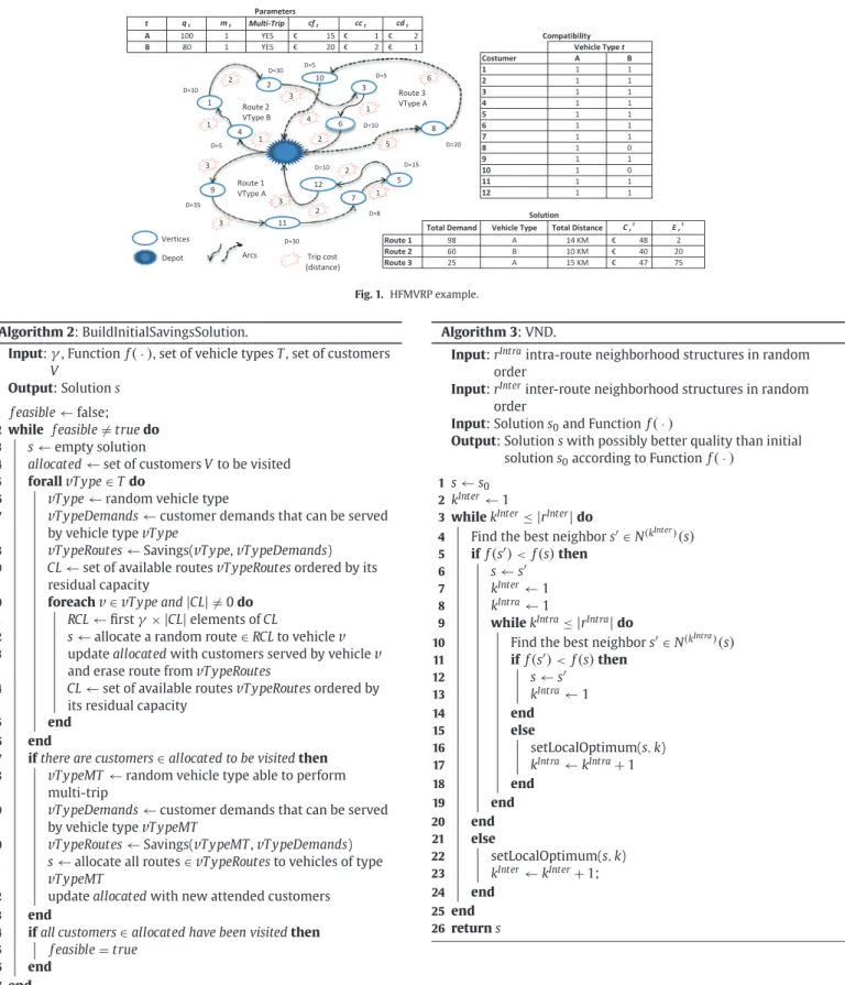
Fig. 1displays a solution example for an HFMVRP with 12 cus-tomers, 2 types of vehicles, and only one vehicle per type. The “Pa-rameters” table shows the parameter values for each vehicle type. The “Compatibility” table indicates the values ofcomp(t,i), fort∈{A, B} andi∈Vࢨ{0}. Note that a type B vehicle cannot visit customers 8 or 10. The “Solution” table displays the resulting routes, with the total demand served, distance traveled, total cost and residual capac-ity. Note that the vehicle type A performs two routes, 1 and 3. The graph shows the sequence of the three routes: vertices have the cor-responding customer demand, and arcs the corcor-responding distance next to them. For this example,CF =50,CC=17,CD=68,and the total cost isTC=135.

4. Methodology

4.1. The GILS-VND algorithm

The algorithm proposed in this paper, dubbed

GILS-VND,

com-bines an Iterated Local Search (ILS), a Greedy Randomized Adap-tive Search Procedure (GRASP), and a Variable Neighborhood De-scent (VND). Its pseudocode is outlined inAlgorithm 1. It requires the following input parameters: (i)GRASPmaxis the number of

GRASP

executions to construct an initial solution, (ii)IterMaxis the maxi-mum number of iterations performed at a given perturbation level, (iii)

γ

restricts the size of the candidate list, and (iv) the objec-tive function f(·) (Eq. (1) deﬁned in Section 3). The

GILS-VND

Algorithm 1: GILS-VND.

Input:GRASPmax,IterMax,

γ

, Functionf

(

·

)

Output: Solutions

s0←best solution inGRASPmaxiterations of the procedure 1

BuildInitialSavingsSolution (

γ

) s∗_←_VND(s

0,f) 2

p←0 3

while stop criterion not satisfieddo

4

iter←0 5

while iter<IterMaxandstop criterion not satisfieddo

6

s′_←_Reﬁne(s∗_,_p_,_f)

7

if f

(

s′

₎

_<_f

₍

_s∗

₎

_then

8

s∗_←_s′_; 9

p←0; 10

iter←0 11

end 12

else 13

iter←iter+1 14

end 15

end 16

p←p+1 17

end 18

returns

(4)

Fig. 1. HFMVRP example.

Algorithm 2: BuildInitialSavingsSolution.

Input:

γ

, Functionf

(

·

)

, set of vehicle typesT, set of customers

V

f easible←false; 1

while f easible=truedo

2

s←empty solution 3

allocated←set of customersVto be visited 4

forall

v

T ype∈Tdo

residual capacity

T ypeMT_←random vehicle type able to perform

18

multi-trip

v

T ypeDemands←customer demands that can be served 19

T ypeRoutesto vehicles of type

21

v

T ypeMT

updateallocatedwith new attended customers 22

end 23

ifall customers∈allocated have been visitedthen 24

f easible=true 25

end 26

end 27

returns

28

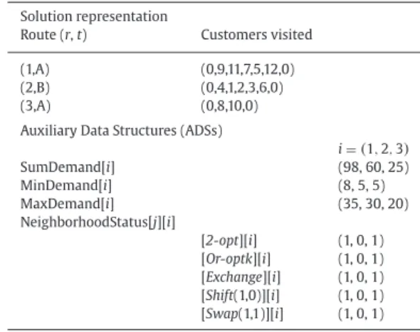
algorithm works as follows. Line 1 calls the BuildInitialSavingsSo-lution procedure to obtain the best initial soBuildInitialSavingsSo-lution afterGRASPmax runs (Algorithm 2). Line 2 calls the

VND

procedure to perform a local search (Algorithm 3). Line 3 initializesp, a variable that regulates the “power” of diversiﬁcation, and lines 4–18 perform the main

ILS

loop

Algorithm 3: VND.

Input:rIntra_{intra-route neighborhood structures in random}

order

Input:rInter_{inter-route neighborhood structures in random}

order

Input: Solutions0and Functionf

(

·

)

Output: Solutionswith possibly better quality than initial

solutions0according to Functionf

(

·

)

s←s0

1

kInter_←₁ 2

whilekInter_≤

_|

_rInter

_|

_do 3

Find the best neighbors′_∈_N(kInter₎

(

s

)

4

iff

(

s′

₎

_< _f

₍

_s

₎

_then 5

s←s′ 6

kInter_←₁ 7

kIntra_←₁ 8

whilekIntra_≤

_|

_rIntra

_|

_do 9

Find the best neighbors′_∈_N(kIntra₎

(

s

)

10

iff

(

s′

₎

_< _f

₍

_s

₎

_then 11

s←s′ 12

kIntra_←₁ 13

end 14

else 15

setLocalOptimum(s,k) 16

kIntra_←_kIntra₊₁ 17

end 18

end 19

end 20

else 21

setLocalOptimum(s,k) 22

kInter_←_kInter₊_1; 23

end 24

end 25

returns

26

while the stopping condition is not satisﬁed. Within the

ILS, line 7

calls the Reﬁne procedure that perturbs the solution (Algorithm 4). Line 19 then returns the ﬁnal solution.

(5)

is, routes with total demand closer to the capacity of the current allocated vehicle type,

v

T ype,are listed ﬁrst. In this sense, routes that have its demand equal to the capacity of the vehicle are the most coveted. The input parameter

γ

regulates the size of the candidate list. All available vehicles of the vehicle type

v

T ypeare assigned to

a route until

v

_{T ypeRoutes}_{is empty or vehicles of that type are}

al-ready allocated (line 10). If there are still customers to be allocated after this ﬁrst phase, a vehicle type able to perform multi-trips is se-lected and all customers with demand lower or equal to that vehicle capacity are allocated and grouped according to the same Clarke and Wright Savings algorithm (lines 17 to 23). Line 22 updates the vec-torallocatedwith the clients attended by multi-trip vehicles of type

v

T ypeMT. If customers remain still unassigned (line 24), the

proce-dure is repeated.

Algorithm 4: Reﬁne.

Input:rpert_{perturbation neighborhoods in random order}

Input: Initial solutions, Levelpand Functionf

(

·

)

fori←1Top+2do

1

k←SelectNeighborhood(rpert₎ 2

s′_←_Shake(s_,_k) 3

end 4

s←VND

(

s′_,_f

₎

5

returns

6

The

VND

procedure (Algorithm 3) performs a local search using the neighborhood structures described inSection 4.2. The exploration is done via inter-route movements (line 4) and intra-route move-ments (line 10). Lines 16 and 22 trigger the setLocalOptimum pro-cedure, which sets neighborhoods as “local-optimum”. This mark is used by the auxiliary data structure NeighborhoodStatus[j][i], de-scribed inSection 4.3.

The Reﬁne procedure (Algorithm 4) takes the current solution,s∗_,

selects randomly the neighborhood structures,rpert_{(line 2), and} per-forms a shake (line 3). This is done iteratively (lines 1–4) according to the variablep. If a given solution is not improved for a number of iterMaxiterations (line 6 ofAlgorithm 1), variablepis incremented (line 17 ofAlgorithm 1) so thatp+2 random moves (shakes) will be applied to the current solution. This mechanism balances exploration against exploitation.

4.2. Neighborhood structures

Five different neighborhood structures are applied to explore the solution space of the problem. The ﬁrst three are intra-route move-ments while the last two are inter-route movemove-ments. It is important to note that movements that lead to infeasible solutions are not al-lowed.

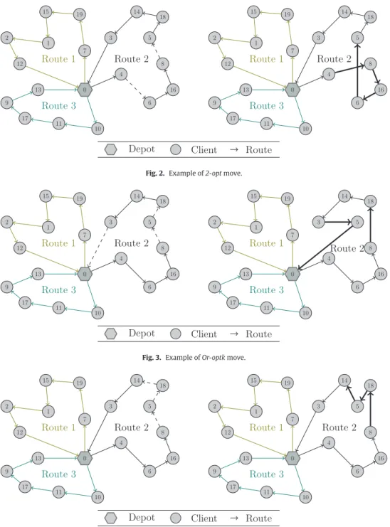
2-opt move: A 2-opt move is an intra-route movement that consists in removing two non-adjacent arcs and inserting two new arcs, so that a new route is formed.Fig. 2exempliﬁes the movement: edges (4, 6) and (8, 5) of Route 2 are removed and edges (4, 8) and (6, 5) are inserted instead. Note that an inversion took place involving customers 6, 16 and 8, and now the sequence is 8–16–6. For a symmetric problem, the total distance among these customers remains unaffected.

Or-optkmove: AnOr-optkmove is an intra-route movement that consists in removing k consecutive customers from a given route and reinserting them into another position of the same route. This move is a generalization of the Or-opt proposed by Or (1976), in which the removal involves up to three consecutive customers only. Fig. 3 illustrates the movement withk=1, where customer 5 is

Table 1 HFMVRP solution.

Solution representation

Route (r,t) Customers visited

(1,A) (0,9,11,7,5,12,0)

(2,B) (0,4,1,2,3,6,0)

(3,A) (0,8,10,0)

Auxiliary Data Structures (ADSs)

i=(1,2,3)

SumDemand[i] (98, 60, 25)

MinDemand[i] (8, 5, 5)

MaxDemand[i] (35, 30, 20)

NeighborhoodStatus[j][i]

[2-opt][i] (1, 0, 1) [Or-optk][i] (1, 0, 1) [Exchange][i] (1, 0, 1) [Shift(1,0)][i] (1, 0, 1) [Swap(1,1)][i] (1, 0, 1)

moved to the last position of Route 2. For this particular case when k=1,the movement is also known as Reinsertion in the literature (Subramanian, Uchoa, & Ochi, 2013).

Exchangemove: AnExchangemove is an intra-route movement that consists in exchanging two customers in the same route.Fig. 4 shows anExchangeof customers 5 and 18 in Route 2.

Shift(1,0) move: AShift(1,0) move is an inter-route movement that relocates a customer from one route to another.

Swap(1,1) move: ASwap(1,1) move is an inter-route movement that exchanges two customers from different routes.

All neighborhood structures are used as a perturbation strategy. The application of these moves occurs randomly with no improve-ment veriﬁcation in the objective function. This mechanism is a key to diversify and explore the solution space (exploration-exploitation). After applying a given move, the NeighborhoodStatus[j][i] vector (de-scribed below) is updated.

4.3. Auxiliary Data Structures (ADSs)

In order to intensify and optimize the search of the neighbor-hood structures, some Auxiliary Data Structures (ADSs) ofPenna et al. (2013)have been adapted and applied to the multi-trip HFMVRP. A brief description is given below:

Fori∈

{

1, . . . ,#nRoutes

}

andj∈

{

1, . . . ,#nNeighborhoods

}

the fol-lowing data structures are used. Variable #nRoutesindicates the total number of routes and #nNeighborhoodsthe number of neighborhood structures (seeSection 4.2).

• SumDemand[i]: it stores the sum of all customer demands as-signed to routei.

• MinDemand[i]: it stores the minimum demand among all cus-tomers in routei.

• MaxDemand[i]: it stores the maximum demand among all cus-tomers in routei.

• NeighborhoodStatus[j][i]: it is a boolean value that indicates whether the neighborhoodjis in a local optimum regarding route i. Upon a full application of all neighboring structures by a lo-cal search method, all routes are marked as “lolo-cal-optimum”. When a solution is “shaked” (Line 3 ofAlgorithm 4), some “local-optimum” markers are removed from the routes that have been affected by that perturbation.

(6)

Fig. 2.Example of2-optmove.

Fig. 3.Example ofOr-optkmove.

Fig. 4. Example ofExchangemove.

5. Computational experiments

The

GILS-VND

algorithm was implemented in C++with assis-tance from OptFrame framework (http://sourceforge.net/projects/ optframe/). This optimization framework has been successfully applied in guiding the implementation of neighborhood structures (see Coelho et al., 2012). In general, frameworks are based on the researchers’ experience with the implementation of multiple methods for different problems (Coelho et al., 2011). For instance, Souza et al. (2010) andCoelho et al. (2014) employed OptFrame to an open-pit-mining problem, and to load energy forecasting, respectively. The computational framework OptFrame has, be-sides standardized optimization structures, statistical and checking modules which are able to provide the ability of verifying the consistency of the new designed method (as will be described in Section 5.1).

(7)

Table 2

CheckModuleOutput – computational times.

Component #Tests Average(milliseconds)

Test 1: building an initial solution

Constructive 30 40,568

Test 2: update cost of the ADS

ADSManager 94,885 0.1222

Test 3: complete evaluation of a solution

Evaluator 94,885 0.0385

Test 4: cost ofapplymethod

2-Opt 256 0.0039

Or-opt1 708 0.0039

Exchange 1144 0.0035

Shift(1,0) 12,986 0.0074

Swap(1,1) 33,402 0.0071

Test 5: calculating the cost of a move

2-Opt 128 0.0783

2-Opt-Optimized 128 0.0014

Or-opt1 354 0.0799

Or-opt1-Optimized 354 0.0014

Exchange 572 0.0790

Exchange-Optimized 572 0.0015

Shift(1,0) 6493 0.0921

Shift(1,0)-Optimized 6493 0.0016

Swap(1,1) 16,701 0.0917

Swap(1,1)-Optimized 16,701 0.0016

Table 3

CheckModuleOutput – efficiency of the neighborhood structures.

Average number of moves from neighborhood in 30 tests

Neighborhood

Valid neighborhood

moves Standard Optimized Imp. (%)

2-Opt 154 869 869 0.00

Or-opt1 426 3,030 3,030 0.00

Exchange 688 3,030 3,030 0.00

Shift(1,0) 7,813 738,630 8,106 98.90

Swap(1,1) 20,097 296,258 69,307 76.60

good balance between cost and residual capacity in the candidate routes.

The next three sections describe the computational experiments conducted to measure the efficiency of the algorithm.Section 5.1 evaluates the neighborhood structure efficiency. Section 5.2 mea-sures the time required to reach the solution currently used by the company, based on run time distributions. Finally,Section 5.3 pro-vides detailed results with all costs involved comparing

GILS-VND,

Rand-MER

and the company solutions.

5.1. Detailed results on algorithm implementation

The ﬁrst experiment aims at verifying the quality and efficiency of the neighborhood structures implemented in the

GILS-VND

algorithm. Tables 2 and 3 exhibit the typical indicators from

checkModule’s output of the OptFrame framework. The ﬁrst

col-umn inTable 2indicates the OptFrame component. All ﬁve neigh-borhood structures are implemented in OptFrame core as sequential neighborhoods. The “Optimized” neighborhood structures have an efficient reimplementation that discards inter-route moves that vi-olate maximum capacities of a given vehicle (vectors SumDemand[i], MinDemand[i] and MaxDemand[i] helped in this task). The number of tests for each component and the average time spent in each ex-periment are displayed in the second and third columns ofTable 2, respectively.

Tests 1 and 2 display the computational time to build an initial so-lution and the ADS, respectively. Thirty initial soso-lutions were gener-ated with an average time of 0.041 seconds per solution, and 94,885 different feasible solutions were considered through the neighbor-hood structures described inSection 4.2. Test 3 indicates the average

time spent to evaluate a solution. Test 4 shows the time required to apply each move generated by the neighborhood structures. Shift(1,0) move is the most costly to apply, requiring 0.0074 milliseconds. This result is consistent since this move changes the size of routes. Test 5 shows the computational time spent to calculate the cost of the move, i.e., the impact on the evaluation function of changing to the selected neighbor. In the “Optimized” version of each neighborhood, the cost calculation beneﬁts from ADSs, not needing to perform the change in the solution and to recalculate the objective function value. This strategy improved the execution time up to 57.6 times for the neighborhood Shift(1,0), reducing the average time from 0.0921 to 0.0016 milliseconds.

On the other hand,Table 3shows the average number of solutions generated by each neighborhood structure in 30 tests. The second col-umn indicates the average number of moves that lead to other feasi-ble solutions; the third and fourth columns indicate the average num-ber of moves generated by the standard OptFrame implementation and the OptFrame implementation using ADSs, respectively, and the last column indicates the percentage reduction of ineffective moves calculated usingEq. (2).

Impro

v

ement

(

%

)

=Standard−Optimized

Standard ∗100 (2) Clearly, the use of standard neighborhood structures provided by OptFrame and the implementation of efficient ADSs led to a drastic reduction in the number of moves to find the same number of valid solutions: 98.90% and 76.60% less moves for Shift(1,0) and Swap(1,1), respectively. This improvement is achieved mainly because most of the infeasible solutions can be disregarded directly before proceed-ing further just by analyzproceed-ing the values of the ADSs. Many moves from the Swap and Shift neighborhood structures lead to infeasible solutions, i.e., the vehicle’s capacity and/or docking constraint are vi-olated because a new customer from another route is included. Al-though the proposed algorithm may still reach the same final so-lution (since infeasible soso-lutions can be discarded after evaluation), OptFrame provides two specific mechanisms to avoid such unneces-sary moves and calculations. The first mechanism is to use the pre-computed information in the ADS to disallow the selection of moves that could violate constraints (e.g., by testing whether the customer to be inserted in the route has a bigger demand than the vehicle’s idle capacity). In that case, the move is never generated by the itera-tor nor applied to the current solution. The second mechanism is to avoid the generation of moves corresponding to a local optimum of specific neighborhood structures. For example, if the first route is in a local optimum regarding all intra-route neighborhood structures, a future intra-route move will never be tested in this route unless a perturbation or an inter-route move has removed that route from the local optimum. Note that using ADSs in intra-route neighborhoods does not reduce the number of moves, since vehicle loads remain un-changed.

5.2. Time-to-target plot results

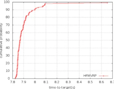
In the second experiment, time-to-target plots (TTTplots) (Feo & Smith, 1994) were performed to check the efficiency of the

GILS-VND

algorithm in reaching the solution currently used by the company. TTTplots display the probability (the ordinate) that an al-gorithm will ﬁnd a solution at least as good as a given target value within some given running time (the abscissa). TTTplots are also used byRibeiro and Resende (2012)as a way to characterize the running times of stochastic algorithms for combinatorial optimization.

(8)

Fig. 5.Time-to-Target Plot - HFMVRP_1.

Table 4

Company’s ﬂeet composition.

Veh. type Cap. Avail. MT Costs (in € )

(t) (qt) (mt) cft cct cdt

a 222 8 No 88.30 8 0.2446

b 414 5 No 115.70 8 0.3195

c 482 139 Yes 123.29 8 0.3315

d 550 3 No 148.87 8 0.3315

e 616 6 No 172.23 8 0.364

f 676 3 No 178.92 8 0.364

g 752 4 No 187.39 8 0.364

h 1,210 1 No 238.46 8 0.364

have been widely used as a tool for algorithm design and compari-son.

This experiment was run 100 times by the

GILS-VND

algorithm on a company instance with a total cost of € 32,472.37. This corre-sponds to instance K (seeTables 6and7). The execution ended once the algorithm found the target value (i.e., the same cost).Fig. 5shows the empirical probability curve. Note that our algorithm was able to ﬁnd the company solution in all experiments in less than 8.65 sec-onds. Based on this, we adopted a maximum computational time of 5 minutes in the experiments ofSection 5.3.

5.3. Benchmark results

To test the algorithm performance, we used 14 real instances that correspond to 14 different working days of the distribution company. We conducted two benchmark experiments: one to compare the per-formance of our algorithm and the

Rand-MER

algorithm by Caceres-Cruz et al. (2014), and the other to compare the results obtained by our algorithm with those obtained by the company. For the former, we considered the 10 instances presented inCaceres-Cruz et al. (2014, Table 4) (denoted by A, B, …, J), and for the latter, we considered five additional instances (denoted by K, L, … , O). The company distributes its products to 382 customers but it is frequent to have customers with zero demand for a particular day. This may be due to several reasons, for example, a store with low sales in the previous day that can wait another day to replenish, or a store that closes for a local holiday. The company has a fleet of 169 vehicles:Table 4shows the composition of this fleet by vehicle type, with its capacity (in boxes), the possibility of performing multiple trips, and the corresponding costs (fixed cost per vehicle, variable distance cost, and cost per cus-tomer visited, respectively).

Table 5

Results for real multi-trip instances:GILS-VNDvs.Rand-MER(distances in kilome-ter).

Rand-MER GILS-VND Differences

Instance #nCustomers Best Average Best Average Gap (%) Gap (%)

(1) (2) (3) (4) (3–1) (4–2)

A 372 39,534 39,841 38,995 39,572 −1.36 −0.68

B 366 41,072 41,399 40,670 41,243 −0.98 −0.38

C 371 49,669 50,082 46,116 49,639 −7.15 −0.89

D 364 31,378 31,543 31,300 31,600 −0.25 0.18

E 372 45,485 45,836 45,300 46,206 −0.41 0.80

F 373 45,275 45,681 42,100 44,942 −7.01 −1.64

G 372 45,165 45,493 44,983 45,883 −0.40 0.85

in 6 out of 10 instances.

(9)

Table 6

Comparison of results I:GILS-VNDvs.Company.

GILS-VND Company GILS-VND Company GILS-VND Company GILS-VND Company TC

Instance CF(€ ) CF(€ ) CC(€ ) CC(€ ) CD(€ ) CD(€ ) TC(€ ) TC(€ ) Gap (%)

Single trip

K 16,498 17,223 2944 2944 11,065 12,305 30,507 32,472 −6.05

L 8064 9117 2528 2528 5735 7353 16,327 18,997 −14.05

M 9174 10,066 2536 2536 6308 7665 18,018 20,266 −11.09

Multi-trip

N 25,815 29,543 2992 3032 16,716 19,075 45,523 51,650 −11.79

O 22,943 25,931 3008 3072 14,895 16,761 40,846 45,764 −10.62

Table 7

Comparison of results II:GILS-VNDvs.Company.

GILS-VND Company GILS-VND Company GILS-VND Company

Instance #nRoutes #nRoutes #nKm #nKm #nE #nE

SINGLE TRIP

K 134 134 33,403 36,733 1871 4533

L 66 71 17,601 22,185 894 4325

M 75 80 19,334 23,351 1003 3658

MULTI-TRIP

N 203/34 234/86 50,244 57,388 5420 19,164

O 181/12 205/56 44,639 50,423 3350 14,667

Table 8

Statistical results for the new set of instances:GILS-VNDvs.Company.

GILS-VND

Instance Company Best Average Std. dev. Gap (%)

K 32,472 30,507 30,692 70 −5.48

L 18,997 16,327 16,427 42 −13.53

M 20,266 18,017 18,146 43 −10.46

N 51,609 45,523 45,813 100 −11.23

O 45,764 40,846 40,995 66 −10.42

instances, the second number in the “#nRoutes” column represents the number of vehicles that performed two trips.

The

GILS-VND

algorithm was able to obtain cheaper solutions in all instances. The numbers reported belong to the best solution obtained by our algorithm in all the runs. These solutions represent savings on the operational costs of up to € 6,127 (e.g., Instance N), reducing ﬁxed vehicle costs by € 3,728 (i.e., using less vehicles) and traveling shorter distances (i.e., 7144 less kilometers in one day). Con-sidering that each instance corresponds to the distribution of a single day, the potential annual savings are considerable. In addition, our solutions are better with respect to all other routing indicators: less trips needed, less distance traveled, and vehicles with less residual capacity.

Next, we provide some statistical results on the total cost obtained by the algorithm for all 30 runs performed for the new set of ﬁve instances.Table 8shows these ﬁgures. The last column displays the percentage gap between the average algorithm solution and the com-pany solution, calculated as:

gapi=

TCGILSi −VND−TCiCOMPANY TCCOMPANY

i

(3)

whereTCi GILS−V ND

is the average algorithm solution andTCCOMPANY i is the company solution for instancei. In the worst case, the average cost is almost 6% better than the company solution.

6. Conclusions and extensions

Real vehicle routing problems present a variety of constraints that are sometimes disregarded in model formulations. These re-alistic constraints may have a signiﬁcant impact on the solution

implementation. This study analyzed a Heterogeneous Fleet Multi-trip VRP (HFMVRP) faced by a distribution company in Europe that serves around 400 customers. This real VRP variant considers a fleet of heterogeneous vehicles (i.e., vehicles with different capacities and costs) with the possibility of performing multiple trips or being un-able to serve particular customers (for maneuverability reasons, for example). The objective function included the company’s set of costs: a fixed cost per vehicle used, a variable vehicle cost per distance trav-eled and a fixed cost per customer visited. Due to the difficulty of the problem, we proposed a heuristic algorithm, the

GILS-VND, that

combines an

ILS, a

GRASP, and a

VND. The algorithm uses the power

of the

GRASP

to build a feasible initial solution, and then within the

ILS

structure, it uses the

VND

as local search combined with the Re-ﬁne method based on several levels of perturbation. With the use of smart mechanisms that discard solutions based on previous val-ues stored in ADSs, it was possible to enhance the solution reevalua-tion time in up to 98.90% for one of the real instances studied in this paper.

The authors are indebted to the two anonymous reviewers for their constructive suggestions that have helped us improve the orig-inal manuscript. This work has been partially supported byCNPq (grants552289/2011-6and306458/2010-1),FAPEMIG(grants PPM CEX497-13, APQ-04611-10), CAPES and Science Without Borders (grant 202380/2012-2 and 202381/2012-9), the Spanish Ministry of Economy and Competitiveness (TRA2013-48180-C3-P) and the Ibero-American Programme for Science, Technology and Develop-ment (CYTED2010-511RT0419)

References

Aiex, R. M., Resende, M. G. C., & Ribeiro, C. C. (2002). Probability distribution of solu-tion time in GRASP: An experimental investigasolu-tion.Journal of Heuristics, 8(3), 343– 373.

Aiex, R. M., Resende, M. G. C., & Ribeiro, C. C. (2007). TTTplots: A perl program to create time-to-target plots.Optimization Letters, 1(4), 355–366.

Amorim, P., Parragh, S., Sperandio, F., & Almada-Lobo, B. (2014). A rich vehicle routing problem dealing with perishable food: A case study.TOP, 22(2).

de Armas, J., & Melián-Batista, B. (2015). Variable neighborhood search for a dynamic rich vehicle routing problem with time windows.Computers & Industrial Engineer-ing, 85, 120–131.

Baldaccci, R., Battarra, M., & Vigo, D. (2008). Routing a heterogeneous ﬂeet of vehicles. In B. Golden, S. Raghavan, & E. Wasil (Eds.),The vehicle routing problem: Latest ad-vances and new challenges: 43(pp. 3–27). Springer.

Baldacci, R., & Mingozzi, A. (2009). A uniﬁed exact method for solving different classes of vehicle routing problems.Mathematical Programming, 120(2), 347–380. Belﬁore, P., Yoshizaki, Y., & Tsugunobu, H. (2009). Scatter search for a real-life

hetero-geneous ﬂeet vehicle routing problem with time windows and split deliveries in Brazil.European Journal of Operational Research, 199(3), 750–758.

Brandão, J. (2009). A deterministic tabu search algorithm for the fleet size and mix vehicle routing problem.European Journal of Operational Research, 195(3), 716–728. Caceres-Cruz, J., Grasas, A., Ramalhinho, H., & Juan, A. A. (2014). A savings-based ran-domized heuristic for the heterogeneous fixed fleet vehicle routing problem with multi-trips.Journal of Applied Operational Research, 6(2), 69–81.

Choi, E., & Tcha, D.-W. (2007). A column generation approach to the heterogeneous ﬂeet vehicle routing problem.Computers & Operations Research, 34(7), 2080–2095. Clarke, G., & Wright, J. W. (1964). Scheduling of vehicles from a central depot to a

num-ber of delivery points.Operations Research, 12(4), 568–581.

Coelho, I. M., Munhoz, P. L. A., Haddad, M. N., Coelho, V. N., Silva, M. M., Souza, M. J. F., & Ochi, L. S. (2011). A computational framework for combinatorial optimization prob-lems. InVII ALIO/EURO workshop on applied combinatorial optimization: 3(pp. 51– 54).Porto

Coelho, V. N., Guimaraes, F. G., Reis, A. J. R., Coelho, B. N., Coelho, I. M., & Souza, M. J. F. (2014). A general variable neighborhood search heuristic for short term load fore-casting in smart grids environment. InProceedings of the Power systems conference (PSC), 2014 Clemson University(pp. 1–8).

Coelho, V. N., Souza, M. J. F., Coelho, I. M., Guimaraes, F. G., Lust, T., & Cruz, R. C. (2012). Multi-objective approaches for the open-pit mining operational planning problem. Electronic Notes in Discrete Mathematics, 39, 233–240.

Dantzig, G. B., & Ramser, J. H. (1959). The truck dispatching problem.Management Sci-ence, 6(1), 80–91.

Dayarian, I., Crainic, T. G., Gendreau, M., & Rei, W. (2015). A column generation approach for a multi-attribute vehicle routing problem.European Journal of Operational Re-search, 241(3), 888–906.

Feo, T. A., & Resende, M. G. C. (1995). Greedy randomized adaptive search procedures. Journal of Global Optimization, 6(6), 109–133.

Feo, T. A., & Smith, M. G. C. R. S. H. (1994). A greedy randomized adaptive search proce-dure for maximum independent set.Operations Research, 42(5), 860–878. Gendreau, M., Laporte, G., Musaraganyi, C., & Taillard, E. D. (1999). A tabu search

heuris-tic for the heterogeneous ﬂeet vehicle routing problem.Computers & Operations Research, 26(12), 1153–1173.

Golden, B., Assad, A., Levy, L., & Gheysens, F. (1984). The ﬂeet size and mix vehicle routing problem.Computers & Operations Research, 11(1), 49–66.

Imran, A., Salhi, S., & Wassan, N. A. (2009). A variable neighborhood-based heuristic for the heterogeneous ﬂeet vehicle routing problem.European Journal of Operational Research, 197(2), 509–518.

Jiang, J., Ng, K. M., Poh, K. L., & Teo, K. M. (2014). Vehicle routing problem with a het-erogeneous ﬂeet and time windows.Expert Systems with Applications, 41(8), 3748– 3760.

Kritikos, M. N., & Ioannou, G. (2013). The heterogeneous ﬂeet vehicle routing problem with overloads and time windows.International Journal of Production Economics, 144(1), 68–75.

Laporte, G. (2009). Fifty Years of Vehicle Routing.Transportation Science, 43(4), 408– 416.

Leung, S. C., Zhang, Z., Zhang, D., Hua, X., & Lim, M. K. (2013). A meta-heuristic algorithm for heterogeneous ﬂeet vehicle routing problems with two-dimensional loading constraints.European Journal of Operational Research, 225(2), 199–210.

Li, F., Golden, B., & Wasil, E. (2007). A record-to-record travel algorithm for solving the heterogeneous ﬂeet vehicle routing problem.Computers & Operations Research, 34(9), 2734–2742.

Liu, S., Huang, W., & Ma, H. (2009). An effective genetic algorithm for the ﬂeet size and mix vehicle routing problems.Transportation Research Part E: Logistics and Trans-portation Review, 45(3), 434–445.

Lourenço, H. R., Martin, O. C., & Stützle, T. (2003). Iterated local search. In F. Glover, & G. Kochenberger (Eds.),Handbook of metaheuristics(pp. 321–353). Boston: Kluwer Academic Publishers.

Mladenovi ´c, N., & Hansen, P. (1997). Variable neighborhood search.Computers & Oper-ations Research, 24(11), 1097–1100.

Ochi, L. S., Vianna, D. S., Drummond, L. M. A., & Victor, A. O. (1998). An evolution-ary hybrid metaheuristic for solving the vehicle routing problem with heteroge-neous ﬂeet. InProceedings of the first European workshop, EuroGP’98: 1391(pp. 187– 195).Paris, France

Or, I. (1976).Traveling salesman-type combinational problems and their relation to the logistics of blood banking. USA: Northwestern University Ph.D. thesis.

Penna, P. H. V., Subramanian, A., & Ochi, L. S. (2013). An iterated local search heuristic for the heterogeneous ﬂeet vehicle routing problem.Journal of Heuristics, 19(2), 201–232.

Prins, C. (2002). Efficient heuristics for the heterogeneous ﬂeet multitrip VRP with application to a large-scale real case.Journal of Mathematical Modelling and Algo-rithms, 1(2), 135–150.

Prins, C. (2009). Two memetic algorithms for heterogeneous ﬂeet vehicle routing prob-lems.Engineering Applications of Artificial Intelligence, 22(6), 916–928.

Resende, M. G. C., & Ribeiro, C. C. (2010). Greedy randomized adaptive search pro-cedures: Advances, hybridizations, and applications. In M. Gendreau, & J. Potvin (Eds.),Handbook of metaheuristics(pp. 283–319). New York: Springer.

Ribeiro, C. C., & Resende, M. G. C. (2012). Path-relinking intensiﬁcation methods for stochastic local search algorithms.Journal of Heuristics, 18(2), 193–214.

Ribeiro, G., Desaulniers, G., Desrosiers, J., Vidal, T., & Vieira, B. (2014). Efficient heuris-tics for the workover rig routing problem with a heterogeneous ﬂeet and a ﬁnite horizon.Journal of Heuristics, 20(6), 677–708.

Souza, M., Coelho, I., Ribas, S., Santos, H., & Merschmann, L. (2010). A hybrid heuristic algorithm for the open-pit-mining operational planning problem.European Journal of Operational Research, 207(2), 1041–1051.

Stützle, T. (2006). Iterated local search for the quadratic assignment problem.European Journal of Operational Research, 174(3), 1519–1539.

Subramanian, A., Uchoa, E., & Ochi, L. S. (2013). A hybrid algorithm for a class of vehicle routing problems.Computers & Operations Research, 40(10), 2519–2531. Tütüncü, G. Y. (2010). An interactive gramps algorithm for the heterogeneous ﬁxed ﬂeet

vehicle routing problem with and without backhauls.European Journal of Opera-tional Research, 201(2), 593–600.