Welfare cost of inflation with heterogeneous agents

.... ｾｆｕｎｄａￇￃｏ＠

.... GETULIO VARGAS EPGE

Escola de Pós-Graduação em Economia

"Welfare Cost of Inflation with

Heterogeneous Agents"

Prof. Mirta Bugarin (UnB)

LOCAL

Fundação Getulio Vargas

Praia de Botafogo, 190 - 10° andar - Auditório

DATA

08/04/99 (58 feira)

HORÁRIO

Welfare Cost of Infiation with Heterogeneous

Agents

Mirta N. S. Bugarinl

Departamento de Economia Universidade de Brasília

April 1998

1 Introd uction

The common believe that inflation is the most regressive form of taxation is widely accepted and appears to be supported by empirical evidence. The welfare costs and the distributive impacts of inflation have not yet been studied in a general equilibrium framework with heterogeneous agents.

Defining the inflation tax as the revenue raised by the government through seigniorage, the average annual growth rate of 16.13% (1980), 47.41% (1985) and 146% (1990) of the monetary concept MI' reported by the Brazilian Central Bank, clearly represent an inflationary bias for revenue raising in Brazil.

Recent studies by Barros and Mendoça (1995), Mendoça and Urani (1994), Bonelli and Ramos (1994) among others, clearly show the alarmingly high leveI of income concentration in Brazil that had increased dramatically over the last 30 years. In particular the latter authors reveal a striking fact that despite the substantial upgrade in the educationallevel of the Brazilian labor force during the period 1977-1989 2, the concentration of income had been

rising. This suggests that there is no systematic way that education could have afIected the dynamic patter of the Brazilian income distribution as the theory of human capital formation would explain. An important insight from

lThe author is deeply grateful to Gary Hansen, Anne Villamil, Maurício Bugarin and Rolando Guzmán for their valuable suggestions and to Pedro Ferreira and Carlos Araújo for their help in gathering paramenter values. None of them is responsible for errors or opinions expressed.

2During this period the share of workers with less than intermediate schooling went down from 59% to 44% and the share of those that at least started attending high school increased from 19% to 29%

their research, however, is that the variable position in occupation 3, which is

closely related to ones's degree of control over capital, accounts for the high-est contribution in the variation of the Theil T index of inequality. Hence, the ownership of capital appears to be an important means of protecting in-come from inflation in Brazil. This strongly suggests that inflation could be the driving force behind the worsening of the Brazilian income distribution. The present study is based on the definition of recursive competi tive equilibrium (RCE) for a heterogeneous agents model as suggested by Hansen and Prescott (1995). The agents of the model economy are divided in two types, type 1 capital owners and type 2 employees, to match the model with the Brazilian empirical evidence. According to the RCE definition, a linear quadratic (LQ) approximation of the return function is numerically computed around the steady state variable values for each type of agent. This enables to translate the agent's problem into a LQ dynamic programing framework. Iterating simultaneously over the LQ value functions, a set of consistent and optimal (linear) decision rules and the aggregate pricing function are derived from the first order conditions.

This study has four goals. First, to quantitatively asses the impact of the inflation tax on aggregate welfare as well as on the income distribution based on a general equilibrium model economy with heterogeneous agents, calibrated for the Brazilian economy, in which money is introduced via cash-in-advance constraint. Second, to compare the outcomes of the inflation tax regime with alternative revenue neutral tax policy schemes. Policy 1 replaces the seigniorage revenue by increasing the tax rates on labor and capital in-come keeping a constant relationship between them, Policy 2 institutes an increase only on labor income, Policy 3 substitutes the inflation tax by an in-crease on capital income tax only and Policy 4 consists of levying an uniform tax rate on both sources of income. Third, to analyze the transition path to the steady state implied by the optimal decision mIes and the pricing func-tion associated with the RCE. Finally, to compare the effects of temporary vs. permanent policy changes in terms of welfare and equity.

The main findings show the regressive nature of the inflation tax and an apparent trade off between Pareto superior and equity improving pol-icy choices. Furthermore, the patterns of the transition paths (which are

obviously policy dependent) display a noticeable dominance of sequences de-rived from permanent tax policies relative to those obtained from temporary changes in policy.

The article is organized as follows. Section 2 describes the standard model economy with heterogeneity introduced based on the Brazilian empirical ev-idence on position in occupation (heterogeneous) groups. Section 3 presents the computational procedure used to find a recursive competitive equilibrium for the model economy based on the algorithm introduced by Hansen and Prescott (1996). Section 4 introduces the parameterization used to calibrate the mo dei economy and the obtained results. Section 5 contains concluding remarks.

2

The Model

According to Bonelli and Ramos (1994) the variable "position in occupation" divides the Brazilian work force among employees 75%, self employers 20% and employers 5%. These shares are shown to be constant over the period 1977-1989. To introduce this fact in a model economy with infinitely lived heterogeneous agents, let i = 1, 2 denote the groups such that type i = 1 agents control (own) capital, representing the self employers and employers, whereas type i = 2 agents do not have access to capital ownership, repre-senting the employees. In other words, type 1 agents supply labor h1 and accumulate productive capital k1 that is rented to the firm and, type 2 agents

only supply labor h2 to the single firm that produces output according to a

constant return to scale technology.

There is also a government in the economy that supplies money (cur-rency), taxes labor and capital income, and transfers a lump-sum amount of currency to both types of households. Money is valued in this economy for it is required to purchase consumption goods.

Type 1 Agents' Problem.

Consider a large number of identical type 1 agents endowed with capital ko

in period O, one unit of time per period that can be spent working or enjoying leisure and money balances ml,O at period O. The problem of a representative agent of type 1 is to choose optimal sequences for consumption

{Clt},

labor

discounted utility is maximized subject to the per period budget, cash-in-advance constraint, and feasibility. Formally, a type 1 agent's problem is given by:

(1)

such that,

ml t+l mlt trt

Clt

+

Xlt

+ '

:S

(1 - tw)Wthlt

+

(1 - tk)rtklt

+

tkl5klt

+ -

+

-Pt Pt Pt

PtClt

:S

mlt

+

M1,t+l - M1,t

hlt

+

llt = 1, t

2:

O

The law of motion for capital formation is klt = (1-I5)k1,t-l

+

Xlt, the initial capital stock is k_o,

O

<

(3

<

1 is the discOlmt rate,

Clt is the consumption of type 1 agent at time t,

O

:S

hlt

:S

1 denotes the units of working time of type 1 agent,

Xlt denotes the type 1 agent's investment decision at time

t,

tw is the tax rate on labor income,

Wt is the wage rate at time t,

tk is the tax rate on capital income,

rt is the rate of return for capital services at time

t,

klt is the capital stock at time t held by type 1 agent,

15 is the capital depreciation rate, and

trt is the lump sum transfer from government at time t.

Type 2 Agents' Problem.

(2)

such that,

m2 t+l m2t trt

C2t

+ -'- :::;

(1-tw)Wth2t

+ -

+-ｾ＠ ｾ＠ ｾ＠

PtC2t :::; m2t

+

M 2,t+1 - M 2t

h2t

+

b

= 1, t:2:0

Note that hi and mi denote particular type í = 1,2 agent's labor choice and money holdings. Let Ài denote the proportion of type í = 1,2 agents such that À1

+

À2

=

1. The aggregate per capita variables are Kt

=

À1K1 for capital stock, Mt = ÀIMlt

+ À 2M 2t

for the pre-transfer money supply,

Ht = À1Hlt

+ À 2

H2t for total hours worked, and Xt

=

À1Xlt for aggregate

investment.

Observe that the budget constraint does not allow either type of agent to purchase or sell state-contingent claims to units of output next-period. AIso, consumption goods are only purchased in cash: agents enter period t with nominal balances mi,t which are augmented by a lump sum transfer of

newly printed money M i,t+l - Mi,t. Therefore, the (post-transfer) amount of

nominal money, the right hand si de of cash-in-advance constraint, is available at t to finance the purchase of "cash" good Ci,t.

The Governrnent

The per period (pre-transfer) money supply evolves according to the growth factor g. Therefore, given the price leveI Pt, the real inflation tax

revenue collected by the government is given by:

M t+1 - Mt (g - l)Mt

-Pt Pt

ｔｾ＠

M

- = TwwtHt

+

Tk(rt - 8)Kt

+

(g -1)- (3)

ｾ＠ ｾ＠

Moreover the following is assumed to hold for both types of agents:

Assumption 1 The period utility function u(.,.) : R+ -+ R is bounded, con-tinuously differentiable, strictly concave, strictly increasing in both arguments and satisfies the lnada conditions, i.e. (UdU2) -+ 00 as (ct!(1- ht)) -+ O and (UdU2) -+ O as (ct!(l- ht)) -+ 00. Hence both consumption and leisure are normal goods.

The Firm

The productive sector of this model economy hires labor

h{

and capital services

k{

at every t to produce output

y{,

according to a constant return to scale technology. Thus, without loss of generality it is assumed that there is only one firm, operating at zero profit using the technology given by:

(4)

where,

Zt : exogenous shock to the technology realized at time t.

Furthermore, the following is assumed:

Assumption 2 The technology shock described by Zt = eWt

, has a random

term Wt evolving according to the first order auto regressive process Wt = PWt-1

+

Et, O

<

P

<

1 and Et is i. i. d. with mean zero and finite variance

0";.

The term Wt captures the productivity shock which is the source of un-certainty for this economy.

The technology satisfies the following:

Assumption 3 The constant return to scale production function f ( ., .)

The per period wage rate Wt and the rate of return on capital rt are derived

from the first order conditions of the firm's profit maximization problem and are given by:

Wt = Zt!2(k{, h{)

(5)

(6)

Using market clearing conditions k{

=

KtN and h{

=

HtN, denoting the total number of households by N = À1N1

+

À₂N_{2 ,} the following equilibrium

conditions are obtained:

(7)

(8)

It is also assumed that the aggregate per capita capital stock evolves according to the law of motion given by:

(9)

In order to focus on stationary equilibrium for the households, the mon-etary variables are transformed4 _{in the following fashion:}

ｾ＠ mit d mit = Mt an ,

ｾ＠ Pt

Pt=-M '

t+l

such that real money balances becomes:

Pt Pt

4This transformation is needed because if the monetary growth factor is positive, i.e.

Introducing the transformed monetary variables and the government trans-fer by type of agent, problem (1) becomes for t ｾ＠ O:

(10)

such that,

XIt+

m1;t+l :::;

Wt(hlt+tw(HIt - hIt)+rt(klt+tk(KIt - kIt )) +btk(kIt - K lt ) Pt

(mlt - M1,t) M1,t+l Clt :::; A

+

A •

Pt9 Pt

Similarly, problem (2) becomes for t ｾ＠ O:

(11)

such that,

(m2t - M2,t) M2,t+l C2t :::; A

+

A •

Pt9 Pt

Solving the respective budget constraints for hit , t = 1,2, and aggregating

over each type of agent, expressions for Hit, i = 1,2 are obtained. Aggre-gating once more over both types of agents _Ht

=

ÀIHl

+

(1 - _À1)H2. The following symbolic expression is derived:

H = ( XltPt À

+

1 )

1':'0

t Zt (À1Klt)(}pt

Substituting above expression into Hit , the latter is used to find the

func-tions hlt = hIt(z, Kl' k1, Mlt,pt) and h2t = h2t(z, Kl' M2t ,pt) that enter the utility function, where Wt = zth(À1Klt , Ht), rt = Zdl (>'lKt, Ht ) from the

firm's profit maximization condition and, Cit, i = 1,2 are obtained from the cash-in-advance constraint.

describing the entire distribution of the capital stock, hours worked, invest-ment and money balances over type i = 1,2 agents. The agents' optimization problem can now be expressed as the dynamic programing problem below.

For type 1 agents:

subject to:

z'

=

pz

+

f.'

ｫｾ＠ = (1 - 8)kl

+

Xl

ｋｾ＠ = (1 - 8)KI

+

Xl

Xl = X1(z,K)

HI = H1 (z,K)

M{

= ｍｾＨｺＬｋＩ＠

For type 2 agents:

v2(z,K)

=

ｭ｡ｸｻｲＲＨｺＬｋＬｭＲＬｘＬｍＧＬｭｾＬｰＩ＠

+

ＬＶｅ｛ｶＨｺＧＬｋＧＬｭｾＩＯｺ｝ｽ＠ (13)

subjed to:

z'

=

pz

+

f.'

K{

=

(1 - 8)KI

+

Xl H2 = H2(z,K)

ｍｾ＠ =

MHz,K)

The last three equation indicate that for each type of agent hours worked and money balances are functions of the state of the economy described by the productivity shock z and the vedor K of distribution of capital stock across the economy.

Definition of Recursive Competitive Equilibrium (RCE)

According to Hansen and Prescott(1995) a RCE is defined as follows:

(i) A set of decision roles: For type 1 agent:

Xl = Xl (z, K, k1 )

ｭｾ＠ = ｭｾ＠ (z, K, k1 )

For type 2 agent:

m;

= m;(z,K)

(ii) A set of aggregate decision rules, for i = 1,2:

li = li(Z, K)

1M;

= Mi(Z,K)

(iii) A function determining the aggregate price level:

fi

= P(z, K) and,

(iv) A set of value functions Vi(Z, K), i = 1,2 such that:

1. Given the decision roles in (i) and the aggregate price function in

(iii) , the value function Vi satisfies the value function (12)/(13) above and, (ii) are the associated decision roles.

and,

2. Given the pricing function in (iii) , individual decisions are con-sistent with aggregate outcomes, i.e. for i = 1,2:

ll(Z,K) = xl(z,K,KI )

M;(z, K) = ｭｾＨｺＬ＠ K), i = 1,2.

where _{￀ｉｍｾ＠} (z, K)

+

(1 - ￀ｬＩｍｾＨｺＬ＠ K) = 1, because by definition

1M;

represents type i agent's aggregate per capita money holdings relative to aggregate per capita money supply.

3

Computational Procedure

In order to numerically solve for the above defined RCE, the method proposed by Hansen and Prescott (1995) is implemented as follows.5

Step 1. Computation of steady state values.

Step 2. Assume the functional form Uit = CdOg(Cit

+

(1 - a)log(l - h_{it ),} i = 1,2 for the utility function and a Cobb-Douglas production function

f(zt, Kt, H_t) = ztKf H(l-B) ,the return function of problems (12) and(13) are

approximated numerically by the first three terms of the Taylor series expan-sion around the variables' steady state values to obtain the negative semi-definite matrices Qi, i

=

1,2, in order to express the problems in a linear quadratic programing framework, Le.:

For type 1 agents:

VI (z, K)

=

ｭ｡ｸｻｹｾ＠ QIYl

+

,BE[v(z', K')/z]} (14)

subject to:

z' = pz

+

E'

ｫｾ＠ = (1 - ó)kl

+

Xl

ｋｾ＠ = (1 - Ó)KI

+

Xl

Xl = X1(z,K) HI = H1(z,K)

M{

= ｍｾＨｺＬｋＩ＠

where YI

=

_{ＨｚＬｋｉＬｫｬＬｍｉＬｭｬＬｘｉＬｸｉＬｰＬｍｻＬｭｾＩ＠}

For type 2 agents:

subject to:

z' = pz

+

E'

ｋｾ＠ = (1 - ó)KI

+

Xl H2 = H2(z,K)

ｍｾ＠ = ｍｾＨｺＬｋＩ＠

where Y2 = (z, KI' M2' m2, XI,p, ｍｾＬ＠ ｭｾＩ＠

(15)

Step 3. Successive approximations of the value function are performed

simultaneously for both types of agents iterating on the mapping below:

11

subject to:

Z' = PZ

+

E'

ｫｾ＠ = (1 - ó)kl

+

Xl

ｋｾ＠ = (1 - Ó)KI

+

Xl Xl = Xl (Z, K) and,

Hi = Hi(z,K)

M;

=

M[(z,K), i

=

1,2

(16)

Step 4 When the above iterations have converged, the associated optimal

(linear) decision rules and pricing function are obtained, Le. For type 1 agent:

X I (z,KI ,MI ) = xI(z,KI,KI,MI,Ml) M{(z, KI' M I ) =

ｭｾＨｺＬ＠

KI' Kl' MI' M I )

For type 2 agent:

ｍｾＨｺＬ＠

KI' M 2) =

ｭｾＨｺＬ＠

KI' M2' M2 )

Observing the restriction À_I

M

₁

+

(1 - À_I)M₂ = 1 and,

fi

= P(Z,KI)

4

Results

The parameter values, in a quarterly bases, used to compute the RCE of the standard model are as follows:

Technology parameters:

e

=

0.4908, Ó

=

0.0168, P

=

0.78 and (JE

=

0.0016.

Preferences parameters:

f3

=

0.9835 and a

=

0.5885. Tax policy parameters:

9

=

1.0403, tw

=

0.2553 and, tk

=

0.3379.

Solow residual using real quarterly GNP and labor input data from Indi-cadores IBGE (1974-1991), assuming quarterly variation in capital stock to be approximately zero.

Preference parameters were also been estimated by Araújo (1997) and here are adjusted to quarterly bases. Among the tax policy parameters, the tax rate on labor in come as welI as capital income, tw and tk, were obtained

as the average of the progressive tax rates based on data from Secretaria da Receita Federal (1995). The money supply growth factor 9 was computed as the quarterly average growth of M1 based on data from Boletim do Banco

Central do Brasil, taking 1980 as the base year.

4.1

Steady State Analysis

The steady state variable values of the standard model (S.M.) economy with heterogeneous agents as welI as the simulated model with different tax poli-cies are reported in Table ?? AlI policies are revenue neutral. When the inflation tax is eliminated the foregone revenue is replaced by either of the folIowing tax regimes.

Policy 1 (P.l.) refers to a tax policy in which the relation between the two income tax rates tw and tk were kept constant. Eliminating the infiation

tax implied an increase in both tax rates, on labor income to

t;

= 0.2899 and

tl

= 0.3837.

With Policy 2 (P.2.), the inflation tax was substituted by an increase on1y in the labor income tax rate, the latter increases in this case 23.97% to

t!

= 0.3165.

Policy 3 (P.3.) replaces the infiation tax in a revenue neutral way increas-ing on1y the capital income tax rate to

tZ

= 0.4435.

Policy 4 (PA.) institutes an uniform tax rate over alI sources of income. This policy implies an increase in the tax rate on labor income of 27.03% and an decrease in the tax rate on capital income of 4.02%, leading to an uniform tax rate on income of

tu

= 0.3243.

Table 2 shows the aggregate per capita steady state variable values, cor-responding to the homogeneous agent models for the standard as welI as the simulated economies with alternative tax policies.

Table 1: Steady State Variable Values - per (type) capita

Varo Kl Xl Hl H2 Ml M2 Cl C2

S.M. 193.3058 3.2475 0.0520 0.5017 1.5522 0.8160 5.1804 2.7229

P.1. 175.3948 2.9466 0.0406 0.4997 1.5598 0.8134 4.9859 2.6000

P.2. 187.8765 3.1563 0.0430 0.4902 1.5395 0.8202 4.9936 2.6602

P.3. 157.7802 2.6507 0.0366 0.5116 1.5868 0.8044 4.9353 2.5020

PA. 191.3821 3.2152 0.0435 0.4873 1.5335 0.8221 4.9912 2.6756

Table 2: Steady State Variable Values (aggregate per capita)

Varo K X H C Y

S.M. 48.3264 0.8119 0.3893 3.3373 4.1492 PI. 43.8487 0.7367 0.3849 3.1964 3.9331 P2. 46.9691 0.7891 0.3784 3.2436 4.0326 P3. 39.4451 0.6627 0.3828 3.1103 3.7730 P4. 47.8455 0.8038 0.3763 3.2545 4.0583

4.1.1 Welfare Analysis

Based on the results presented in the tables above, an aggregate per capita welfare measure is constructed as the weighted sum of the heterogeneous agents' utilities, Le. W P = ÀlUl

+

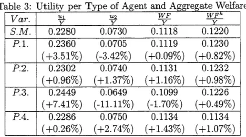
(1-_{À l )U2.} Table 3 presents in column (1) the leveI of per capita aggregate output and columns (2) to (5) introduce the aggregate per capita utility and welfare measures in terms of the aggregate per capita output, where W ph refers to the welfare measure corresponding to the homogeneous agents model.

Measured in terms of per capita aggregate output, the welfare measure improves if the infiation tax is replaced in a revenue neutral way by any of the alternative tax policies except for policy 3 which increases the tax rate on capital income only. It is also interesting to observe that in the model with homogeneous agents, policy 3 also leads to an improvement in welfare in terms of output. Moreover, with policies 2 and 4 the heterogeneous agents

fi

Table 3: Utility per Type of Agent and Aggregate Welfare

Varo !!:l.

_v

ｾ＠_y WF WF"

Y Y

S.M. 0.2280 0.0730 0.1118 0.1220

P1. 0.2360 0.0705 0.1119 0.1230 (+3.51%) (-3.42%) (+0.09%) (+0.82%)

P2. 0.2302 0.0740 0.1131 0.1232 ( +0.96%) (+1.37%) (+1.16%) (+0.98%)

P3. 0.2449 0.0649 0.1099 0.1226 (+7.41%) (-11.11%) (-1.70%) (+0.49%)

P4. 0.2286 0.0750 0.1134 0.1134 (+0.26%) ( +2.74%) (+1.43%) (+1.07%)

model displays a greater improvement in terms of aggregate welfare than the homogeneous agents model. Conversely, the former model shows a smaller improvement in welfare with policy 1.

In aggregate per capita bases, policy 4 shows the best welfare improve-ment of 1.43%. Policy 2 leads to the second best improveimprove-ment of 1.16% followed by policy 1. Implementing policy 3 leads to a deterioration in the welfare measure. In the homogeneous agents model, the best policy in terms of welfare improvement is still policy 4 but the increase in welfare is only 1.07%, 25% less than the improvement in the heterogeneous agents model. Surprisingly, all other policies, including policy 3, show an improvement in welfare.

in Tables 1 and 2.

4.1.2 Income Distribution Analysis

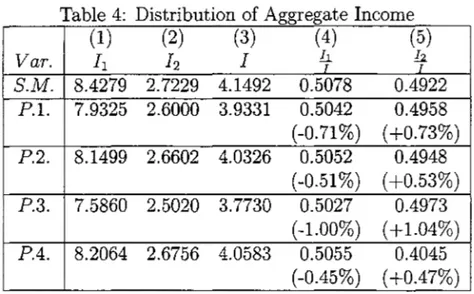
The interesting feature of using an heterogeneous agents mo deI is permits the analysis of distributive questions. The table below reports the (per capita -per type) aggregate income in columns (1) and (2), the aggregate -per capita income in column (3) and the relative participation of each type of agent in aggregate in come in columns (4) and (5), for the standard as well as the simulated policy models.

Table 4: Distribution of Aggregate Income

(1) (2) (3) (4) (5)

Varo 11 12 1

l;-

I;

S.M. 8.4279 2.7229 4.1492 0.5078 0.4922

P1. 7.9325 2.6000 3.9331 0.5042 0.4958 (-0.71 %) (+0.73%)

P2. 8.1499 2.6602 4.0326 0.5052 0.4948 (-0.51%) (+0.53%)

P3. 7.5860 2.5020 3.7730 0.5027 0.4973 (-1.00%) (+1.04%)

P4. 8.2064 2.6756 4.0583 0.5055 0.4045 (-0.45%) (+0.47%)

From the last two columns (4) and(5) it is clear that the elimination ofthe inflation tax in a revenue neutral way by either of the considered income tax schemes improves the distribution of income between the two types of agents, characterizing the inflation tax as a regressive distributive mechanism.

The above table shows that from the perspective of equity, policy 3 brings the best distributive outcome at steady state, leading to an increase of 1.04% in the participation of type 2 agents in aggregate income. Policy 1 which keeps a constant ratio between the two income tax rates relative to the stan-dard model economy presents the second best distributive resulto

a revenue neutral fashion, both types of agents would choose either policy 2 or 4 as they are the Nash equilibrium of such a game. Furthermore, if perfect coordination between the agents is assurned, either policy could be implemented, leading to an improvement in the welfare-output ratio for both types of agents as well as in the equity of income distribution.

4.2 Transition Path

The optimal investment decision rule as well as the corresponding pricing function, as functions of the state variables z and

K,

were derived for the homogeneous agents model solving the analog to problem (14) observing that in equilibriurn

M

= 1. This is introduced in Table below along with the cor-responding optimal rules as well as the pricing function for the heterogeneous agents models, the solution to problems (14) and (15). 6

Aggregating over both types of agents, Kt = ÀIKlt, Lt = ÀILlt

+

(1 -À1)L2t , Ct = ÀIClt+(1-Àlt)C2t, the main statistics ofthe obtained sequences are reported in Table 6 in aggregated per capita terms, together with the transition path implied by the homogeneous agents model over a period of 100 quarters.

As suggested by the Table ??, the introduction of two different types of agents into the model economy increases the variance of the sequence for all considered variables even though the mean values are very dose to each other. The representative agent's modelleads to a faster approximation to the corresponding steady state values but also generates a per capita welfare path that is consistently higher than the welfare sequence implied by the heterogeneous agents model. This result suggest that the used heterogeneous agents model captures a consistently lower welfare-output path due to the infiation taxo

Computing, within the heterogeneous agent framework, the capital stock (per type 1 capita) path, the optimallabor choice sequence, the consurnption path and the utility path by type of agent over a period of 25 years, it can be seen, as expected, that the consumption and utility values for type 1 agents who have two sources of income are higher than for type 2 agents, whereas the optimal labor choice is consistently higher for type 2 agents, for labor is

Table 5: Optimal Decision Rules

Homogeneous Agents Model Optimal Investment Decision Rule

X t

=

aà

+

a?Zt

+

｡ｾｋｴ＠

aa ｡ｾ＠ aq

29.2945 -0.0010 -0.5894 Pricing Function

A h h hK

Pt

=

Co

+

CI Zt

+

C2 t

ca

ｃｾ＠

cq

-16.2796 -6. 1162e-04 0.3431 Heterogeneous Agents Model Optimal Investment Decision Rule

X t

= ao

+

alZt

+

a2Kt

ao aI a2

49.4318 1.6172 -0.2473

Optimal Money Holding - Type 1 RA JVht

=

blO

+

bll Zt

+

bI2Kt

blO bll bI2

554.4837 -2.2344 -2.8488 Optimal Money Holding - Type 2 RA

Mlt

=

b20

+

b2I Zt

+

b22Kt

b20 b2I b22

-183.4920 0.7448 0.9496 Pricing Function

Pt

=

CO

+

CIZt

+

C2Kt

Co CI C2

24.6439 -0.1947 -0.1249

the only source of income for them. The sequences corresponding to type 1 agents follow the endogenously determined capital stock cycle.

Table 6· Transition Path Statistics

Varo Mean(Hom.) Std(Hom.) Mean(Het.) Std(H et.)

Capital Stock 48.3262 0.0037 48.3267 0.0089

Labor 0.3889 0.0052 0.3888 0.0096

Consumption 3.3396 0.0188 3.3388 0.0557

Welfare 0.5070 0.0026 0.4620 0.0099

transition path can be analyzed using the optimal rules and the pricing func-tions depicted in the following Table 7.7

Table 7: Heterogeneous Agents Model

Optimal Investment Decision Rule Xt

=

ao

+

alZt

+

a2Kt

ao aI a2

P.2 31.9709 0.1752 -0.1543

Po4 61.9053 0.1394 -0.3074 Optimal Money Holding Rule Ag.l:

Mlt

=

blO

+

bnZt

+

bI2Kt Ag.2: M2t

=

b20

+

b21Zt

+

b22Kt

blO bn b12

P.2 -57.0703 -0.0452 0.3122

Po4 -4004263 -0.0854 0.2197

b20 b2I b22

P.2 20.3568 0.0151 -0.1041

Po4 14.8028 0.0285 -0.0732 Pricing Function

Pt

=

CO

+

CIZt

+

C2 K t

Co CI C2

P.2 -281.7900 -004603 1.5040

Po4 -192.2403 -004323 1.0083

Transition Path of Alternative Tax Policies, t=l, ... ,lOO.

Analysing the transition paths for aggregate welfare in terms of aggregate output, the revenue path, the optimallabor sequence and the aggregate per capital stock path, respectively, for the basic model, tax policy 2 and tax policy 4 for an interval of 100 quarters, it can also be seen that policy 2 generates paths for aggregate per capita revenue, labor and capital stock consistently lower than the ones implied by the standard mo deI and by policy 4. In terms of aggregate per capita welfare-output sequence this policy Pareto dominates the others only after t

=

18.

If for equity criteria the per capita-per type income participation in terms of aggregate per capita income is considered, the implementation of policy 4 presents a more equitable distribution of income. The corresponding mean participation is 0.5071 for type 1 agents and 0.4929 for type 2 agents and its standard deviation is 0.0127 over the same interval.

Therefore, the above results suggest that if what matters for the model economy is an equitable distribution of income between type 1 and type 2 agents, policy 4 which institutes an uniform tax rate over both capital and labor income, would be the most desirable policy choice, although the implementation of this policy leads to a lower welfare-output ratio than the alternative policy 2 after period t = 18.

Policy Changes After t=lO.

Assume now that the economy starts as the standard model economy with an inflation tax and from period t = 10 one of the alternative NE tax policy scheme is implemented. In this case, as is expected, policy 4 (the uniform tax rate regime) will bring about a higher leveI of revenue, capital stock and labor choice after t = 10 than policy 2 (which increases only the tax rate on labor income). In terms of the welfare-output ratio, this result is true only up to t = 20 along the first 10 periods of policy implementation after which policy 4 results in a consistently lower leveI of aggregate welfare reI ative to aggregate output.

income participation (0.4879 for type 2) with a standard deviation of 0.0439 which represent a better outcome from an equity standpoint compared to a mean of 0.5575 for type 1 agent's income participation with a higher standard deviation of 0.1079 associated with the path generated with policy 2.

Temporary Policy Changes

Another exercise is performed based on a common fact that so called "stabilization policies" are often temporary. Then, the natural step is to analyze the transition path implied by these unexpected temporary policy changes, for it is assumed to be a "surprise" from the agent's point of view.

As should be expected, the transition paths over an interval of 50 periods (12.5 years) in which either policy 2 or policy 4 are implemented temporarily for 10 quarters (2.5 years) show that the revenue path follows a combination of labor and capital sequences with policy 4 leading to a higher leveI of these variables over the time period 10 to 30. Moreover, the labor path implied by both policies moves in opposite direction to each other. Policy 2 levies a heavier burden on labor income and has a negative impact on the decision to work (hence on the associated revenue path). The aggregate welfare-output ratio presents a different pattern with policy 4 reflecting a faster adjustment to the temporary change in policy than the alternative policy 2 regime.

In order to analyze the impact on income distribution caused by such a temporary policy change compared to a permanent elimination of the infla-tion tax, Table 8 reports the main comparative statistics of the respective sequences taking into consideration their first 50 periods.

Comparing the temporary vs. the permanent policy implementation, the results strongly suggest that cutting down the inflation tax only for 10 quar-ters (2.5 years), with either policy 2 or policy 4, leads to a worse distribution of income over the considered 12.5 years, both in terms of the mean value as well as of the standard deviation of the sequences. If a permanent policy change is to be implemented, policy 4 appears to be more desirable from a distributive point of view leading to a mean income participation of 0.5230 for type 1 agents (0.4770 for type 2 agents) compared to 0.6038 for type 1 agents (0.3962 for type 2) brought about by a permanent change to policy 2.

Table 8· Permanent vs. Temporary Policy Changes Main Statistics, t=1:50.

Policy 2

Permanent Temporary

Mean St. Dev. Mean St. Dev.

!lo 0.6038 0.1383 0.6327 0.1819

l.

_I 0.3962 0.1383 0.3673 0.1819 Policy 4

Permanent Temporary

Mean St. Dev. Mean St. Dev.

!lo _0.5230 0.0604 0.5658 0.1233

l.

-T 0.4770 0.0604 0.4342 0.1233

implementation of policy 2 for the considered time span.

5

Conclusion

Summarizing the main findings, when comparing the inflation tax policy rel-ative to the other alternrel-ative tax policy schemes, the steady state analysis has clearly shown the relevance of using a heterogeneous agents model within a RCE approach. In terms of the aggregate welfare-output ratio, any simu-lated alternative tax policy to the inflationary model economy, using a RA's model, results in a mild improvement of up to 1.07%. With a heterogeneous agents model, this welfare enhancing effect attains an improvement of up to 1.43% except with policy 3.

It is also shown that from an equity point of view, all alternative rev-enue neutral tax regimes are desirable compared to the income distribution outcome of the inflation tax scheme. Income equality improves most with policy 3 which increases only the tax rate on capital income. Hence, the trade-off between equity and efficiency becomes apparent: the policy that can improve the income distribution the most is Pareto dominated by the other alternative policies.

increases consistently only through policy 2 or policy 4 which constitute the two NE used to examine the dynamics of the transition path.

The transition path analysis over 100 time periods shows that the se-quences of the aggregate per capita variables implied by the optimal decision rules and the price function associated with the two (Nash) RCE describe a difIerent pattern depending on the timing and duration of the implemented policy.

If from a common arbitrary initial capital stock and productivity shock the obtained sequences are compared, policy 2 leads to a consistently higher (Pareto superior) leveI of aggregate welfare-output ratio after period t=18. If the alternative tax policies are implemented permanently from t=10 on, policy 4leads to a higher welfare-output ratio only from period t=10 to t=20, from which its path associated with policy 2 Pareto dominates the others.

In the case of a temporary decrease of the infiation tax, only from t= 10 to t=20, the aggregate per capita welfare in terms of aggregate output shows an immediate improvement which dominates policy 2's path over more than half of the temporary implementation period. The transitory nature of either policy leads to a sharp deterioration of approximately 0.75% of the welfare measure which can be recovered only after the following 10 periods.

Moreover, contrasting the distributive impact of temporary vs. perma-nent policy changes over the interval of 50 periods, the former has a negative impact on the income distribution for either policy reI ative to their perma-nent application.

This study constitutes an example of the relevance of heterogeneous agents models within a RCE framework to analyze both welfare and dis-tributive impacts of government revenue funding through an inflation taxo Furthermore, the dynamic nature of the RCE along with the linear quadratic algorithm allows one to derive explicitly the associated optimal decision rules. This is crucial for analyzing the transition path movements towards the steady state implied by the difIerent policy regimes.

References

[2] Banco Central do Brasil (1980-1992). Suplemento Estatístico.

[3] Bonelli, R. and Ramos, L. (1994). "Income Distribution in Brazil: an evaluation of long-term trends and changes in inequality since the mid-1970s", in Mendonça, R. and Urani, A. (org.) Estudos Sociais e da

Trabalho, IPEAjDIPES, VoI. 1, Rio de Janeiro.

[4] Barros, R. P. de and Mendonça, R. (1992). "A evoluç ão do Bem-Estar e da Desigualdade do Brasil desde a Década de 60", Texto para Discussão IPEAjDIPES, Rio de Janeiro.

[5] Cooley, T.F. (1995) Frontiers in Business Cycle Research. Princeton, N J: Princeton University Press.

[6] Cooley, T.F. and Prescott, E. (1995). Economic Growth and Business Cycles. In Cooley, T.F., editor, Frontiers in Business Cycle Research.

Princeton, NJ: Princeton University Press.

[7] Hansen, G.D. and Prescott, E. (1995). Recursive Methods for Comput-ing Equilibria of Business Cycle Models. In Cooley, T.F., editor, Fron-tiers in Business Cycle Research. Princeton, NJ: Princeton University Press.

[8] Hausman, J.A. (1985). Taxes and Labor Supply. In Auerbach, A.J. and Feldstein, M., editors, Handbook of Public Economics voI. 1. Elsevier Science Publishers B.V. (North-Holland).

[9] IBGE (1996). Indicadores IBGE. RJjBrasiI.

[10] IESP (1996). Indicadores IESP. SP jBrasiI.

[11]

Kydland, F. and Prescott, E. (1982). 'Time to Build and Aggregate Fluctuations', Econometrica 50:1345-1370.

[12] Mendonça, R. and Urani, A. (1994) (org.) Estudos Sociais e do Trabalho,

IPEAjDIPES, VoI. 1, Rio de Janeiro.

N.Cham. P/EPGE SPE B954w Autor Bugarin. Mirta Noemi Sataka.

Título Welfare cost of inflation with heterogeneous 088980

1111111111111111111111111111111111111111 52007

FGV - BMHS N° Pat.:F2697199