Stability of a half-sine shallow arch under sinusoidal and step loads in
thermal environment
Abstract
The complex structural behavior of shallow arches can be remarkably af-fected by many parameters. In this paper, the structural responses of a half-sine pin-ended shallow arch under sinusoidal and step loadings are accurately calculated. Additionally, the effects of environmental tempera-ture changes are considered. Three types of sinusoidal loadings are sepa-rately investigated. Displacements, load-bearing capacity, the magnitude of the axial force and the locus of critical points (including limit and bifurca-tion points) are directly obtained without tracing the corresponding equi-librium path. Furthermore, the boundaries identifying the number of criti-cal points are investigated. All mentioned structural responses are formu-lized based on the rise of the arch and the environmental temperature change, which are introduced in a dimensionless form. The proposed for-mulation is also developed for generalized sinusoidal loadings. Additional-ly, the structural behavior of the shallow arch under two types of step load-ings is investigated. Finally, the accuracy of the suggested approach is ex-amined by a non-linear finite element method.
Keywords
Half-sine shallow arch, equilibrium path, critical point, bifurcation, stability analysis.
1 INTRODUCTION
Shallow arches are widely used in structural, mechanical and aerospace engineering, and the investigation of structural stability has always been of the researchers’ interest. The failure of such structures is in the form of material failures, structural instability or a combination of them.
The tendency of structure to return to the static state, after creating a perturbation in the degrees of freedom, is called stability (Thompson and Hunt, 1973; Khalil, 2002). In the analysis of structural stability, since the struc-ture experiences the sudden deformations, the investigation of critical points (such as limit and bifurcation point) is crucial. Such deformations cause severe changes in strains and stresses. The geometry of the arch is an influen-tial parameter on its load-bearing capacity (Cai et al., 2012; Bateni and Eslami, 2015; Bradford et al., 2015; Re-zaiee-Pajand and Rajabzadeh-Safaei, 2016). In addition, various loadings (e.g., the sinusoidal (Plaut and Johnson, 1981), concentrated (Pi et al., 2008; Chandra et al., 2012; Tsiatas and Babouskos, 2017), distributed (Moghad-dasie and Stanciulescu, 2013b) and end moment loads (Chen and Liao, 2005; Chen and Lin, 2005)), geometric imperfections (Virgin et al., 2014; Zhou et al., 2015a), and boundary conditions (Pi and Bradford, 2012; Pi and Bradford, 2013; Han et al., 2016) are other important factors in the structural design.
In most cases, shallow arches become elastically unstable when the lateral load reaches a critical value (Chen and Li, 2006). This means that a large deformation could be observed while the material remains elastic. Practical experiences also confirm this issue (Chen and Liao, 2005; Chen and Yang, 2007a; Chen and Ro, 2009). Conse-quently, the behavior of shallow arches can be explained by the non-linear theory of elastic stability. In some analyses, it is assumed that the displacements of the arch are limited to avoid a material failure (Pippard, 1990; Xu et al., 2002; Chen and Hung, 2012). In addition, the variation in the environment temperature can be influen-tial on the stability of structures (Matsunaga, 1996; Hung and Chen, 2012; Stanciulescu et al., 2012; Kiani and Eslami, 2013).
Several approaches can be applied to investigate the structural behavior of shallow arches. Previously, both analytical and numerical methods are discussed in the literature (Plaut and Johnson, 1981; Reddy and Volpi,
Mohsen Saghafi-Nika
Behrang Moghaddasieb*
a Department of Civil Engineering Khorasan
Razavi Neyshabur, Science and Research Branch, Islamic Azad University, Neyshabur, Iran. E-mail: [email protected]
b Department of Civil Engineering, Ferdowsi
University of Mashhad, Mashhad, Iran. E-mail: [email protected]
*Corresponding author
http://dx.doi.org/10.1590/1679-78254607
1992; Pi et al., 2002; Xenidis et al., 2013). In some analytical techniques, the displacement field is replaced by a set of orthogonal functions to derive the non-linear equilibrium and buckling equations (Xu et al., 2002; Chen et al., 2009; Chen and Hung, 2012; Moghaddasie and Stanciulescu, 2013b; Zhou et al., 2015a). Using the principle of stationary potential energy is another robust analytical approach to investigate the equilibrium and stability of shallow arches (Moon et al., 2007; Pi et al., 2007; Pi et al., 2008; Pi et al., 2010). On the other hand, the non-linear finite element method has been widely applied by researchers to trace the equilibrium path (Chandra et al., 2012; Saffari et al., 2012; Stanciulescu et al., 2012; Zhou et al., 2015b). Identifying the corresponding critical point(s) and finding the relationship between imperfections and load-bearing capacity are the capability of this numerical technique (Eriksson et al., 1999; Moghaddasie and Stanciulescu, 2013b; Rezaiee-Pajand and Moghaddasie, 2014).
This paper provides an analytical method to find the exact response of the half-sine shallow arch under the sinusoidal and step loads. Furthermore, the effect of temperature change on the equilibrium paths is investigated. For this purpose, the displacements of the structure are rewritten in the form of the Fourier series. By the substi-tution of displacements into the governing equations of the arch, the initial and bifurcated equilibrium path are obtained. On the other hand, the critical (limit and bifurcation) points on the static paths are achieved when the stiffness matrix is singular. In this paper, the behavior of the shallow arch under five types of distributed loads are separately investigated by the suggested approach.
The advantages of the proposed method are: (1) obtaining the exact solution of displacement field, equilibri-um paths and the locus of critical points, (2) performing one parametric analysis instead of multiple analyses with specified values, and (3) finding the critical points without tracing the equilibrium paths. On the other hand, some limitations of the supposed method can be listed as (1) the changes in environment temperature are gradual, (2) the theory of plane stress is applied, (3) the height of the arch is limited, and (4) the material remains elastic dur-ing the analysis.
In the following section, the governing equations of the half-sine shallow arch under an arbitrary load are provided and the relative equilibrium paths are obtained. Then, the way of finding the locus of critical (limit and bifurcation) points is proposed (Section 3). The behavior of the half-sine arch under a number of distributed load-ings is investigated by using the suggested method in Section 4. Finally, concluding remarks are given.
2 THE GOVERNING EQUATIONS OF THE SHALLOW ARCH
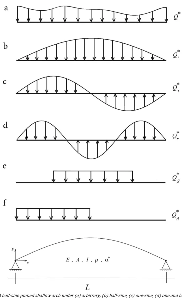
Figure 1: A half-sine pinned shallow arch under (a) arbitrary, (b) half-sine, (c) one-sine, (d) one and half-sine, (e) symmetric and (f) asymmetric loadings
deflec-tions are neglected (Chen and Yang, 2007a); and (4) The range of displacements and curvatures of the arch is small in comparison with the length of the span (0ymax/L1 / 10 1 / 50) (Xu et al., 2002). Given the above assumptions, the equation of motion can be written as follows (Plaut and Johnson, 1981; Chen and Yang, 2007b; Chen et al., 2009):
* *
,tt ( 0 ,)xxxx ,xx
Ay EI y y P y Q
(1)
where, y0 is the initial shape of the arch, the subscripts “,t” and “,
x
” show the partial differentiation with respect to the time and the longitudinal position of arch, respectively. The value of the axial force (p*) is* * 2 2
0 0 , 0,
1
( ( ) )
2
L
x x
P EA T y y dx
L
(2)Here, T0 denotes environmental temperature changes.
Since the supports are fixed at the ends, the displacement of the arch in the direction
x
is neglected. In addi-tion, the temperature change can cause the axial force in the structure, which is denoted by the term *0
EA T . Eqs. (1) and (2) could be rewritten in a dimensionless form:
, ( 0 ,) ,
u u u pu Q (3)
2 2
0 , 0,
0
1
( )
2
p T u u d
(4)where,
2 3 2
*
0 0 2 3 2 2
1
( , )u u ( , ),y y x, r Et, Q L Q*, L
r L L EIr r
(5)
Here,
r
represents the radius of gyration of the cross section calculated by r I /A. The boundary con-ditions for Eq. (3) is as follows:0 , 0, 0 , 0,
(0) (0) 0, (0) (0) 0, ( ) ( ) 0, ( ) ( ) 0
u u u u u u u u (6)
By considering the boundary conditions, the initial and deformed shapes of the arch can be rewritten in the Fourier series form:
0( ) sin
u h (7)
1
( , ) n( )sin
n
u n
(8)In Eq. (7), h is the initial dimensionless rise of the arch. The external load Q based on Fourier series can be written as
1
sin
n n
Q Q n
(9)0
2 sin , 1,2,...
n
Q Q n d n
(10)By substituting Eqs. (7)-(9) into (3), a set of equations will be obtained:
4 2 , 1,2,...
n n n pn n qn n
Here, q1 Q1h, qn Qnfor n2,3,... and pis as follows:
2 2 2
0
1
4 4
k k
k h
p T
(12)At equilibrium state, n for n 1,2,... is equal to zero. Therefore, the Eq. (11) is written as:
4 2 0 , 1,2,...
n n n n
R n pn q n (13)
where, Rnis the unbalanced force. The set of equations in (13) denotes the equilibrium state dependent on the
external load Q.
3 THE CRITICAL POINTS
In this section, the critical load of the shallow arch is addressed. If the external load is a function of an inde-pendent parameter (Q Q( )) , the solution of Eq. (13) results in a relationship between the displacement
u
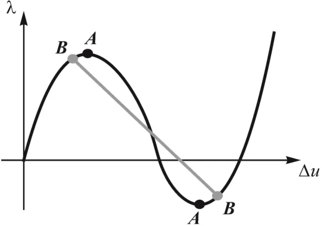
and the load factor . In the other words, the equilibrium states in the space of ( , )u represent a number of curves that are called equilibrium paths. An example of equilibrium paths is shown in Figure 2. Each point on the curves represents the position of an equilibrium state relative to the load factor.
Figure 2: Primary (black) and bifurcation (gray) equilibrium paths
One way to obtain critical points is equating the determinant of tangent stiffness matrix to zero. The (modal) tangent stiffness matrix is calculated by the derivation of the unbalanced force. This can be done by substituting the magnitude of p from Eq. (12) into Eq. (13) and taking derivatives with respect to m:
2 2
2( 2 ) , , 1,2,...
2
n
nm n m nm
m
R n m
K n n p n m
(14)
Here, nm is the Kronecker delta. By equating the determinant of Knmto zero, the critical condition
illustrat-ing limit and bifurcation points is obtained: 4
1
0 2
nm n m nm
r
r
K
(15)2 2 2 2
( )
, , 1,2,... / 2
nm nm
n n p
n m n m
(16)
The magnitude of the determinant n m nm in Eq. (15) can be calculated by the following procedure:
2 2
2
1 11 1 2 11 1
2 2
2 1 2 22 22 2
1
1 1
1 1
n m nm q
q
(17)By using algebraic operations, Eq. (17) becomes the determinant of an upper triangle matrix:
2
211 1 2 1 2 22 2 1 2 33 3
1 1 1
0 0
0 0
n
n nn
n m nm q
q
(18)Consequently, Eq. (15) is rewritten as
4 2
1 1 1
1 0
2
n
nm kk
r k n nn
r
K
(19)or
2
1 1 1
0
kk n kk
k n k
k n
(20)4 RESULTS FOR LOADING PATTERNS
In this section, the behavior of shallow arch under a number of distributed loads are separately investigated. The patterns of loadings, respectively, are half-sine Q1 sin (Figure 1(b)), one-sine Q2 sin2 (Figure 1(c)), one and half-sine Q3 sin3 (Figure 1(d)), k-sine Qk sink, symmetric step function QS (Figure
1(e)) and asymmetric step function QA (Figure 1(f)). In this way, a new formulation is proposed to achieve the
4.1 Half-sine loading
By considering the type of loading shown in Figure 1(b), the values of qn for n 1,2,... are equal to
1 0, 2,3,... n q h q n (21)
For qn 0, two types of structural responses are obtained. In the former type which is corresponding to the initial equilibrium path, the parameters n are equal to zero for n 2,3,..., while there is a non-zero n (for
instance, j) in the latter type (bifurcation path). The parameters n for the initial equilibrium path is obtained
from Eqs. (13) and (21):
1 1
0, 2, 3,...
n h p n (22)
By substituting n into Eq. (12), the value of p is calculated:
2 2
0 2
( )
4 4(1 )
h h p T p (23)
From this equation, is as follows:
2
2 0
2 2 2 2
2(1 )
2(1 ) 4(1 ) (1 ) (1 )
T
h h p
p
p p p p
(24)
By substituting (22) into Eq. (8), the displacement field of the shallow arch is obtained:
0( ) 1 sinh
u u u h
p
(25)
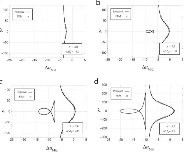
This equation is compatible with the results previously presented in the literature for a pin-ended shallow arch under a half-sine distributed loading (Plaut and Johnson, 1981). Eqs. (24) and (25) reveals the equilibrium path in the space ( , ) u for the different values of p. For example, the displacement in the middle of the span ( / 2) is equal to
( / 2) 1
Mid
h
u u h
p
(26)
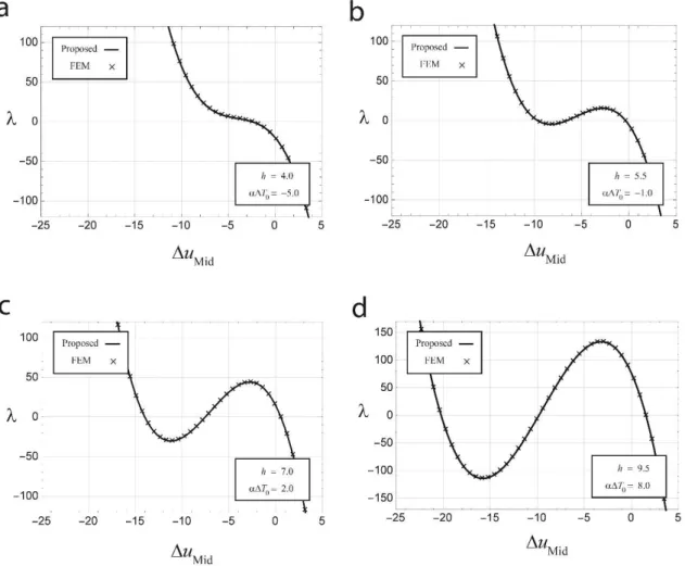
Figure 3: Initial equilibrium paths for four different values of h and T0
The comparison between the formation of curves and the result of finite element method displays the per-formance of the proposed strategy. It is noteworthy that the non-linear FEM procedure obtains a number of dis-crete equilibrium points, while a continuous equilibrium curve is given by the suggested method.
As it is mentioned previously, there is a non-zero term in bifurcation paths (j 0). From Eq. (13), the val-ue pis obtained (p j2), and by considering Eq. (12), the magnitude of
j
is calculated: 2
2 2
0 2 2
( )
2
,
4 4(1 ) 2, 3,
j
h h
T j
j j j
(27)
Similar to the initial equilibrium path, the displacement field relative to the jth bifurcation path is obtained by substituting the coefficients n into Eq. (8):
( 2 )sin sin , 2, 3,...1
j j
h
u h j j
j
(28)
This equation shows a linear relationship between and u. By considering / 2, the displacement of the midpoint in the jth bifurcation path is computed:
2
( ) sin , 2, 3,...
2 1
j Mid j
h j
u h j
j
(29)
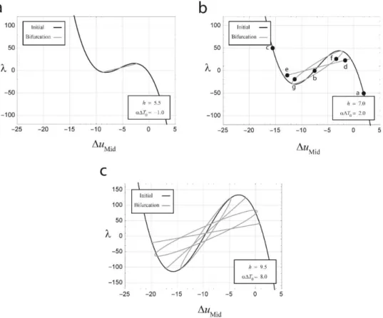
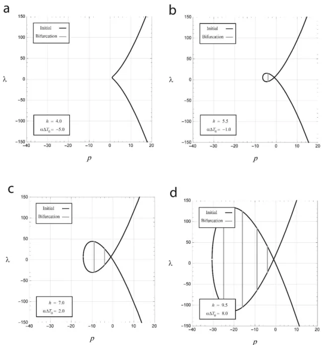
Figure 4: Initial and bifurcation paths for different values of h and T0
As it can be seen, for greater values of h and T0, the number of bifurcation paths increases. This issue
will be discussed later.
To investigate the structural behavior, a number of static states are displayed in Figure 5. These states are re-lated to points a-g specified in Figure 4(b). In this Figure, the points a-c and d-g are, respectively, corresponding to the initial and bifurcation paths.
A particular case which can be of interest is the relationship between the external load parameter and the ax-ial force along the equilibrium path. Figure 6 draws this relationship by considering Eq. (23). In this figure, four cases corresponding to the values of h and T0 given in Figure 3(a)-(d) are shown.
Figure 6: Relationship between load parameter and axial force for four different values of h and T0
The solid black and gray curves are relative to the initial and bifurcated paths, respectively. Note that, nega-tive values for the axial force p represent that the shallow arch is in compression. As it is seen, the arch is always in tension for the case (a). By increasing the parameters h and T0, the magnitude of p becomes negative in some parts of initial equilibrium paths. All bifurcation paths happen when the arch is in compression.
In order to obtain limit points, Eq. (19) can be rewritten in a simpler form: 2
1
1 n 0
n nn
By substituting the obtained values n from Eq. (22) into Eq. (30), the critical load is calculated:
2 3
( )
1 0
2(1 )
cr
h p
(31)
In this equation, cr represents the critical load. Eqs. (23) and (31) display the locus of limit points in the
space (cr,T h0, ).
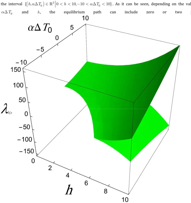
Figure 7 shows the relationship between the magnitude of critical load and the values of h and T0 for
the interval
20 0
{ ,h T R 0 h 10, 10 T 10}. As it can be seen, depending on the values of
0
T
and h, the equilibrium path can include zero or two points.
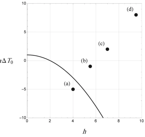
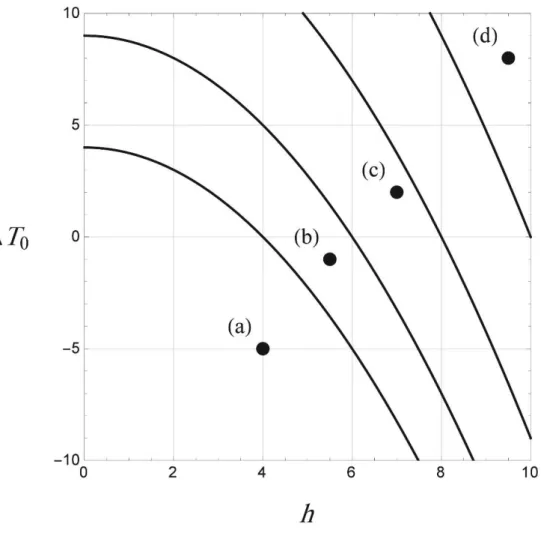
The projection of the surfaces displayed in Figure 7 on the plane of
h,T0
draws a boundary which isidentifying the number of limit points on the equilibrium path. Figure 8 illustrates the mentioned boundary and the locus of states (a)-(d) in Figure 3. As a result, the initial equilibrium paths corresponding to the upper side of the boundary (e.g. states (b)-(d)) include two limit points, while there is no limit point for the state (a). This issue would also be realized by the investigation of critical surfaces passing over the supposed h and T0 in Figure 7.
Figure 8: The boundary identifying the number of limit points in the space of
h,T0
It can be proven that the magnitude of the axial force on the boundary (BL) is constant and equal to 1. By
substituting the critical condition (31) into Eq. (23) and considering p 1, a relationship between the parame-ters h and T0 is obtained for the boundary BL:
2 20 0
, R 1
4
L
h B h T T
(32)
As previously mentioned, the bifurcation points have the following characteristics:
2
0, 2, 3,... , , 2, 3,...
n n n j
p j j
Since bifurcation points are located on both initial and bifurcation paths, these points include all properties of both paths (especially, the condition j 0). By considering Eq. (27), a relationship between h, T0 and
cr
is obtained:
2 2
2
0 2
2
( )
0, 2, 3,
4 4 1
cr j
h h
c T j j
j
(34)
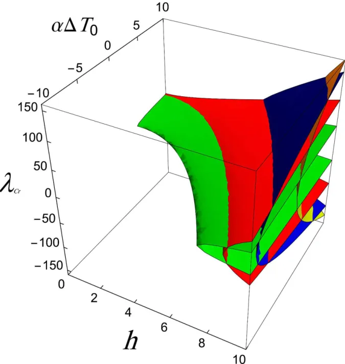
The equation cj 0 provides surfaces in the space (cr,T h0, ). These surfaces describe the value of criti-cal loads cr corresponding to bifurcation points on the equilibrium path. According to the values of h and
0
T
, the number of bifurcation points can be zero, two, four, six and eight. In Figure 9, the green, red, blue and
yellow surfaces represent the magnitude of critical points corresponding to the first, second, third and fourth bifurcation paths, respectively.
In a similar way, the boundaries which are identifying the number of bifurcation points on the equilibrium path (BB), can be derived by projecting the surfaces on the plane of h and T0. For this purpose, the con-straint cj cr 0 should be satisfied. This constraint concludes cr h. Consequently, the following
formu-lation for the set of boundaries BB is obtained from (34):
2 2 20 0
, R , 2, 3,
4
B j
h
B h T T j j
(35)
Figure 10 shows the boundaries BB j for different values of j.
Figure 10: The boundaries identifying the number of bifurcation points in the space of
h,T0
It is noteworthy that, all initial equilibrium paths corresponding to the states between two specific curves in-clude the same number of bifurcation points.
4.2 One-sine loading
2
1
0 , 3,4,....
n
q h
q
q n
(36)
If the procedure, which is previously described in the Subsection 4.1, is applied, the values of n and p will
be calculated:
1
2
1
16 4
0, 3,4,...
n
h p
p
n
(37)
2 2 2
0 4 2 2
4 1 16 4
h h
p T
p p
(38)
Additionally, the dimensionless displacement field for the initial equilibrium path is obtained from Eq. (8):
Δ 2 cos sin
1 16 4
hp u
p p
(39)
Consequently, the displacement of the midpoint is as follows:
1
Mid
u hp
p
(40)
Figure 11 displays the equilibrium paths for four different values of h and T0 . The comparison between the results given by the proposed method and the non-linear FEM shows the accuracy of the suggested technique. As it can be seen, for large values of h and T0, a secondary equilibrium path is appeared (Figure 11(b)-(d)).
Figure 11: Initial and secondary equilibrium paths for four different values of h and T0
Similar to the Subsection 4.1., j can be obtained:
2 2 2
2
0 2 2
2 2
2
,
4 4 1 16 4 3,4,
j
h h
T j j
j j j
(41)
Eqs. (42) and (43), respectively, show the displacement field and displacement of the midpoint for the jth bifurcation state:
Δ 2 2 cos 2 sin sin , 3, 4
1 16 4 ,
j j
h
u h j j
j j
(42)
2
2 sin 2 ,
1 3, 4,
j Mid j
hj j
j j
u
(43)
Figure 12: Initial, secondary and bifurcation paths for different values of h and T0
In addition, to have a better analogy, the relationship between the load parameter and the axial force is given in Figure 13.
Figure 14 shows the equilibrium states relative to the points a-g in Figure 12(a).
Figure 14: Equilibrium states corresponding to the points a-g shown in Figure 12(a)
In order to obtain the locus of limit points, the values of n given by Eq. (37) are substituted into Eq. (30):
2 2
3 3
2
1 0
2 1 16 4
cr
h
p p
(44)
Eqs. (38) and (44) reveal the location of limit points as a set of surfaces in the space of (cr,T h0, ). For the
interval
20 0
Figure 15: The locus of limit points in the space of
cr, T h0,
On the other hand, the equation (45) should be satisfied for the bifurcation points on the jth bifurcation path:
2
0, 3, 4,... , , 3, 4,...
n n n j
p j j
(45)
By considering p j2 in Eq. (38), an explicit relationship between h, 0
T
and cr is achieved:
2
2 2
2
0 2 2
2 2 0, 3, 4,
4 4 1 16 4
cr j
h h
c T j j
j j
Figure 16 shows surfaces cj 0 for
20 0
{ ,h T R 0 h 10, 10 T 10}. The green, red and blue surfaces represent the magnitude of bifurcation points corresponding to the first, second and third bifurcat-ed paths, respectively.
Figure 16: The locus of bifurcation points in the space of
cr, T h0,
4.3 One and half-sine loading
If the loading pattern is assumed to be Q3 sin3 (Figure 1(d)), the values of qn and subsequently the
2 1
3
0
, 4, 5,.... 0
n
q h
q q
q n
(47)
2 1
3
1
9 9
4,5,... 0
0,
n
h p
p n
(48)
Furthermore, the calculated parameters p, u and uMid are respectively given by Eqs. (49)-(51):
2 2 2
0 4 2 2
4 1 36 9
h h
p T
p p
(49)
Δ sin sin 3
1 9 9
hp u
p p
(50)
1 9 9
Mid
hp p u
p
(51)
Figure 17 shows the equilibrium paths for four different values of h and T0. The solid curves and the signs , respectively, represent the obtained responses of the proposed technique and the finite element method.
In a similar way, the displacement field and displacement of midpoint for the jth bifurcation path can be cal-culated:
Δ 22sin 2 sin 3 sin , 2,4,5,...
1 9 9
j j
hj
u j j
j j
(52)
2
2 2 sin 2 , 2,4,5,...
1 9 9
j Mid hj j j j
u
j j
(53)
By considering Eq. (12), j is computed:
2 2 2
2
0 2 2
2 2
2
, 2, 4, 5,...
4 4 1 36 9
j
h h
T j j
j j j
(54)
In Figure 18, the bifurcation paths are denoted by gray curves.
Figure 18: Initial, secondary and bifurcation paths for different values of h and T0
Figure 19: Equilibrium states corresponding to the points a-f shown in Figure 18(b)
Figure 18 shows that the initial equilibrium path does not include any critical point, and all critical points (limit and bifurcation) are located on the second equilibrium path. By substituting the values of n into Eq. (30),
the critical load is calculated:
2 2
3 3
1 0
2 1 18 9
cr
h
p p
(55)
The locus of limit points in the interval
20 0
{ ,h T R 0 h 10, 10 T 10} is presented in Fig-ure 20:
On the other hand, the bifurcation points should satisfy the following conditions:
2
0, 2, 4, 5,..., , 2, 4,5,...
n n n j
p j j
(56)
By substituting the value p from Eq. (56) into Eq. (49), the location of bifurcation points in the space of
0
, )
(cr T h, is obtained:
2
2 2
2
0 2 2
2 0, 2, 4, 5,...
4 4 1 4 9
cr j
h h
c T j j
j j
(57)
The locus of bifurcation points for the interval
20 0
{ ,h T R 0 h 10, 10 T 10} is shown in Figure 21. The green, red and blue surfaces represent the magnitude of bifurcation points corresponding to the first, second and third bifurcated paths, respectively.
4.4 k-sine loading
In this subsection, the effect of general sinusoidal loading pattern (Qk sink) on the structural behavior of the shallow arch is investigated. The parameter k describes the formation of the external loading. Based on
this supposition, the magnitude of qn for n 1,2,3, can be calculated for different values of k:
1 , 1
1 :
0, 2,3,
n
q h n
k q n (58)
1 , 1
2,3,... : n 0, 2, 3,... ,
k
q h n
k q n n k
q (59)
By considering Eqs. (13), (58) and (59), the coefficients n are obtained in a generalized form:
1
(I): 1
0 , 2, 3,
n h P n (60) 1 2 1
(II): n 0, 2, 3,... ,
j
h p
n n j
from p j (61) 1 2 2 1
(III): 0, 2, 3,... ,
( )
n k
h p
n n k
k k p (62) 1 2 2 2 1
0, 2, 3,... , ,
(IV): ( ) n k j h p
n n k n j
k k p from p j (63)
The States I and II are corresponding to k 1, while the others are relative to the condition k 1. Addi-tionally, the States I and III can describe the initial equilibrium path. For this purpose, the magnitude of axial force is calculated by substituting Eqs. (60) and (62) into (12):
22
0 2
(I):
4 4(1 )
h h p T p (64)
2 2 2
0 2 2
2 2
(III):
4 4(1 ) 4
h h
p T
p k k p
(65)
Δ (I): sin 1 h u h p
(66)
Δ 2
2 2
(III): sin sin
1 h
u h k
p k k p
(67)
On the other hand, the States II and IV, are corresponding to the bifurcation equilibrium path. Similarly, the displacement field for the j th bifurcation path can be derived:
Δ 2
(II): sin sin
1
j j
h
u h j
j
(68)
Δ 2 2 2 2
(IV): sin sin sin
1
j j
h
u h k j
j k k j
(69)
The displacement of the midpoint is obtained when / 2 for the four mentioned states. The parameter
j
for the States II and IV are calculated by substituting Eqs. (61) and (63) into (12) and considering p j2:
2 2 2 0 2 2 2 (II):4 4 1
j h h T j j j (70)
2 2 2
2
0 2 2
2 2 2 2
2 (IV):
4 4 1 4
j
h h
T j
j j k k j
(71)
In order to find limit points on the initial equilibrium path, Eq. (30) is applied:
2
3
(I): 1 0
2 1 cr h p (72)
2 2 23 2 2 2 2
(III): 1 0
2 1 2
cr
k h
p k p k k p
(73)
Furthermore, the condition (74) should be satisfied for the jth bifurcation point:
2
0, 2, 3,..., ,
, 2, 3,...,
n n n k n j
p j j j k
(74)
By substituting Eq. (74) into Eqs. (64) and (65), the locus of bifurcation points is computed:
2 2 2 0 2 2(I),(II): 0
4 4 1
cr j
h h
c T j
j (75)
2 2 2 20 2 2
2 2 2 2
(III),(IV): 0
4 4 1 4
cr j
h h
c T j
j k k j
(76)
4.5 Symmetric step loading
A type of symmetric step load is shown in Figure 1(e). This loading pattern can be defined in the following form:
0 0.250 0.250.75 and 0.75Q
(77)
By using the Fourier series, the values of qn for n 1,2,... are obtained:
1
2 2
4 sin sin , 2, 3,...
2 4 n q h n n q n n (78)
Note that for even values of
n
, the magnitude of qn is equal to zero. If the procedure, which is previouslyde-scribed, is applied, the values of n and p will be calculated:
2 2
3 2
1
sin sin
2 4 , 2, 3 .
1 , .. 4 n n n n n n p p h (79)
2 2 20 2 2 ,1
2
4 4 1 1 S
h
h h
p T p
p p
(80)
where, the function S i,
p is defined in Appendix. The displacement field u
and the displacement of the midpoint u
/ 2
for the initial equilibrium path are obtained from Eq. (8):
2
1 3
sin 2 1 2 1
4
sin 2 1
1 2 sin 2 4 1 n 2 s 1 i i i i hp i
p i i
u p
(81)
,2 1 Mid S hp p pu
(82)
Figure 22: Initial equilibrium paths for four different values of h and T0
In the case of bifurcation path, there is a non-zero n for even values of
n
(e.g., 2j 0). Subsequently, theaxial force is equal to p 4j2 based on Eq. (13). By considering Eq. (12), 2j
is achieved:
2 2
2 2 2
2 0 2 2 ,1
2 2
2 1
4 4 , 1
4 4 1 4 1 4 ,2,
j S
h
h h
T j j j
j j j
(83)
Eqs. (84) and (85), respectively, show the displacement field and displacement of the midpoint for the jth bifurcation state:
Δ 3 2 2 2 2 1 2 4 sin 2 1 42 1 2 1
4
sin 2 1 , 1
2 1 2
sin
sin sin
2 4 ,2,
1 4 j j i h j j u j i i i j
i i j
(84)
2 2 ,2 2 44 , 1
1 4 S ,2,
j Mid
j h
j j
j
u
(85)
Figure 23: Initial and bifurcation paths for different values of h and T0
By substituting the values of n into Eq. (30), the critical load is calculated:
2
2 , 3
3 3
2 2
1 0
2 1 1 cr S cr
h h
p
p p
(86)
The locus of limit points in the interval
20 0
{ ,h T R 0 h 10, 10 T 10} is presented in Fig-ure 24. In this figFig-ure, each surface demonstrates a couple of limit points corresponding to the specific h and
0
T .
On the other hand, by substituting the value p 4j2 into Eq. (80), the location of bifurcation points in the space of (cr,T h0, ) is obtained:
2 2
2 2 2
0 2 2 ,1
2 2
2
4 4 0, 1,2,...
4 4 1 4 1 4
j cr S cr
h
h h
c T j j j
j j
(87)
The locus of bifurcation points for the interval
20 0
{ ,h T R 0 h 10, 10 T 10} is shown in Figure 25. The green and red surfaces represent the magnitude of bifurcation points corresponding to the first and second bifurcated paths, respectively.
4.6 Asymmetric step loading
An asymmetric step load is shown in Figure 1(f). This loading pattern is defined as
0 0.50 0.5Q
(88)
The values of qn for n 1,2,... are achieved by using the Fourier series:
1
2
2
4
sin , 2, 3,...
4 n q h n q n n (89)
It is noteworthy that the magnitude of qn is equal to zero when n 4j (for j 1,2,). Similar to
Subsec-tion 4.5, the values of n and p can be calculated:
2 1 3 2 2 sin 4, 2, 3,..
1 4 . n n n n h p p n (90)
2 2 20 4 2 2 ,1
4 1 1 A
h h h
p T p
p p
(91)
where, the function A i,
p is defined in Appendix. Subsequently, the values of u
and uMid for the initialequilibrium path are
1 1 3 2 3 2sin 2 1
1 2 1 2 1
sin 4 2 2
sin
4
4 2 4 2
i
i
u hp i
p i i
i i i p p
(92)
,2 1 Mid A hp p pu
(93)
Figure 26: Initial equilibrium paths for four different values of h and T0
As it is observed, the procedure of FEM becomes divergent in Figure 26(d).
In the case of asymmetric loading, there can be a non-zero 4j for the jth bifurcation path. Consequently,
the axial force p equals 16j2 according to Eq. (13). By considering Eq. (12), 4j
will be obtained:
2 2
4 0 2
2
1 2
2 2 2
,1 2
2
1
2 4 4 1 16
16 16 , 1
1 16 ,2, j A h h T j j
h j j j
j (94)
Accordingly, the displacement field and displacement of the midpoint for the jth bifurcation state are as fol-lows:
2
2 3 2 2
3
4 2 2
1
1
16
sin 2 1
1 16 2 1 2 1 16
sin
2 si
4 sin 4
n
2 , 1
4 2 4 , , 4 16 2 2 i j i j h i
j i i j
2
2 ,2
2
16
16 1 16
Mid A
u j h j
j
(96)
In the asymmetric step loading, there is only one bifurcation path which can be seen in the case of h 9.5 and T0 8.0 (the gray solid curve in Figure 27).
Figure 27: Initial and bifurcation paths for h9.5 and T0 8.0
Similar to the previous subsection, the locus of limit points can be determined. In this way, the critical con-straint (30) is rewritten in the following form by considering Eq. (90):
2
2 ,3
3 3
2
1 0
2 1 1 cr A cr
h h
p
p p
(97)
The locus of limit points in the interval
20 0
Figure 28: The locus of limit points in the space of
cr, T h0,
In order to find the location of bifurcation points in the space of (cr,T h0, ), Eq. (91) with the constraint 2
16
p j is applied:
2 2
0 2
2
2 2 2
,1 2
2
4 4 1 16
16 16 0, 1,2,...
1 16
j
cr A cr
h h
c T
j h
j j j
j
(98)
The locus of bifurcation points for the interval
20 0
Figure 29: The locus of bifurcation points in the space of
cr, T h0,
5 CONCLUSIONS
The stability behavior of shallow arches is always being of the researchers’ interest. In this paper, an analyti-cal method to find the exact solution of a half-sinusoidal elastic shallow arch in the thermal environment under sinusoidal and step loads is proposed. For this purpose, the structural displacement is rewritten in a form of Fou-rier series, and subsequently, both initial and bifurcated equilibrium paths are obtained by substituting the trans-formed displacements into the governing equations of the arch. In addition, the critical points (such as limit and bifurcation points) are calculated by equating the determinant of stiffness matrix to zero. Furthermore, a new generalized formulation for various types of sinusoidal loadings is proposed.
com-prehensively. Moreover, finding the critical points without tracing the equilibrium path is the superiority of the suggested technique.
Acknowledgements
The authors gratefully acknowledge the helpful suggestions received from the anonymous reviewers. The quality of this article has benefited substantially from their comments.
References
Bateni, M. and Eslami, M.R. (2015). Non-linear in-plane stability analysis of FG circular shallow arches under uni-form radial pressure, Thin-Walled Structures 94: 302-313.
Bradford, M.A., Pi, Y.-L., Yang, G. and Fan, X.-C. (2015). Effects of approximations on non-linear in-plane elastic buckling and postbuckling analyses of shallow parabolic arches, Engineering Structures 101: 58-67.
Cai, J., Xu, Y., Feng, J. and Zhang, J. (2012). In-plane elastic buckling of shallow parabolic arches under an external load and temperature changes, Journal of structural engineering 138(11): 1300-1309.
Chandra, Y., Stanciulescu, I., Eason, T. and Spottswood, M. (2012). Numerical pathologies in snap-through simula-tions, Engineering Structures 34: 495-504.
Chen, J.S. and Hung, S.Y. (2012). Exact snapping loads of a buckled beam under a midpoint force, Applied Mathe-matical Modelling 36: 1776-1782.
Chen, J.S. and Li, Y.T. (2006). Effects of elastic foundation on the snap-through buckling of a shallow arch under a moving point load, International Journal of Solids and Structures 43(14): 4220-4237.
Chen, J.S. and Liao, C.Y. (2005). Experiment and analysis on the free dynamics of a shallow arch after an impact load at the end, ASME Journal of Applied Mechanics 72(1): 54-61.
Chen, J.S. and Lin, J.S. (2005). Exact critical loads for a pinned half-sine arch under end couples, ASME Journal of Applied Mechanics 72(1): 147-148.
Chen, J.S. and Ro, W.C. (2009). Dynamic response of a shallow arch under end moments, Journal of Sound and Vibration 326(1): 321-331.
Chen, J.S., Ro, W.C. and Lin, J.S. (2009). Exact static and dynamic critical loads of a sinusoidal arch under a point force at the midpoint, International Journal of Non-Linear Mechanics 44(1): 66-70.
Chen, J.S. and Yang, C.H. (2007a). Experiment and theory on the nonlinear vibration of a shallow arch under har-monic excitation at the end, ASME Journal of Applied Mechanics 74(1): 1061-1070.
Chen, J.S. and Yang, M.R. (2007b). Vibration and stability of a shallow arch under a moving mass-dashpot-spring system, ASME Journal of Vibration and Acoustics 129: 66-72.
Crisfield, M.A. (1991). Non-linear Finite Element Analysis of Solids and Structures, Volume 1: Essentials, J. Wiley and Sons, Chichester.
Crisfield, M.A. (1997). Non-linear Finite Element Analysis of Solids and Structures, Volume 2: Advanced Topics, J. Wiley and Sons, Chichester.
Han, Q., Cheng, Y., Lu, Y., Li, T. and Lu, P. (2016). Nonlinear buckling analysis of shallow arches with elastic hori-zontal supports, Thin-Walled Structures 109: 88-102.
Hung, S.Y. and Chen, J.S. (2012). Snapping of a buckled beam on elastic foundation under a midpoint force, Euro-pean Journal of Mechanics-A/Solids 31(1): 90-100.
Khalil, H.K. (2002). Nonlinear Systems, Prentice Hall.
Kiani, Y. and Eslami, M.R. (2013). Thermomechanical buckling of temperature-dependent FGM beams, Latin American Journal of Solids and Structures 10: 223-246.
Matsunaga, H. (1996). In-plane vibration and stability of shallow circular arches subjected to axial forces, Interna-tional Journal of Solids and Structures 33(4): 469-482.
Moghaddasie, B. and Stanciulescu, I. (2013a). Direct calculation of critical points in parameter sensitive systems, Computers & Structures 117: 34-47.
Moghaddasie, B. and Stanciulescu, I. (2013b). Equilibria and stability boundaries of shallow arches under static loading in a thermal environment, International Journal of Non-Linear Mechanics 51: 132-144.
Moon, J., Yoon, K.Y., Lee, T.H. and Lee, H.E. (2007). In-plane elastic buckling of pin-ended shallow parabolic arches, Engineering Structures 29(10): 2611-2617.
Pi, Y.-L. and Bradford, M.A. (2012). Non-linear buckling and postbuckling analysis of arches with unequal rota-tional end restraints under a central concentrated load, Internarota-tional Journal of Solids and Structures 49(26): 3762-3773.
Pi, Y.-L. and Bradford, M.A. (2013). Nonlinear elastic analysis and buckling of pinned–fixed arches, International Journal of Mechanical Sciences 68: 212-223.
Pi, Y.-L., Bradford, M.A. and Qu, W. (2010). Energy approach for dynamic buckling of shallow fixed arches under step loading with infinite duration, Structural Engineering and Mechanics 35(5): 555-570.
Pi, Y.-L., Bradford, M.A. and Tin-Loi, F. (2007). Nonlinear analysis and buckling of elastically supported circular shallow arches, International Journal of Solids and Structures 44(7-8): 2401-2425.
Pi, Y.-L., Bradford, M.A. and Tin-Loi, F. (2008). Non-linear in-plane buckling of rotationally restrained shallow arches under a central concentrated load, International Journal of Non-Linear Mechanics 43(1): 1-17.
Pi, Y.-L., Bradford, M.A. and Uy, B. (2002). In-plane stability of arches, International Journal of Solids and Struc-tures 39(1): 105-125.
Pippard, A.B. (1990). The elastic arch and its modes of instability, European Journal of Physics 11: 359-365.
Plaut, R.H. (2009). Snap-through of shallow elastic arches under end moments, ASME Journal of Applied Mechan-ics 76: 014504.
Plaut, R.H. and Johnson, E.R. (1981). The effects of initial thrust and elastic foundation on the vibration frequen-cies of a shallow arch, Journal of Sound and Vibration 78(4): 565-571.
Reddy, B.D. and Volpi, M.B. (1992). Mixed finite element methods for the circular arch problem, Computer meth-ods in applied mechanics and engineering 97(1): 125-145.
Rezaiee-Pajand, M. and Moghaddasie, B. (2014). Stability boundaries of two-parameter non-linear elastic struc-tures, International Journal of Solids and Structures 51(5): 1089-1102.
Rezaiee-Pajand, M. and Rajabzadeh-Safaei, N. (2016). An explicit stiffness matrix for parabolic beam element, Latin American Journal of Solids and Structures 13: 1782-1801.
Saffari, H., Mirzai, N.M. and Mansouri, I. (2012). An accelerated incremental algorithm to trace the nonlinear equi-librium path of structures, Latin American Journal of Solids and Structures 9: 425-442.
Stanciulescu, I., Mitchell, T., Chandra, Y., Eason, T. and Spottswood, M. (2012). A lower bound on snap-through instability of curved beams under thermomechanical loads, International Journal of Non-Linear Mechanics 47(5): 561-575.
Thompson, J.M.T. and Hunt, G.W. (1973). A General Theory of Elastic Stability, J. Wiley.
Tsiatas, G.C. and Babouskos, N.G. (2017). Linear and geometrically nonlinear analysis of non-uniform shallow arches under a central concentrated force, International Journal of Non-Linear Mechanics 92: 92-101.
Virgin, L.N., Wiebe, R., Spottswood, S.M. and Eason, T.G. (2014). Sensitivity in the structural behavior of shallow arches, International Journal of Non-Linear Mechanics 58: 212-221.
Xenidis, H., Morfidis, K. and Papadopoulos, P.G. (2013). Nonlinear analysis of thin shallow arches subject to snap-through using truss models, Structural Engineering and Mechanics 45(4): 521-542.
Xu, J.X., Huang, H., Zhang, P.Z. and Zhou, J.Q. (2002). Dynamic stability of shallow arch with elastic supports— application in the dynamic stability analysis of inner winding of transformer during short circuit, International Journal of Non-Linear Mechanics 37(4): 909-920.
Zhou, Y., Chang, W. and Stanciulescu, I. (2015a). Non-linear stability and remote unconnected equilibria of shal-low arches with asymmetric geometric imperfections, International Journal of Non-Linear Mechanics 77: 1-11.
APPENDIX
Here, the functions S i,
p and A i,
p are defined and their magnitudes are given for some values of i:
,1 2 4 2 2 2 23 2 3 7/2
2
1 2
sech 5 tanh
1
2
2 1 2 1
2 48 8 4
p p
S
i
p
i
p p p
i p p
(A.1)
2 4 22 2 2
1
,2 3 2
1
2
1 1 1
cot 3 csc 1 tan 3
1 3 8 4 8
32 4 2 2 2 4
4 sin
2 1 2 1
2
i S
i
p p p
p p p i p p p i p
(A.2)
, 3 3
4
2 2
2 2 2 2
2
4 3 4 9/2 7
2 1
/2 2
11 sech 35 tanh sech tanh
3
2 24 16 8 16
4
2 1 2 1
p S i p p p p p i i
p p p p
p
(A.3)
,1 2 2
4 2
2 2
2 4 2
4 2
3 2 3 3 7/2 7/2
4 2
1 2 1 2
sech sech 5 tanh 5 tanh
1 5
2 384 16 1
1 4
2 1 2 1 4 2 4 2
6 4 8
p p p p
A
i i
p p p p p
p
i i p i i p
p
(A.4)
,2 3 2
1
2
2
2 2
2 1
2 1 2 1
sech 1 16 2 2 i A i p p i i p p p p
(A.5)
2 22 4 2
4 4
, 3 3 3
4 2 4 2
1
3 4 4 9/2
2 2
4 4 2 2 2
7/2 9/2 /
2 7 1 2 2 2
11 sech 11 sech 35 tanh
3 5
2 192 32 32 8
sech tanh 35 ta sech tanh
8
2 1 2 1 4 2 4 2
nh
64 16 32
p p p
p p A i i p p p p
i i p i i p
p p p p p
p p p