Lat. Am. j. solids struct. vol.11 número9

(1)

Abs tract

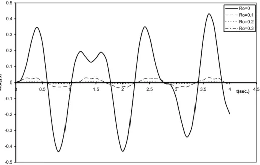
The flexural motions of elastically supported rectangular plates carrying moving masses and resting on variable Winkler elastic foundations is investigated in this work In order to solve the fourth order partial differential equation governing the problem, a technique based on separation of variables is used to reduce the governing fourth order partial differential equations with variable and singular coefficients to a sequence of second order ordinary differential equations. These equations are then solved using a modification of the Struble’s technique and method of integral transformations. Numerical results are then presented in plotted curves. The results show that response amplitudes of the plate decrease as the value of the rotatory inertia correction factor Ro

increases and for fixed value of Ro, the displacements of the

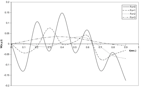
elasti-cally supported rectangular plates resting on variable elastic foun-dations decrease as the foundation modulus Fo increases. Also, for

fixed Ro and Fo, the transverse deflections of the rectangular

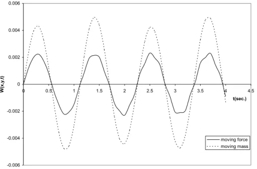
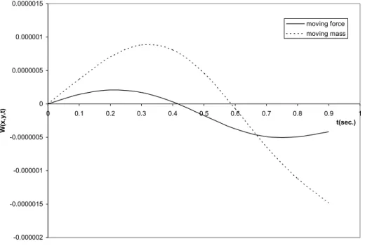
pla-tes under the actions of moving masses are higher than those when only the force effects of the moving load are considered. Therefore, the moving force solution is not a safe approximation to the mo-ving mass problem. Hence, safety is not guaranteed for a design based on the moving force solution. Furthermore, the results show that the critical speed for the moving mass problem is reached prior to that of the moving force for the elastically supported rectangular plates on Winkler elastic foundation with stiffness variation.

Key words

Winkler Foundation, Foundation Modulus, Rotatory Inertia, Re-sonance, Critical Speed, Moving Force, Moving Mass.

Flexural motions under moving concentrated masses of

elastically supported rectangular plates resting on

va-riable winkler elastic foundation

T. O. Awodola*

Department of Mathematical Sciences Federal University of Technology, Akure, Nigeria

(2)

Latin American Journal of Solids and Structures 11 (2014) 1515-1540 1 INTRODUCTION

The analyses of elastic structures, such as beams and plates, acted upon by moving loads and resting on a foundation constitute an important part of Engineering and applied Mathematics literatures. In general, such analyses are mathematically complex due to the difficulty in modeling the mechanical response of the subgrade which is governed by many factors.

When the vehicle-track interaction is completely neglected, we have the so called ‘moving for-ce’ problem which has been shown by several researchers that it is a crude approximation to the ‘moving mass’ problem where the vehicle-track interaction is considered, Muscolino and Palmeri (2007). Several researchers have considered the vehicle-track interaction in their analyses. These researchers include Stanisic et al (1974), Milornir et al (1969), Clastornic et al (1986), Sadiku and Leipholz (1981) and Gbadeyan and Oni (1995). Douglas et al (2002) solved the problem of plate strip of varying thickness and the center of shear. In their work, they considered a free-vibrating strip with classical boundary conditions, precisely, they assumed the plate strip clamped at one end and free at the other end. Pesterev et al (2001) came up with a series expansion method for calculating bending moment and shear force in the problem of vibration of a damped beam sub-ject to an arbitrary number of moving loads. This kind of solution, though could be accurate, cannot account for vital information such as the phenomenon of resonance in the dynamical sys-tem.

Recently, several other researchers have made tremendous efforts in the study of dynamics of structures under moving loads, these include Oni (2004), Oni and Omolofe (2005), Oni and Awodola (2003), Omer and Aitung (2006), Adams (1995), Savin (2001), Jia-Jang (2006). In all of these, considerations have been limited to cases of one-dimensional (beam) problems. Where two-dimensional (plate) problems have been considered, the foundation moduli are taken to be con-stants. No considerations have been given to the class of dynamical problems in which the foun-dation is the type with stiffness variation. In an attempt to solve such two-dimensional problem, all the methods used in the above works break down due to the variation of the foundation mod-el.

Generally, the dynamical problems of structures under moving load and resting on a founda-tion is complex, the complexity increases if the foundafounda-tion stiffness varies along the structure. Aside the problem of singularity brought in by the inclusion of the inertia effects of the moving load, the coefficients of the governing fourth order partial differential equation are no longer con-stant but variable. Earlier researchers into beam member on variable elastic foundation include Franklin and Scott (1979) who presented a closed-form solution to a linear variation of the foun-dation modulus using contour-integrals. In a recent development, Oni and Awodola (2005) inves-tigated the dynamic response to moving concentrated masses of uniform Rayleigh beams resting on variable Winkler elastic foundation.

(3)

Latin American Journal of Solids and Structures 11 (2014) 1515-1540 example is the elastically supported end conditions. As a problem of this kind, Wilson (1974) studied the response of a cantilever plate strip restrained elastically against rotation and subject-ed to a moving normal line load.

More recently, Oni and Awodola (2010) considered the dynamic response under a moving load of an elastically supported non-prismatic Bernoulli-Euler beam on variable elastic foundation. The technique was based on the generalized Galerkin’s method and integral transformations.

In all these previous investigations, extension of the theory to cover two-dimensional (plate) problem has not been effected, when the plate is on variable foundation. Therefore, this study concerns the response to moving concentrated masses of elastically supported rectangular plate resting on Winkler elastic foundation with stiffness variation.

2 G O V E R N IN G E Q U A T IO N

Consider a rectangular plate carrying an arbitrary number (say N) of concentrated masses Mi

moving with constant velocities ci, i = 1, 2, 3, … , N along a straight line parallel to the x – axis

( no difficulty arises by assuming that masses travel in an arbitrary path ) issuing from point y = s on the y – axis. The equation governing the dynamic transverse displacement W(x,y,t) of an elastically supported rectangular plate when it is resting on a variable Winkler foundation and traversed by several moving concentrated masses is the fourth order partial differential equation given by; Oni and Awodola (2011),

D

∇

4

W

(

x

,

y

,

t

)

+

µ

∂

2

W

(

x

,

y

,

t

)

∂

t

2

=

µ

R

0

∂

4

∂

t

2

∂

x

2

+

∂

4

∂

t

2

∂

y

2

⎡

⎣

⎢

⎤

_⎦

⎥

W

(

x

,

y

,

t

)

−

F

₀

⎡⎣

4 x

−

3 x

2

+

x

3

⎤⎦

W

(

x

,

y

,

t

)

+

[

M

_i

g

δ

(

x

−

c

_i

t

)

δ

(

y

−

s

)

i=1 N

∑

−

M

_i

∂

2

∂

t

2

+

2 c

i

∂

2

∂

t

∂

x

+

c

i 2

∂

2

∂

x

2

⎛

⎝⎜

⎞

⎠⎟

W

(

x

,

y

,

t

)

δ

(

x

−

c

i

t

)

δ

(

y

−

s

)

]

(1)

where

D

₌

Eh

2

12(1

₋

v

₎

(2)

is the bending rigidity of the plate,

∇

2_{is the two-dimensional Laplacian operator, h is the plate’s}

thickness, E is the Young’s Modulus,

v

_{is the Poisson’s ratio}

(

v

_<

1)

,

µ

is the mass per unit

area of the plate,

_R

₀ is the Rotatory inertia correction factor, F0 is the foundation‘s stiffness, g is

the acceleration due to gravity, x and y are respectively the spatial coordinates in x and y

direc-tions and t is the time coordinate. δ(.) is the Dirac – Delta function.

(4)

Latin American Journal of Solids and Structures 11 (2014) 1515-1540

W

(

x

,

y

,

t

)

₌

0 ₌

∂

W

(

x

,

y

,

t

)

∂

t

(3)

In this paper, in the first instance, we consider rectangular plate resting on a variable Winkler

elastic foundation elastically supported at edges y = 0, y = LY with simple support at edges x =

0, x = LX, the boundary conditions can be written as; Oni and Awodola (2010)

W

(0,

y

,

t

)

₌

0,

W

(

L

_X

,

y

,

t

)

₌

0

₍₄₎

∂

2

W

(

x

, 0,

t

)

∂

_y

2

−

k

1

∂

_W

(

x

, 0,

t

)

∂

_y

=

0,

∂

2

W

(

x

,

L

_Y

,

t

)

∂

_y

2

−

k

1

∂

_W

(

x

,

L

_Y

,

t

)

∂

_y

=

0

(5)

∂

2

W

(0,

y

,

t

)

∂

_x

2

=

0,

∂

2

W

(

L

X

,

y

,

t

)

∂

_x

2

=

0

(6)

∂

3

W

(

x

, 0,

t

)

∂

_y

3

+

k

2

W

(

x

, 0,

t

)

=

0,

∂

3

W

(

x

,

L

_Y

,

t

)

∂

_y

3

+

k

2

W

(

x

,

L

Y

,

t

)

=

0

(7)

and for normal modes

Ψ

ni

(0)

=

0,

Ψ

ni

(

L

X

)

=

0

(8)

∂

2

_Ψ

nj

(0)

∂

_y

2

−

k

1

∂Ψ

nj

(0)

∂

_y

=

0,

∂

2

_Ψ

nj

(

L

Y

)

∂

_y

2

−

k

1

∂Ψ

nj

(

L

Y

)

∂

_y

=

0

(9)

∂

2

_Ψ

ni

(0)

∂

x

2

=

0,

∂

2

_Ψ

ni

(

L

X

)

∂

x

2

=

0

(10)

∂

3

_Ψ

nj

(0)

∂

_y

3

+

k

2

Ψ

nj

(0)

=

0,

∂

3

_Ψ

nj

(L

Y

)

∂

_y

3

+

k

2

Ψ

nj

(L

Y

)

=

0

(11)

where k1 is the stiffness against rotation and k2 is the stiffness against translation.

Secondly, we consider an elastic rectangular plate resting on a variable Winkler elastic founda-tion and having elastic supports at all its edges, the boundary condifounda-tions are given by; Oni and Awodola (2010)

∂

2

W

(0,

y

,

t

)

∂

_x

2

−

k

1

∂

_W

(0,

y

,

t

)

∂

_x

=

0,

∂

2

W

(

L

_X

,

y

,

t

)

∂

_x

2

−

k

1

∂

_W

(

L

_X

,

y

,

t

)

(5)

∂

2

W

(

x

, 0,

t

)

∂

_y

2

−

k

1

∂

_W

₍

_x

_{, 0,}

_t

₎

∂

_y

=

0,

∂

2

W

(

x

,

L

Y

,

t

)

∂

_y

2

−

k

1

∂

_W

₍

_x

_,

_L

Y

,

t

)

∂

_y

=

0

(13)

∂

3

W

(0,

y

,

t

)

∂

_x

3

+

k

2

W

(0,

y

,

t

)

=

0,

∂

3

W

(

L

_X

,

y

,

t

)

∂

_x

3

+

k

2

W

(

L

X

,

y

,

t

)

=

0

(14)

∂

3

W

(

x

, 0,

t

)

∂

_y

3

+

k

2

W

(

x

, 0,

t

)

=

0,

∂

3

W

(

x

,

L

_Y

,

t

)

∂

_y

3

+

k

2

W

(

x

,

L

Y

,

t

)

=

0

(15)

and for normal modes

0 )

(

)

(

,

0 )

0 (

)

0 (

1 2 2 1 2 2

=

∂

Ψ

∂

−

∂

Ψ

∂

=

∂

Ψ

∂

−

∂

Ψ

∂

x

L

k

x

L

x

k

x

Y ni Y ni ni ni (16)

0 )

(

)

(

,

0 )

0 (

)

0 (

1 2 2 1 2 2

=

∂

Ψ

∂

−

∂

Ψ

∂

=

∂

Ψ

∂

−

∂

Ψ

∂

y

L

k

y

L

y

k

y

Y nj Y nj nj nj (17)

0 )

(

)

(

,

0 )

0 (

)

0 (

2 3 3 2 3 3

=

Ψ

+

∂

Ψ

∂

=

Ψ

+

∂

Ψ

∂

Y ni Y ni ni

ni

_k

_L

x

L

k

x

(18)

∂

3

_Ψ

nj

(0)

∂

_y

3

+

k

2

Ψ

nj

(0)

=

0,

∂

3

_Ψ

nj

(L

Y

)

∂

_y

3

+

k

2

Ψ

nj

(L

Y

)

=

0

(19)

where k1 and k2 are the stiffness against rotation and the stiffness against translation respectively.

3 A N A LY T IC A L A P P R O X IM A T E SO LU T IO N

The method of analysis involves expressing the Dirac – Delta function as a Fourier cosine series. Because of the variable foundation term, the elegant method of the generalized integral transform breaks down while the generalized Galerkin’s method used in one-dimensional structural problems (Beam problems) could not handle the two-dimensional structural problem (Plate problems). Thus, In order to solve equation (1), in the first instance, the deflection is written in the form; Shadnam et al (2001)

W

(x,

y,

t

)

₌

ϕ

n

(x,

y)T

n

(t

)

n=1

∞

(6)

where φn are the known eigenfunctions of the plate with the same boundary conditions. The φn

have the form of

∇

4

ϕ

n

−

ω

n 4

ϕ

n

=

0

(21)

where

ω

_n4

₌

Ω

n

2

_µ

D

(22)

Ωn, n = 1, 2, 3, … , are the natural frequencies of the dynamical system and Tn(t) are amplitude

functions which have to be calculated.

At this juncture, the right hand side of equation (1) is written in the form of a series and we have

R0

∂4

∂t2∂x2 + ∂

4

∂t2∂y2

⎡

⎣⎢

⎤

⎦⎥

W(x,y,t)− F0

µ

4x−3x2+x3

[

]

W(x,y,t)+ Mig

µ δ

(x−cit)δ(y−s)

⎡

⎣⎢

i=1

N

∑

−Mi

µ ∂2

∂t2

+2c_i ∂ 2

∂t∂x +c_i2 ∂

2

∂x2

⎛

⎝⎜

⎞

⎠⎟

W(x,y,t)δ(x−cit)δ(y−s)

]

= ϕn(x,y)Bn(t) n=1

∞

∑

(23)

Substituting equation (20) into equation (23) we have

R

₀

⎡⎣

ϕ

n,xx

(

x

,

y

)

T

n,tt

(

t

)

+

ϕ

n,yy

(

x

,

y

)

T

n,tt

(

t

)

⎤⎦

{

n=1 ∞

∑

−

F

0

µ

4 x

−

3 x

2

+

x

3

⎡⎣

⎤⎦

ϕ

n

(

x

,

y

)

T

n

(

t

)

+

[

i=1

N

∑

M

i

g

µ

δ

(

x

−

c

i

t

)

δ

(

y

−

s

)

−

M

i

µ

(

ϕ

n

(

x

,

y

)

T

n,tt

(

t

)

+

2 c

i

ϕ

n,x

(

x

,

y

)

T

n,t

(

t

)

+

c

i

2

ϕ

n,xx

(

x

,

y

)

T

n

(

t

)

δ

(

x

−

c

i

t

)

δ

(

y

−

s

)

]

}

=

ϕ

n

(

x

,

y

)

B

n

(

t

)

n=1

∞

∑

(24)

where

ϕ

n,x

(

x

,

y

)

implies

∂

ϕ

n

(

x

,

y

)

∂

x

,

ϕ

n,xx

(

x

,

y

)

implies

∂

2

ϕ

n

(

x

,

y

)

∂

x

2

,

ϕ

n,y

(

x

,

y

)

implies

∂

ϕ

n

(

x

,

y

)

∂

y

,

ϕ

n,yy

(

x

,

y

)

implies

∂

2

ϕ

n

(

x

,

y

)

∂

y

2

,

T

_n_,_t

(

t

)

implies

dT

n

(

t

)

dt

and T

n,tt

(

t

)

implies

d

2

T

_n

(

t

)

dt

2

(7)

Multiplying both sides of equation (24) by φp(x,y) and integrating on area A of the plate, we

have

A

∫

{

R

0

⎡⎣

ϕ

n,xx

(x,

y)

ϕ

p

(x,

y)T

n,tt

(t)

+

ϕ

n,yy

(x,

y)

ϕ

p

(x,

y)T

n,tt

(t)

⎤⎦

n=1

∞

∑

−

F

0

µ

4 x

−

3x

2

+

x

3

⎡⎣

⎤⎦ϕ

n

(x,

y)

ϕ

p

(x,

y)T

n

(t)

+

[

i=1

N

∑

M

i

g

µ

ϕ

p

(x,

y)

δ

(x

−

c

i

t

)

δ

(y

−

s)

−

M

i

µ

(

ϕ

n

(x,

y)

ϕ

p

(x,

y)T

n,tt

(t)

+

2c

i

ϕ

n,x

(x,

y)

ϕ

p

(x,

y)T

n,t

(t

)

+c

_i2

ϕ

_n_,_xx

(x,

y)

ϕ

_p

(x,

y)T

_n

(t)

)

δ

(x

−

c

_i

t)

δ

(y

−

s)

]

}

dA

=

A

∫

ϕ

_n

(x,

y)

ϕ

_p

(x,

y)B

_n

(t)

n=1

∞

∑

dA

(26)

Considering the orthogonality of φn(x,y)

B

n

(

t

)

=

1 P

*

∫

_A

{

R

0

⎡⎣

ϕ

n,xx

(

x

,

y

)

ϕ

p

(

x

,

y

)

T

n,tt

(

t

)

+

ϕ

n,yy

(

x

,

y

)ϕ

p

(

x

,

y

)

T

n,tt

(

t

)

⎤⎦

n=1

∞

∑

−

F

0

µ

4 x

−

3 x

2

+

x

3

⎡⎣

⎤⎦ϕ

n

(

x

,

y

)

ϕ

p

(

x

,

y

)

T

n

(

t

)

+

[

i=1

N

∑

M

i

g

µ

ϕ

p

(

x

,

y

)δ

(

x

−

c

i

t

)δ

(

y

−

s

)

−

M

i

µ

(

ϕ

n

(

x

,

y

)ϕ

p

(

x

,

y

)

T

n,tt

(

t

)

+

2 c

i

ϕ

n,x

(

x

,

y

)

ϕ

p

(

x

,

y

)

T

n,t

(

t

)

+

c

_i2

ϕ

_n_,_xx

(

x

,

y

)

ϕ

_p

(

x

,

y

)

T

_n

(

t

)

δ

(

x

−

c

_i

t

)

δ

(

y

−

s

)

]

}

dA

(27)

where

P

*

₌

ϕ

_p2

dA

A

∫

Using (27), equation (1), taken into account (21), can be written as

ϕ

n

(

x

,

y

)

Dω

_n4

µ

T

n

(

t

)

+

T

n,tt

(

t

)

⎡

⎣

⎢

⎤

⎦

⎥

=

ϕ

n

(

x

,

y

)

P

*

∫

A

{

R

0

⎡⎣

ϕ

q,xx

(

x

,

y

)

ϕ

p

(

x

,

y

)

T

q,tt

(

t

)

q=1

∞

∑

+

ϕ

_q_,_yy

(

x

,

y

)

ϕ

_p

(

x

,

y

)

T

_q_,_tt

(

t

)

⎤⎦ −

F

0

µ

4 x

−

3 x

2

+

x

3

⎡⎣

⎤⎦

ϕ

_q

(

x

,

y

)

ϕ

_p

(

x

,

y

)

T

_q

(

t

)

+

[

i=1

N

∑

M

_i

g

µ

ϕ

p

(

x

,

y

)

δ

(

x

−

c

i

t

)

δ

(

y

−

s

)

−

M

_i

µ

(

ϕ

q

(

x

,

y

)

ϕ

p

(

x

,

y

)

T

q,tt

(

t

)

+2

c

i

ϕ

q,x

(

x

,

y

)

ϕ

p

(

x

,

y

)

T

q,t

(

t

)

+

c

i

2

_ϕ

q,xx

(

x

,

y

)

ϕ

p

(

x

,

y

)

T

q

(

t

)

δ

(

x

−

c

i

t

)

δ

(

y

−

s

)

]

}

dA

(8)

Equation (28) must be satisfied for arbitrary x, y (that is, each point of the plate) and this is possible only when

T

n,tt

(

t

)

+

D

ω

_n4

µ

T

n

(

t

)

=

1 P

*

∫

A

{

R

0

⎡⎣

ϕ

q,xx

(

x

,

y

)

ϕ

p

(

x

,

y

)

T

q,tt

(

t

)

q=1

∞

∑

+

ϕ

_q_,_yy

(

x

,

y

)

ϕ

_p

(

x

,

y

)

T

_q_,_tt

(

t

)

⎤⎦ −

F

0

µ

4 x

−

3 x

2

+

x

3

⎡⎣

⎤⎦

ϕ

_q

(

x

,

y

)

ϕ

_p

(

x

,

y

)

T

_q

(

t

)

+

[

i=1

N

∑

M

_i

g

µ

ϕ

p

(

x

,

y

)

δ

(

x

−

c

i

t

)

δ

(

y

−

s

)

−

M

_i

µ

(

ϕ

q

(

x

,

y

)

ϕ

p

(

x

,

y

)

T

q,tt

(

t

)

+2

c

i

ϕ

q,x

(

x

,

y

)

ϕ

p

(

x

,

y

)

T

q,t

(

t

)

+

c

i

2

_ϕ

q,xx

(

x

,

y

)

ϕ

p

(

x

,

y

)

T

q

(

t

)

δ

(

x

−

c

i

t

)

δ

(

y

−

s

)

]

}

dA

(29)

The system in equation (29) is a set of coupled ordinary differential equations.

Considering the property of the Dirac-Delta function and expressing it in the Fourier cosine series as

δ

(

x

−

c

i

t

)

=

1 L

X

1 ₊

2 cos

j

π

c

i

t

L

X j=1

∞

∑

cos

j

π

x

L

X

⎡

⎣

⎢

⎤

⎦

⎥

(30)

and

δ

(y

−

s)

₌

1 L

_Y

1 +

2 cos

k

π

s

L

_Y

k=1

∞

∑

cos

k

π

y

L

_Y

⎡

⎣

⎢

⎤

⎦

⎥

(31)

equation (29) becomes

d2T_n(t)

dt2

+α_n2T_n(t)− 1

P*

R₀P₁*d

2

T_q(t)

dt2 −

F0

µ

P₂*T_q(t)

⎧

⎨

⎩

q=1

∞

∑

−

i=1

N

∑

M_i

L_XL_Yµ 2

P₃*

2 + cos

kπs

L_Y

k=1

∞

∑

⎛

⎝⎜

⎡

⎣⎢

P3

**

(k)+ cosjπcit

L_X P3

***

(j)

j=1

∞

∑

+2 cosjπcit

L_X

k=1

∞

∑

j=1

∞

∑

coskπs

L_Y

P₃****

(j,k)

⎞

⎠⎟

d2T_q(t)

dt2 +

4c_i P4

*

2 + cos

kπs

L_Y

P₄**

(k)

k=1

∞

∑

⎛

⎝⎜

(9)

Latin American Journal of Solids and Structures 11 (2014) 1515-1540 + cosjπcit

L_X P4 ***

(j)+

j=1

∞

∑

2 cos jπcit

L_X k=1 ∞

∑

j=1 ∞

∑

coskπs

L_Y P4 ****

(j,k)

⎞

⎠⎟

dT_q(t)

dt

+2c_i2 P5 *

2 +

⎛

⎝⎜

cos

kπs

L_Y P5 **

(k) k=1

∞

∑

+ cos jπcit

L_X P5 ***

(j) j=1

∞

∑

+2 cosjπcit

L_X k=1 ∞

∑

j=1 ∞

∑

coskπs

L_Y P5 ****

(j,k)

⎞

⎠⎟

Tq(t)

⎤

⎦⎥

⎫

⎬

⎭

=

M_ig

P*µ

i=1 N

∑

ϕp(cit,s)

where

α

_n2

₌

D

ω

n

4

µ

,

P

₁*

=

₀

⎡⎣

ϕ

n,xx

(

x

,

y

)

+

ϕ

n,yy

(

x

,

y

)

⎤⎦

L_Y

∫

0 L_X

∫

ϕ

_p

(

x

,

y

)

dy dx

,

P

₂*

=

⎡⎣

4 x

−

3 x

2

+

x

3

⎤⎦

0

L_Y

∫

0 L_X

∫

ϕ

_n

(

x

,

y

)

ϕ

_p

(

x

,

y

)

dy dx

,

, ) , ( ) , ( cos ) ( , ) , ( ) , ( 0 0 * * 3 0 0 *

3 x y x y dydx

L y k k P dx dy y x y x

P L L _n _p

Y p L L n X Y X Y

φ

π

φ

_{∫ ∫}

∫ ∫

=

P3 ***

(j)₌ cosjπx

LX

ϕn(x,y)

0

LY

∫

0

LX

∫

ϕp(x,y)dy dx, P3

****

(j,k)₌ cosjπx

LX

coskπy LY 0 LY

∫

0 LX

∫

ϕn(x,y)ϕp(x,y)dy dx,

P4 *

= ϕn,x(x,y)

0

L_Y

∫

0

L_X

∫

ϕp(x,y)dy dx, P4

**

(k)₌ coskπy

LY 0 L_Y

∫

0 L_X

∫

ϕn,x(x,y)ϕp(x,y)dy dx,

P4 ***

(j)₌ cosjπx LX

ϕn,x(x,y)

0

LY

∫

0

LX

∫

ϕp(x,y)dy dx, P4

****

(j,k)₌ cosjπx LX

coskπy LY 0 LY

∫

0 LX

∫

ϕn,x(x,y)ϕp(x,y)dy dx,

P5 *

= ϕn,xx(x,y) 0

LY

∫

0 LX

∫

ϕp(x,y)dy dx, P5 **

(k)₌ coskπy

LY 0 LY

∫

0 LX

∫

ϕn,xx(x,y)ϕp(x,y)dy dx,

P₅***(j)₌ cosjπx

L_Xϕn,xx(x,y)

0LY

∫

0LX

∫ ϕ_p(x,y)dydx and P₅****(j,k)₌ cosjπx

L_X cos kπy

L_Y

0LY

∫

0LX

∫ ϕ_n_,_xx(x,y)ϕ_p(x,y)dydx,

Equation (32) is the transformed equation governing the problem of an elastically supported rectangular plate on a variable Winkler elastic foundation. This is a coupled second order diffe-rential equation.

In what follows, φn(x,y) are assumed to be the products of the functions ψni(x) and ψnj(y)

which are the beam functions in the directions of x and y axes respectively, Lee and Ng (1996). That is

(10)

Since each of these beam functions satisfies the boundary conditions in its direction, the kernel (the product of these beam functions) in the above integrals satisfies all boundary conditions for any plate problem of practical interest. In particular, these beam functions can be defined respec-tively, as

ψ

ni

(

x

)

=

sin

Ω

ni

x

L

X

+

A

_ni

_cos

Ω

ni

x

L

X

+

B

_ni

_sinh

Ω

ni

x

L

X

+

C

_ni

_cosh

Ω

ni

x

L

X

(34)

and

ψ

_nj

(

x

)

₌

sin

Ω

nj

y

L

Y

+

A

_nj

cos

Ω

nj

y

L

Y

+

B

_nj

sinh

Ω

nj

y

L

Y

+

C

_nj

cosh

Ω

nj

y

L

Y

(35)

where Ani, Anj, Bni, Bnj, Cni and Cnj are constants determined by the boundary conditions. Ωni

and Ωnj are called the mode frequencies.

In order to solve equation (32) we shall consider a mass M traveling with constant velocity c along the line y = s. The solution for any arbitrary number of moving masses can be obtained by superposition of the individual solution since the governing differential equation is linear. Thus

for the single mass M1 equation (32) reduces to

d

2

T

_n

(

t

)

dt

2

+

α

n 2

T

_n

(

t

)

−

1 P

*

R

0

P

1 *

d

2

T

_q

(

t

)

dt

2

−

F

₀

µ

P

2 *

T

_q

(

t

)

⎧

⎨

⎩⎪

q=1 ∞

∑

−Γ

2 P

3 *

2 +

cos

k

π

s

L

Y k=1 ∞

∑

⎛

⎝⎜

⎡

⎣

⎢

P

₃**

(

k

)

+

cos

j

π

ct

L

X

P

₃***

(

j

)

j=1 ∞

∑

+

2 cos

j

π

ct

L

_X k=1 ∞

∑

j=1 ∞

∑

cos

k

π

s

L

_Y

P

3 ****

(

j

,

k

)

⎞

⎠⎟

d

2

T

_q

(

t

)

dt

2

+

4 c

P

₄*

2 +

cos

k

π

s

L

_Y

P

4

**

(

k

)

k=1 ∞

∑

⎛

⎝⎜

+

cos

j

π

ct

L

X

P

₄***

(

j

)

+

j=1

∞

∑

2 cos

j

π

ct

L

X k=1 ∞

∑

j=1 ∞

∑

cos

k

π

s

L

Y

P

₄****

(

j

,

k

)

⎞

⎠⎟

dT

_q

(

t

)

dt

+

2 c

2

P

5 *

2 +

⎛

⎝⎜

cos

k

π

s

L

Y

P

₅**

(

k

)

k=1 ∞

∑

+

cos

j

π

ct

L

X

P

₅***

(

j

)

j=1 ∞

∑

+

2 cos

j

π

ct

L

X k=1 ∞

∑

j=1 ∞

∑

cos

k

π

s

L

Y

P

₅****

(

j

,

k

)

⎞

⎠⎟

T

q

(

t

)

⎤

⎦

⎥

⎫

⎬

⎪

⎭⎪

=

Mg

P

*

µ

Ψ

pi

(

ct

)

Ψ

pj

(

s

)

(36)

(11)

µ

Y X

L

M

=

Γ

(37)

Equation (36) is the fundamental equation of our problem. In what follows, we shall discuss two special cases of the equation (36) namely; the moving force and the moving mass problems.

C A SE I: R EC T A N G U LA R P LA T E T R A V ER SED B Y A M O V IN G FO R C E

Setting Γ = 0 in equation (36) gives an approximate model of the differential equation describing

the response of a rectangular plate resting on a variable Winkler elastic foundation and traversed

by a moving force. Thus, if Γ = 0 in equation (36), we have

d

2

T

_n

(

t

)

dt

2

+

α

n

2

T

_n

(

t

)

−

P

1 *

R

₀

P

*

d

2

T

q

(

t

)

dt

2

+

P

₂*

F

₀

µ

P

* q=1

T

q

(

t

)

∞

∑

q=1

∞

∑

=

Mg

P

*

µ

Ψ

pi

(

ct

)

Ψ

pj

(

s

)

(38)

Evidently, an exact analytical solution to this equation is not possible. Consequently, the ap-proximate analytical solution technique, which is a modification of the asymptotic method of Struble discussed in Gbadeyan and Oni (1995) shall be used.

To solve equation (38), first, we neglect the rotatory inertial term and rearrange the equation to take the form

d

2

T

_n

(

t

)

dt

2

+

α

n

2

+

Γ

*

P

₂*

⎡⎣

⎤⎦

T

_n

(

t

)

+

Γ

*

P

₂*

T

_q

(

t

)

q=1 q≠n

∞

∑

=

Mg

P

*

µ

Ψ

pi

(

ct

)

Ψ

pj

(

s

)

(39)

where

Γ

*

=

F

0

µ

P

* (40)

Consider a parameter λ < 1 for any arbitrary ratio Γ* defined as

λ

₌

Γ

*

1 +

Γ

* (41)

so that

Γ

*

=

λ

₊

o

₍

λ

2

(12)

Substituting equation (42) into the homogenous part of equation (39) yields

d

2

T

_n

(

t

)

dt

2

+

α

n

2

+

λ

P

₂*

⎡⎣

⎤⎦

T

_n

(

t

)

₊

λ

P

₂*

T

_q

(

t

)

q=1 q≠n ∞

∑

=

0

₍₄₃₎

When λ is set to zero in equation (43), a situation corresponding to the case in which the

ef-fect of the foundation is regarded as negligible is obtained.

Struble’s technique requires that the asymptotic solution of the homogenous part of equation (39) be of the form

T

_n

(

t

)

=

A

_n

(

t

)cos

α

_n

t

− Φ

n

(

t

)

[

]

+

λT

1

(

t

)

+

o

(

λ

2

₎

(44)

where An(t) and Φn(t) are slowly varying functions of time or equivalently

dA

_n

(

t

)

dt

→

o

(

λ

_);

d

2

_A

n

(

t

)

dt

2

→

0(

λ

2

)

d

Φ

_n

(

t

)

dt

→

o

(

λ

);

d

2

_Φ

n

(

t

)

dt

2

→

0(

λ

2

₎

(45)

where

→

_{implies “ is of “}

Thus, equation (43) can be replaced with

d

2

T

_n

(

t

)

dt

2

+

γ

s

2

_T

n

(

t

)

=

0

(46)

where

γ

s

=

α

n

+

λ

P

2 *

2 α

n

(47)

represents the modified frequency due to the effect of the foundation. It is observed that when λ

= 0, we recover the frequency of the moving force problem when the effect of the foundation is neglected.

Thus; using (47), equation (38) can be written as

d

2

T

n

(t)

dt

2

+

γ

s 2

T

_n

(t

)

−

P

1 *

R

0

P

*

d

2

T

_q

(t

)

dt

2

q=1 ∞

∑

=

Mg

(13)

Latin American Journal of Solids and Structures 11 (2014) 1515-1540 The homogenous part of equation (48) is rearranged to take the form

d

2

T

n

(

t

)

dt

2

+

γ

s

2

1 −

λ

0

P

1

*

T

n

(

t

)

−

λ

0

P

1 *

1 −

λ

0

P

1 *

d

2

T

_q

(

t

)

dt

2

q=1 q≠n

∞

∑

=

0

₍₄₉₎

where

λ

₀

₌

R

0

P

*

Now consider the parameter ε0 < 1 for any arbitrary mass ratio

λ

0 defined as

ε

₀

₌

λ

0

1 ₊

λ

₀ (50)

It can be shown that

λ

0

=

ε

0

+

o

(

ε

0 2

)

(51)

Following the same argument, equation (49) can be replaced with

d

2

T

n

(t

)

dt

2

+

γ

sf

2

T

_n

(t

)

₌

0

(52)

where

γ

_sf

=

γ

s

1 +

ε

0

P

1

*

2 ⎡

⎣

⎢

⎤

⎦

⎥

(53)

is the modified frequency corresponding to the frequency of the free system due to the presence of

the rotatory inertia. It is observed that when ε0 = 0, we recover the frequency of the moving force

problem when the rotatory inertia effect is neglected.

In order to solve the non-homogenous equation (48), the differential operator which acts on Tn(t) is replaced by the equivalent free system operator defined by the modified frequency γsf.

Thus

d

2

T

_n

(

t

)

dt

2

+

γ

sf

2

T

n

(

t

)

=

K

0

Ψ

pi

(

ct

)

Ψ

pj

(

s

)

(54)

(14)

K

0

=

Mg

P

*

µ

(55)

Therefore, the moving force problem is reduced to the non-homogeneous ordinary differential equation given as

d

2

T

n

(

t

)

dt

2

+

γ

sf 2

T

_n

(

t

)

₌

K

₀

Ψ

_pj

(

s

) sin

⎡⎣

α

_pi

t

₊

A

_pi

cos

α

_pi

t

₊

B

_pi

sinh

α

_pi

t

₊

C

_pi

cosh

α

_pi

t

⎤⎦

(56)

where

X pi pi

L

c

Ω

=

α

When equation (56) is solved in conjunction with the initial conditions, one obtains expression

for Tn(t). Thus in view of equation (20), one obtains

W

(

x

,

y

,

t

)

=

nj=1

∞

∑

ni=1

∞

∑

K

0

Ψ

pj

(

s

)

γ

_sf

[

γ

_sf4

₋

_α

pi 4

_]

[

γ

sf

2

₋

_α

pi 2

_][

_C

pi

{

γ

_sf

(cosh

α

_pi

t

−

cos

γ

_sf

t

)

+

B

_pi

(

γ

_sf

sinh

α

_pi

t

−

α

_pi

sin

γ

_sf

t

)]

+

[

γ

_sf2

+

α

_pi2

][

A

_pi

γ

_sf

(cos

α

_pi

t

−

cos

γ

_sf

t

)

−

(

α

_pi

sin

γ

_sf

t

−

γ

_sf

sin

α

_pi

t

)]

}

[ sin

Ω

ni

x

L

_X

+

A

ni

cos

Ω

_ni

x

L

_X

+

B

ni

sinh

Ω

_ni

x

L

_X

+

C

_ni

cosh

Ω

ni

x

L

_X

][sin

Ω

_nj

y

L

_Y

+

A

nj

cos

Ω

_nj

y

L

_Y

+

B

nj

sinh

Ω

_nj

y

L

_Y

+

C

nj

cosh

Ω

_nj

y

L

_Y

] (57)

(57)

Equation (57) represents the transverse displacement response to a moving force of a rectangu-lar plate resting on variable Winkler elastic foundation.

C A SE II: R EC T A N G U LA R P LA T E T R A V ER SED B Y A M O V IN G M A SS

If the mass of the moving load is commensurable with that of the structure, the inertia effect of

the moving mass is not negligible. Thus Γ ≠ 0 and one is required to solve the entire equation

(36) when no term of the coupled differential equation is neglected. This is termed the moving mass problem.

(15)

1₊2ε

P* P3

*

2 + cos

kπs LY

P3 **

(k)₊ cosjπct

LX P3

***

(j)

j=1 ∞

∑

k=1 ∞

∑

⎛ ⎝⎜ ⎡ ⎣

⎢ +2 cosjπct

LX

coskπs

LY P3

****

(j,k)

k=1 ∞

∑

j=1 ∞

∑

⎞_⎠⎟⎤ ⎦ ⎥d 2 Tn(t) dt2

+4εc

P* P4 * 2 + ⎛ ⎝⎜ cos kπs

LY P4

**

(k)₊ cos jπct

LX P4

***

(j)

j=1

∞

∑

k=1

∞

∑

+2 cosjπct

LX

coskπs

LY P4

****

(j,k)

k=1

∞

∑

j=1

∞

∑

⎞_⎠⎟dTn(t)

dt

+ γsf 2

+2εc

2

P* P5

*

2 + cos

kπs LY

P5 **

(k)₊ cos jπct

LX P5

***

(j)

j=1 ∞

∑

k=1 ∞

∑

⎛ ⎝⎜ ⎡ ⎣

⎢ +2 cos jπct

LX

coskπs

LY P5

****

(j,k)

k=1 ∞

∑

j=1 ∞

∑

⎞_⎠⎟⎤ ⎦ ⎥Tn(t)

+ ε

P* 2 P3

*

2 + cos

kπs

LY P3

**

(k)₊ cosjπct

LX P3

***

(j)

j=1 ∞

∑

k=1 ∞

∑

⎛ ⎝⎜ ⎡ ⎣ ⎢ q=1 q≠n

∑

+2 cosjπct

LX

coskπs

LY P3

****

(j,k)

k=1

∞

∑

j=1

∞

∑

⎞_⎠⎟ d2Tq(t) dt2

4c P4 *

2 +

⎛

⎝⎜ cos kπs

LY P4

**

(k)₊ cosjπct

LX P4

***

(j)

j=1

∞

∑

k=1

∞

∑

+2 cosjπct

LX

coskπs

LY P4

****

(j,k)

k=1

∞

∑

j=1

∞

∑

⎞_⎠⎟dTq(t)

dt

+2c2 P5 *

2 + cos

kπs LY

P5 **

(k)₊ cosjπct

LX P5

***

(j)

j=1 ∞

∑

k=1 ∞

∑

⎛

⎝⎜ +2 cos

jπct LX

coskπs

LY P5

****

(j,k)

k=1

∞

∑

j=1

∞

∑

⎞_⎠⎟Tq(t)

⎤ ⎦ ⎥

=εgLXLY

P* Ψpi(ct)Ψpj(s)

(58) where

µ

ε

Y X

L

M

=

we rearrange equation (58) to take the form

d

2

T

_n

(t)

dt

2

+

µ

0

R

2

(t

)

1 +

µ

0

R

1

(t)

dT

_n

(t)

dt

+

γ

_sf2

+

µ

0

R

3

(t)

1 +

µ

0

R

1

(t)

T

_n

(t

)

+

µ

0

1 +

µ

0

R

1

(t)

R

₁

(t

)

[

d

2

T

_q

(t

)

dt

2

+

R

2

(t)

dT

_q

(t)

dt

q=1 q≠n ∞

∑

+

R

₃

(t)T

_q

(t)

⎤⎦

=

µ

0

gL

X

L

Y

[1

+

µ

0

R

1

(t

)]P

*

Ψ

pi

(ct

)

Ψ

pj

(s)

(59)

where ε has been written as a function of the mass ratio µo,

R

1

(

t

)

=

2 P

*

P

₃*

2 +

cos

k

π

s

L

_Y

k=1

∞

∑

⎡

⎣

⎢

P

3

**

(

k

)

₊

cos

j

π

ct

L

_X

P

3

***

(

j

)

j=1

∞

∑

+

2 cos

j

π

ct

L

_X

cos

k

π

s

L

_Y

k=1

∞

∑

j=1

∞

∑

P

3

****

(

j

,

k

)

⎤

⎦

⎥

⎦

⎤

+

⎢

⎣

⎡

+

=

∑

∑∑

∞ = ∞ = ∞ = ∞ =

)

,

(

cos

2 )

(

cos

)

(

cos

2

2 )

(

₄****

1 1 1 * * * 4 * * 4 1 * 4 *

2

P

j

k

L

s

k

L

ct

j

P

L

ct

j

k

P

L

s

k

P

c

t

R

j k X Y

j X k Y

π

⎥

⎦

⎤

+

⎢

⎣

⎡

+

=

∑

∑∑

∞ = ∞ = ∞ = ∞ =

)

,

(

cos

2 )

(

cos

)

(

cos

2

2 )

(

₅****

1 1 1 * * * 5 * * 5 1 * 5 * 2

3

P

j

k

L

s

k

L

ct

j

P

L

ct

j

k

P

L

s

k

P

c

t

R

j k X Y