Rui Pedro Silvestre dos Santos
(Tipo de letra: Arial, 14 pt negrito)Bachelor in Sciences of Biomedical Engineering (Tipo de letra: Arial, 11 pt normal)
TIME SERIES MORPHOLOGICAL
ANALYSIS APPLIED TO BIOMEDICAL
SIGNALS EVENTS DETECTION
(Tipo de letra: Arial, 16 pt negrito)
Dissertation submitted in the fufillment of the requirements for the Degree of Master in Biomedical Engineering
(Tipo de letra: Arial, 11 pt normal)
Advisor: Doctor Hugo Gamboa, FCT - UNL Co-orientador: [Nome, Categoria, Escola]
(Tipo de letra: Arial, 12 pt normal)
Committee:
President: Doctor Mário António Basto Forjaz Secca Examiner: Doctor Pedro Miguel Martins Encarnação Vowel: Doctor Hugo Filipe Silveira Gamboa
Signals Events Detection
Copyright©2011 - All rights reserved. Rui Pedro Silvestre dos Santos. Faculdade de Ciˆencias
e Tecnologia. Universidade Nova de Lisboa.
Faculdade de Ciˆencias e Tecnologia and Universidade Nova de Lisboa have the perpetual
right to file and publish this dissertation, without no geographic restrictions, as photocopies, in digital format or by any other means now known or to be invented. These institutions
also have the right to publish this dissertation in scientific repositories and to admit its copy and distribution under educational or research, not commercial, purposes, provided that the
This dissertation work would not have been possible without the support of many people, both in scientific as in emotional levels, for whom I owe my deepest gratitude.
I am sincerely and heartily grateful to my advisor, Professor Hugo Gamboa, for all the encouragement, guidance and support given throughout this research work. I also thank the opportunity to work and learn in such a dynamic and creative environment, which definitely contributed to the achievements of this dissertation.
Through the networking experience this dissertation gave me, I had the opportunity to work with researchers from different scientific backgrounds, in which I found most of the motivation to carry it out. From those, I want to specially thank Professor Borja Sa˜nudo, from the University of Seville, Spain, and Carlos J. Marques from the Physical Therapy and Rehabilitation Department at the Sch¨on Klinik Hamburg Eilbek, Germany.
I would like to thank PLUX - Wireless Biosignals, S. A.and its collaborators for always letting me make feel part of this amazing team. A special thanks to Joana Sousa, who super-vised this work at the company, showing a constant interest and giving a great contribution to make it go forward. I am also very grateful to Jo˜ao Santinha, my partner during a significant part of this work, for all the support, motivation words and knowledge exchange. I would like to express my gratitude to Ana F´e, Andr´e Modesto, D´ario Bento, Gon¸calo Martins, L´ıdia Fortunato, Nuno Cardoso, Nuno Santos, Paulo Aires, Ricardo Gomes, Neuza Nunes and Tiago Ara´ujo for all the help and contribution for such a healthy work environment.
I would like to show my deepest gratitude to all of my friends, from those I know almost since we were born to those I have met at the faculty. Be assured that the meaning and the space you fill in my life is quite bigger than this single paragraph.
To Milene who always stood by me in such another important step of my life with love, friendship and dedication. Thank you for your constant support and for pulling me up when I most needed.
Automated techniques for biosignal data acquisition and analysis have become increasingly
powerful, particularly at the Biomedical Engineering research field. Nevertheless, it is veri-fied the need to improve tools for signal pattern recognition and classification systems, in
which the detection of specific events and the automatic signal segmentation are preliminary processing steps.
The present dissertation introduces a signal-independent algorithm, which detects signifi-cant events in a biosignal. From a time series morphological analysis, the algorithm computes
the instants when the most significant standard deviation discontinuities occur, segmenting the signal. An iterative optimization step is then applied. This assures that a minimal error
is achieved when modeling these segments with polynomial regressions. The adjustment of a scale factor gives different detail levels of events detection.
An accurate and objective algorithm performance evaluation procedure was designed. When applied on a set of synthetic signals, with known and quantitatively predefined events,
an overall mean error of 20 samples between the detected and the actual events showed the high accuracy of the proposed algorithm. Its ability to perform the detection of signal
acti-vation onsets and transient waveshapes was also assessed, resulting in higher reliability than signal-specific standard methods.
Some case studies, with signal processing requirements for which the developed algorithm can be suitably applied, were approached. The algorithm implementation in real-time, as
part of an application developed during this research work, is also reported.
The proposed algorithm detects significant signal events with accuracy and significant
noise immunity. Its versatile design allows the application in different signals without pre-vious knowledge on their statistical properties or specific preprocessing steps. It also brings
As t´ecnicas para aquisi¸c˜ao e an´alise de biosinais tˆem-se tornado mais poderosas,
particular-mente ao n´ıvel da investiga¸c˜ao em Engenharia Biom´edica. Contudo, verifica-se a necessidade de melhorar os sistemas de reconhecimento de padr˜oes e classifica¸c˜ao, nos quais a detec¸c˜ao
de eventos espec´ıficos e a segmenta¸c˜ao autom´atica de sinais s˜ao etapas de processamento preliminares.
Esta disserta¸c˜ao apresenta um algoritmo que detecta eventos em biosinais, independen-temente do sinal considerado. Partindo da an´alise morfol´ogica de uma s´erie temporal, s˜ao
calculados os instantes onde ocorrem as maiores descontinuidades no seu desvio padr˜ao, seg-mentando os sinais. Uma etapa de optimiza¸c˜ao iterativa assegura um erro m´ınimo ao modelar
esses segmentos como regress˜oes polinomiais. O ajuste de um factor de escala garante dife-rentes n´ıveis de detalhe na detec¸c˜ao de eventos.
A performance do algoritmo foi avaliada precisa e objectivamente. Ao aplic´a-lo num con-junto de sinais sint´eticos, com eventos conhecidos e pr´e-definidos, obteve-se um erro m´edio
global de 20 amostras entre os eventos reais e os detectados, o que mostra a precis˜ao desta ferramenta. A mesma provou tamb´em ser capaz de detectar o in´ıcio de activa¸c˜oes em sinais
ou formas de onda transientes, com menos falhas do que m´etodos padr˜ao para os sinais anali-sados.
Foram abordados casos de estudo onde o algoritmo desenvolvido pode ser aplicado. A sua implementa¸c˜ao em tempo-real, como parte de uma ferramenta de processamento
desen-volvida neste trabalho de investiga¸c˜ao, ´e tamb´em reportada.
O algoritmo apresentado detecta eventos em sinais, com elevada precis˜ao e imunidade
ao ru´ıdo. A sua versatilidade possibilita a aplica¸c˜ao em diferentes sinais sem conhecimento pr´evio sobre as suas propriedades estat´ısticas ou etapas de pre-processamento espec´ıficas.
Acknowledgments v
Abstract vii
Resumo ix
Contents xi
List of Figures xv
List of Tables xvii
List of Abbreviations xix
1 Introduction 1
1.1 Motivation . . . 1
1.2 Objectives . . . 2
1.3 Thesis Overview . . . 3
2 Concepts 5 2.1 Biosignals . . . 5
2.1.1 Biosignals Classification . . . 5
2.1.2 Biosignals Acquisition . . . 8
2.1.3 Biosignals Processing . . . 9
2.1.4 Biosignals Types . . . 9
2.1.5 Statistical Concepts . . . 13
2.1.6 Synthetic Signals . . . 14
2.2 Events Detection and Signals Segmentation . . . 15
3.1.1 Events and Signal Modeling . . . 21
3.1.2 Events Computation and Stopping Criteria . . . 22
3.2 Implementation . . . 23
3.2.1 Algorithm Design . . . 23
3.2.2 Optimization Process . . . 26
3.3 Real-time Implementation . . . 29
3.3.1 Real-time Signal Processing Tool . . . 29
3.3.2 Events Detection Algorithm Implementation . . . 34
4 Algorithm Performance Evaluation 37 4.1 Events Detection Performance Evaluation . . . 37
4.2 Evaluation with Synthetic Data . . . 38
4.2.1 Synthetic Signals . . . 38
4.2.2 Results . . . 39
4.3 Comparison with Standard Methods . . . 40
4.3.1 Performance in Onset Detection . . . 40
4.3.2 Performance in Transient Waveshape Detection . . . 43
5 Applications 47 5.1 Case Study: Knee Stability Analysis . . . 47
5.1.1 Overview . . . 47
5.1.2 Data Analysis Methodology . . . 49
5.2 Case study: Brake Response Time and Muscle Activation Thresholds . . . 50
5.2.1 Overview . . . 50
5.2.2 Data Analysis and Primary Outcome Results . . . 51
5.3 Other applications . . . 53
6 Conclusions 55 6.1 Future Work . . . 56
Bibliography 59 A Publications 65 A.1 BIOSIGNALS 2012 . . . 67
1.1 Thesis overview . . . 3
2.1 Biosignals classification according to the signal characteristics . . . 7
2.2 General acquisition procedure of a digital signal . . . 8
2.3 ECG signal . . . 10
2.4 Signal from a force platform . . . 11
2.5 Acceleration signals acquired from the three axis components . . . 12
2.6 Surface EMG signal . . . 13
2.7 Construction process of a zone to include in a synthetic signal . . . 15
2.8 Typical onset detection scheme . . . 18
3.1 Example of a synthetic signal with marked events. . . 23
3.2 get_eventsalgorithm flowchart diagram . . . 24
3.3 Illustration of theget_eventsalgorithm first processing steps . . . 25
3.4 Events detection optimization process . . . 27
3.5 Real-time processing application: blocks description and data flow. . . 30
3.6 Real-time processing application GUI main window . . . 32
3.7 Application setup . . . 34
3.8 Real-time events detection implementation. . . 36
4.1 Events detection on synthetic signals . . . 39
4.2 bioPLUX research unit. . . 41
4.3 Graphic example of detected EMG onset . . . 43
4.4 Graphic example of detected ECG waveshapes . . . 45
5.1 Schematic illustration of knee stability study testing protocol . . . 48
5.4 Graphic representation of onset detection results in an emergency brake trial 52
3.1 get_eventsalgorithm auxiliary functions . . . 24
3.2 Specific parameters forsmooth f actor and peaks f actor ranges . . . 28
4.1 Synthetic signals parameters . . . 38
4.2 Mean error values on events detection in synthetic signals . . . 40
ACL Anterior Cruciate Ligament
ADC Analog to Digital Converter
API Application Programming Interface
BCI Brain-Computer Interface
BPTT Brake Pedal Travelling Time
BRT Brake Response Time
ECG Electrocardiography
EMG Electromyography
EOG Electrooculography
FFT Fast Fourier Transform
FTT Foot Transfer Time
GUI Graphical User Interface
fs Sampling Frequency
H Hamstrings
HRV Heart Rate Variability
MSE Mean Squared Error
MIS Minimally Invasive Surgery
MT Movement Time
RMS Root Mean Square
RT Reaction Time
sEMG Surface EMG
SNR Signal-to-Noise Ratio
STD Standard Deviation
TKA Total Knee Arthroplasty
Ts Sampling Interval
VGRF Vertical Ground Reaction Force
Introduction
1.1
Motivation
Automated techniques for acquiring and analysing data from scientific measurements have become increasingly powerful and accurate over the last decades. However, the need to
im-prove signal pattern recognition and data-mining systems, for which the detection of specific events and the automatic signal segmentation is usually one of the first processing steps, is
still verified. Those are considered fundamental tasks throughout physics and particularly at the biosignals analysis research field. The development of athletic performance evaluation
tools, the initial motivation of this thesis, clearly exemplifies the importance of events detec-tion and signal segmentadetec-tion algorithms.
Sport practice has always been connected to competition, and therefore related to the comparison between the athletic performance of different subjects. As such, the continuous
monitoring and evaluation of athletic performance is a valuable task. It allows the coaches to establish an optimal and customized training program for each athlete, according to their
skills and their progress between training sessions. Likewise, it can also assume an impor-tant role when considering non-professional athletes, helping each individual to establish and
achieve his own personal goals.
The evaluation of athletic performance is associated with the analysis of specific variables
that provide information about the physical condition of the athlete. Generally, strength and power related variables are considered the gold standard for this evaluation [1]. Strength and
power refer to the forces or torques generated during sport activity. Their assessment can help the sport researchers to quantify their significance and contribution to specific athletic
per-form the identification of specific deficiencies and program rehabilitation interventions [2].
Since a large number of indirect variables can be needed for assessment of the interest parameters and considering the fact that some devices only allow the posterior processing
of the acquired signals, this kind of evaluation can have a high time complexity [1]. There-fore, the recent evaluation devices development is focused on real-time objective performance
assessment, reducing the time spent to complete an evaluation session [1] and providing feed-back not only to coaches, but also to the athletes, so they can modify their training patterns
and achieve an optimal performance [1, 3]. Furthermore, the signal acquisition should prefe-rentially be done under several degrees of freedom, by portable and miniaturized devices (to
provide unobtrusiveness, comfort and user acceptability [4]), in order to approach the testing with the dynamic nature of sporting activities in unstructured environments. The impact of
this evaluation systems is nowadays so remarkable that many athletes and coaches consider information derived from technological advances to be invaluable [3].
Given the wide variety of signals that can be considered when assessing the athletic per-formance, the analysis software tools available with the evaluation devices usually include
several predefined protocols that the athletes or their coaches choose based on the specific training programs. But the basis of all the algorithms supporting those tools is related to the
detection of the exact time period in which a specific movement is performed. Then, specific algorithms compute the interest variables depending on the chosen analysis protocol. As so there is a practical interest that those events detection and signal segmentation algorithms
are as general as possible and fast enough to ensure a real-time processing.
This dissertation was developed atPLUX - Wireless Biosignals, S.A., in partnership with
national and international entities, with which the company R&D department is participating in research projects. Two papers regarding this research work were accepted for presentation
in BIOSTEC 2012 conference and another paper was published in the Journal of Strength and Conditioning Research.
1.2
Objectives
The main goal of this thesis was the development of a signal-independent algorithm for biosignals events detection, segmentation and the subsequent parameters extraction. From
the initial motivation described in section 1.1, it has become clear during the execution of the present research work that the development of that algorithm would involve an abstraction
applied to distinct case studies, including the parameters analysis of signals acquired through
the execution of specific sporting activities and the evaluation of reaction times and the time lag between muscles activation.
A robust off-line algorithm was introduced and its performance was evaluated from the comparison with other signal-specific standard events detection processing techniques and
by applying on a database of synthetic signals for which the events were predefined. Its implementation in a real-time signal processing tool developed during this research is also
described.
1.3
Thesis Overview
The structure of this thesis is schematically represented in Figure 1.1.
Figure 1.1: Thesis overview
In the first two chapters the basis that support this research work is exposed. The initial motivation, the present objectives and the concepts regarding the biosignals fundamentals
and main characteristics, as well as the theory of events detection as part of a pattern recog-nition signal analysis procedure are presented. It is also made a brief defirecog-nition of the main
application areas of these class of algorithms and a review on some of the standard techniques in this research field is also reported.
formalism, adopted notation and the most efficient practical implementation solution. This
chapter also explains the method by which the previously presented algorithm was imple-mented in real-time. As so, both the real-time processing tool developed towards this end
and the implied constrains and the following adaptations the algorithm was subjected are exposed.
The following chapters address the results of this research work. The algorithm testing and performance evaluation is described in Chapter 4. Chapter 5 presents its application to
specific case studies. Some final remarks and future work approach are presented in Chapter 6.
Concepts
This chapter introduces the main concepts approached in the present dissertation. A review
on the biosignals fundamentals and some theoretical concepts regarding the signals events detection algorithms are presented, as well as the main application areas and some of the
standard methods in this research field.
2.1
Biosignals
A signal can be generically defined as a quantity associated with a physical, economical or social phenomenon that carries some kind of information about it [5]. Biosignals are used in
biomedical fields for extracting and understanding the underlying physiological mechanisms of a specific biological event or system [6, 7].
2.1.1 Biosignals Classification
Biosignals can be classified according to their physiological origins, what may be useful when
there is an interest in the basic physical characteristics of the process that resulted in that signal, in order to model it. The most important classifications are:
• Bioelectric signals: these are probably the most important biosignals and their source is the action potential generated by a nerve or muscle cell after being stimulated under
certain conditions. Since the electric field propagates through the biologic medium the most of the times this potential may be acquired at specific anatomic regions on the
surface, eliminating the need to perform invasive measurements.
signal-to-noise ratio (SNR) and their acquisition has to be done under very careful
conditions.
• Biomechanical signals: are defined as the signals used in the biomedical field with origin in mechanical functions of the biological system, including motion, displacement,
pressure and flow signals, among others. The measurement of these signals is very often forced to be invasive, since mechanical phenomena do not always propagate across the
human tissues and organs, as the electric or magnetic biosignals.
• Bioacoustic signals: a special subset of biomechanical signals which involves vibration (motion) and is very useful because many biomedical phenomena create acoustic noise. Unlike other types of biomechanical signals, the acoustic energy propagates through
the biologic medium. As so, bioacoustic signals may be conveniently acquired on the surface using acoustic transducers such as microphones or accelerometers.
Beyond the aforementioned, there are other types of commonly used biosignals, such as the
Bioimpedance, Thermal, Biochemical or Biooptical signals [6].
From the point of view of signal analysis it may be more important to classify a biosignal
according to the signal characteristics than correlating it with the respective physiological source. Figure 2.1 outlines some of those classification possibilities.
A broad classification makes distinction between continuous and discrete time signals. Continuous signals are defined over a continuum of time and are described by continuous
variable functions [7]. Although the original biosignals are mostly defined in continuous time, the measured biosignals are normally defined in discrete-time, by a set of measurements
taken sequentially (also called as time series). This is the result of a sampling of the original biosignals, a procedure very applied due to the powerful tools for discrete signal processing
provided by current technology [8]. For a given continuous time signal x, which varies as a function of continuous time t[denotated by x(t)] the correspondent sampled signal [x(n)] is
obtained from the sampling process defined by [6]:
x(n) =x(t)|t=nTs n∈Z (2.1)
where Ts is the sampling interval and fs= 2π/Ts is the sampling frequency.
Biosignals can also be classified as being either deterministic or stochastic. Deterministic signals can be exactly described by mathematical functions or graphically. A stochastic signal
Figure 2.1: Biosignals classification according to the signal characteristics. Adapted from [6].
be expressed exactly and are described only in terms of statistical techniques as probabilities distributions or simple statistical measures such as the mean and the standard deviation [7].
Stationary stochastic signals are those for that the statistics or the frequency spectra remain constant over time. That is not usually verified and thus the most stochastic signals are
non-stationary. Despite the fact that there is always some unknown and unpredictable noise added to the signals and that the underlying characteristics of a biosignal implies the possibility
of some random parameters modification, rendering the signals nondeterministic, in practise there is often a signal modeling by means of a deterministic function [6].
Deterministic signals models allow their classification as periodic or nonperiodic. Periodic signals have a stereotyped waveform that repeats indefinitely. Considering that the waveform
has a duration of T units (the period), the periodic signal verifies [7]:
x(t) =x(t+kT) k∈Z (2.2)
Nevertheless deterministic signals are mostly nonperiodic, being considered either as quasi-periodic (e.g. the ECG signal) or as transients, signals that vary only over a finite
or non-periodic way.
2.1.2 Biosignals Acquisition
In order to extract meaningful information and understanding a particular physiologic sys-tem or event, sophisticated data acquisition techniques and equipments are commonly used.
The fact that biomedical electronics must interface with a living body implies a unique set of safety requirements for those devices [8]. A blocks diagram representing the basic
compo-nents in a bioinstrumentation system is shown in Figure 2.2.
Figure 2.2: General acquisition procedure of a digital signal. Adapted from [6].
Biosignals are detected by using specific sensors which convert a physical measurand into an electrical output that can easily be treated, transmitted and stored. An analog
preprocessing block is usually required to amplify and filter the signal, in order to make it satisfy some possible hardware requirements or to reduce the portion of undesired noise, while preserving the main information contained into the original waveform [6].
Analog-to-digital converters (ADC) are used to transform biosignals from continuous analog waveforms to digital sequences, i.e., series of numbers, discretized both in time and
amplitude, that can be easily managed by digital processors. This conversion can be divided in two steps:
• Sampling: converts the continuous signal into a discrete time series, as described in sub-section 2.1.1. The sampling process must ensure that the continuous waveform can
be perfectly reconstructed just from the series of sampled values [6]. This is accom-plished by applying the sampling theorem, mathematically expressed by Nyquist. It
states that a continuous time signal can be completely recovered from its samples if, and only if, the sample rate is greater than twice the original signal bandwidthB, i.e.,
its highest frequency component [5]:
• Quantization: assigns the amplitude value of each sample within a set of discrete values. The ADC resolution is related to the number of bits that are available for data storage. A quantizer with N bits is capable of representing a total of 2N possible
amplitude values. Typically, most ADC converters approximate the discrete samples with 8, 12 or 16 bits [7].
Biomedical acquisition systems are commonly connected to data storage devices, using one of the several available data transmission protocols [8].
2.1.3 Biosignals Processing
In general, biosignals information is not available directly from the raw recorded signals. Some additional processing is usually required to enhance the relevant information, which may be
masked by other biosignals contemporaneously detected (endogenous effects) or buried in some additive noise (exogenous effects) [6].
Digital signal processing is concerned with the use of digital systems to analyse, modify, store or extract relevant information from digital signals [9], aiming at improving the
un-derstanding of the physiological meaning of the original parameters [7].
Techniques based on the extraction of waveforms features and estimation of spectral
content are usually applied into noise reduction, artifact removal and extraction of information that may not be evident in raw signals. These features can be used for statistical analysis,
trend detection or interpretation and classification purposes (further addressed in section 2.2) [8].
2.1.4 Biosignals Types
In this section the biosignals considered in this research work (electrocardiography, force,
accelerometry and electromyography) are briefly described.
Electrocardiography
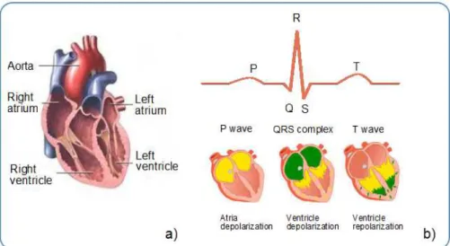
The electrocardiogram (ECG) is the recording, on the body surface, of the electrical activity
generated by the heart. The heart muscle has four chambers; the two upper chambers are called the atria, and the two lower chambers are called the ventricles (Figure 2.3 a)). Located
in the top right atrium there are a group of cells that act as the primary pacemaker of the heart [6]. Via a complex transformation of ion concentration in the membranes of those cells
event [8]. Because the body acts as a pure resistive medium, these potential fields extends to
the body surface.
The ECG wave results from the electrical measure of the sum of the ionic changes within
the heart. The observed waveform in the surface depends on the stimulated tissue mass and the current velocity [8]. A standard ECG pattern consists of a P wave, a QRS complex and
a T wave (Figure 2.3 b)). P wave represents the atria depolarization and QRS complex is assigned to depolarization of the ventricles. Ventricular repolarization shows up as the T
wave, while atrial repolarization is masked by ventricular depolarization [7].
A great research field within biomedical engineering is concerned about developing
me-thods for acquiring and analysing ECG signals. Changes in the amplitude and duration of the ECG pattern provide useful diagnostic information. The length of time between QRS
complexes also changes over time as a result of heart rate variability (HRV), also used as a diagnostic tool.
Figure 2.3: ECG signal principles: a) heart chambers b) ECG waveshape physiologic origin. Adapted from [10]
Force
Force is measured in a wide range of biomedical engineering activities, including gait analysis,
implant development and testing, material property measurement, clinical diagnosis, and the study of structure and functional relationships in living tissue [8].
A common form of force sensor is the load cell. Apply a force to the load cell stresses its material, resulting in a strain that can be measured with a strain gauge. The strain is then
pressure) and the vertical ground reaction torque are usually measured with force platforms
embedded in the walkway [6]. A force platform is a rectangular metal plate with piezoelectric or strain gauges transducers attached at each corner to give an electrical output that is
proportional to the force on the plate [11]. It can be useful when training stability of olympic shooters before pulling the trigger or training gymnasts during floor exercises by allowing
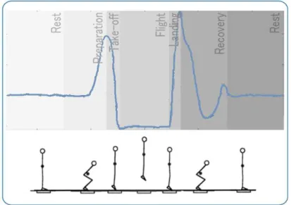
the continuous monitoring of the center of pressure displacement below the feet [3]. In the context of strength and power assessment it is mainly applied to evaluate the performance of
vertical jumps by athletes while standing on it (Figure 2.4), since jumping is generally used as a method of evaluation of reactive and explosive force in lower members [1].
Figure 2.4: Illustration of the signal acquired from a force platform during the several phases of a counter-movement jump. Adapted from [12] and [11].
Accelerometry
Acceleration is the rate of change of either the magnitude or the direction of the velocity of an
object, and it is measured in units of length per time squared (i.e., m/s2) or units of gravity (g) (1 g = 9.81 m/s2) [8]. Multiaxis accelerometers can be employed to measure both linear
and angular accelerations (if multiple transducers are properly configured). Accelerometers are currently available with up to three orthogonal measurement axis (Figure 2.5). Velocity
and position data may then be derived through numerical integration, although care must be taken with respect to the selection of initial conditions and the handling of gravitational
effects. A three-dimensional (3D) accelerometer can also provide inclination information when not accelerated and, therefore, only sense gravity [4]. In that case, its sensitive axis
sensitive axis at a known angle relative to vertical and measuring the output [8].
Accelerometers are used in a wide range of biomedical applications. In motion analy-sis, e.g., lightweight accelerometers and recording devices can be worn by patients to study
activity patterns and determine the effects of disease or treatments on patient activity [6]. Accelerometers are also widely applied on wearable systems for biomechanical analysis and
assessment of physical activity. Being directly applied on the body segment to be monitored, those systems are also able to match the requirements of portability and user comfort in
athle-tic performance evaluation usually not covered by the standard motion analysis instruments, such as force platforms [4, 13].
Figure 2.5: Acceleration signals acquired from the three axis components (x,y,z). The mean accelera-tion curve is computed by averaging the signal from each component. From [14].
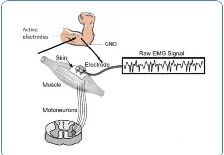
Electromyography
Electromyography (EMG) signal arises from the flow of charged particles (ions) across the muscle membrane when its cells are electrically or neurologically activated. A set of muscle
fibers innervated by the same motorneuron is defined as a motor unit. When a motor unit is recruited by the brain, the impulse (called action potential) goes through the motorneuron
and to the muscle (Figure 2.6). EMG signal is typically obtained by measuring the action potentials from multiple motor units. The signal can be acquired either by fine wires inserted
into muscle (intramuscular) or electrodes placed on the skin´s surface (surface EMG, sEMG) [6, 8]. In this dissertation the considered EMG signals were acquired by surface electrodes,
even if not specifically referred as sEMG signals.
Data collection variables that affect the quality of EMG signal are the placement and the
Being an electrical recording of electrical activity in skeletal muscles, the EMG is generally
used for the diagnosis of muscular disorders. Several authors have done a survey dealing with the relationship between the EMG signal and the related strength, coming to the conclusion
that the root mean square (RMS) value of this signal has a close relationship with the exerted muscle strength [8]. Furthermore, it is possible to check the existence of exerted
muscle strength and fatigue in frequency domain, e.g., with associated shifts for the median frequency in the EMG Power Spectral Density (PSD) [8, 15, 16].
Figure 2.6: Surface EMG: after the action potential goes through the motorneuron and the muscle, it is collected by active electrodes at the skin’s surface. A ground electrode is also necessary. Adapted from [17].
2.1.5 Statistical Concepts
Through this dissertation it is made reference to some statistical concepts that are standard when characterizing discrete-time signals. Following some brief definitions for those concepts
are presented.
Considering a signal defined over a finite time window with lengthN and represented as
time series [x(n)], its mean (or expected value) corresponds to the average of all the values of that series [5]:
µ= 1
N N−1
X
n=0
x(n) (2.4)
The variance is used as a measure of how much the signal values are spread out from each other. It is computed as the average squared deviation of each value from the mean of the finite signal:
σ2= 1
N N−1
X
n=0
The standard deviation(STD) is the most commonly used measure of spread and it is defined as the square root of the variance.
A possible approach when trying to model a deterministic signal as a time dependent
function is to use alinear regression, generally expressed by:
ˆ
x(n) =αn+β (2.6)
where αand β, the regression parameters, are computed in order to minimize themean squared error (MSE), a value that quantify the difference between the values implied by the linear regression and the true values of the original signal:
M SE= 1
N N−1
X
n=0
[x(n)−xˆ(n)]2 (2.7)
When modeling deterministic biosignals the use of a linear regression is restrictive. There-fore, apolynomial regression, by which the signal is modeled as a nth order polynomial,
may be a more accurate method of fitting a mathematical function to a time series data.
2.1.6 Synthetic Signals
Beyond being applied to the aforementioned biosignals, the tools developed in the context
of this dissertation were also applied to synthetic signals, as part of the algorithm perfor-mance evaluation methodology. This sub-section presents the general mathematical
forma-lism followed while defining those signals.
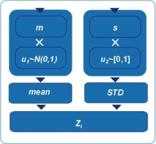
Synthetic signals are constructed by concatenating sections with predefined mean and
STD values (referenced as zones, Zi). In Figure 2.7 a block diagram outlining that
cons-truction process is presented. The mean values are given by float numbers, u1, randomly sampled from a standard normal distribution and then multiplied by a factor m. The STD
values are obtained by multiplying a random number u2, sampled from a uniform distribu-tion, within the interval [0,1] by a factor s.
Between those zones, transition events with known, randomly selected starting and ending points are also considered. Minimal values for mean and STD differences between
successive zones are imposed and assigned to them dand sd dvariables, respectively. Thus, a new zoneZi is rejected unless the following condition is verified:
mean(Zi)−mean(Zi−1) ≥m d
^
ST D(Zi)−ST D(Zi−1)
≥sd d (2.8)
seg-Figure 2.7: Blocks diagram describing the construction steps of a new zone to include in a synthetic signal.
mented into slices (Zij) with 10% of the its length. Then, it is assured that mean and STD differences equal or bigger thanm dandsd d, respectively, are not verified between successive
slices within a zone:
mean(Z
j
i)−mean(Z j−1
i )
≤m d
^
ST D(Z
j
i)−ST D(Z j−1
i )
≤sd d (2.9)
Otherwise, the new zone is rejected. Depending oh the chosen m d and sd dparameters
values, the aforementioned restrictions allow the successive zones of synthetic signals to be, or not, clearly distinct in terms of mean and STD values, without much variability of those
parameters within each of the individual zones.
2.2
Events Detection and Signals Segmentation
Automated techniques for generating, collecting and storing data from scientific measure-ments have become increasingly precise and powerful. However, there is still a practical need
to improve forms of data-mining, allowing the detection of specific events, the extraction of signals patterns, or even for distilling the scientific data into knowledge in the form of
analytical natural laws [18].
The implementation of biosignal pattern recognition and interpretation systems must
in-clude the extraction of signal features (as structural characteristics or transforms) that are important to pattern classification [19]. Those can then be used either for comparison with
stored data (allowing pattern detection, discrimination or classification) or for estimation of pattern parameters [19]. Since a large amount of data can be generated when considering
this end when applied to data compression algorithms [19].
An usual approach to recognition-oriented signal processing consists of using an auto-matic signal segmentation as the first processing step. This process can be described as the
automatic segmentation of a given signal into stationary (or weakly nonstationary) segments, which length is adapted considering the local properties of the signal [21] and the analysis
scale that is considered. The main goals are therefore the detection of the changes into the local characteristics, the estimation of the time points where the changes occur [21], and
most of all have the ability to automatically distinguish between meaningful and insignificant changes.
2.2.1 Signal Events
An event is broadly defined as the change in state of the system under study [19]. After
that the events are well marked on a signal representation of the system state, the respective patterns can be accessed by infering either the structure (a deterministic characterization of
signal form, e.g. geometric and angular relationships) or the trend (the way in which a specific type of structure, expressed as the magnitude of the respective reference variables, changes
in space or time) [19,22]. In the biosignals context the events could be e.g. heartbeats, EMG activations or even particular directed thoughts, for brain-computer interfaces (BCI) [23].
Despite the fact that pattern analysis problems in general, and the events detection in particular, become trivial under carefully controlled conditions, in practise that is not usually
verified [19]. Biosignals are often nonstationary, being characterized by oscillations at specific frequencies, and contaminated byin-band noise, which is both periodical and stochastic [24].
These issues are particularly important when considering the application of these algorithms in signals acquired from portable devices: the artifacts caused by increased movement and the
requirements for unobtrusive measurements causes the signal quality to be reduced compared to that achieved when performing measures in a laboratory environment [25]. Furthermore,
there are many types of events (and we may be only interested in some of them) and the relationship between the actual event and the signal resulting from it may be quite complex,
and often partially characterized.
Finding events in noisy signals is considered as a fundamental task throughout physics
and particularly the biosignals analysis research field [23]. The main desired properties of an events detection and signal segmentation algorithm are few false positives and missed
should be able to mark clealry the change points (the determination of signal activation
onset and the general transients detection) are presented. Some of the respective standard detection algorithms are also reported.
Onset
The accurate biosignals onset determination is useful in several studies of motor control and
performance. It is widely applied on neurosciences studies with kinematic data analysis, allowing the extraction of several parameters such as the reaction time or the peak velocity
time. Single-threshold velocity or acceleration methods are usually applied [26, 27]. These are, however, very sensitive to weak and abnormal response profiles, typical of some central
motor disorders, introducing variability and systematic errors into the results. As such, more accurate onset detection methods have been proposed.
Gerhard Staude [26] introduced a model-based algorithm that comprises an adaptive whitening filtering step followed by a Log-Likelihood-Ratio test to decide whether a
signifi-cant change occurred and estimate the change time. Despite the accuracy of this method and the possibility of improving its results by including a priori knowledge on the
physio-logical background of the measured signals, it requires extensive modeling and computation. Less complex approaches have been developed, e.g. the onset detection method proposed by
Botzen et al. [27]. This method employs a deterministic motor control model and a linear regression to estimate the change-point between a static and a movement phase, both of
which are assumed to be corrupted by normal zero mean Gaussian noise.
When considering applications such as neurological diagnosis, neuromuscular and
psycho-motor research, sports medicine, prosthetics or rehabilitation it may also be important to measure the time difference between the muscle activation and the movement onset [27].
Furthermore, in order to allow comparisons between different muscles, experimental condi-tions and subjects, the accuracy of burst onset, duration and offset determination for EMG
activity is crucial [28].
A comparative study regarding several methods for EMG signals onset detection is
re-ported by Staude et. al [29]. The basic processing stages of all the analysed standard detection methods, for which a blocks diagram is represented in Figure 2.8, are:
• Signal conditioning: applied to reduce the high frequency noise;
• Detection unit: comprises a test function (g[k]) computed from the pre-conditioned
signal and a decision rule. For each signal sample, Xk, the test function uses an
the decision rule (which compares it with a specific threshold h) to determine when a
change in the muscle activation pattern occurred;
• Post-processor: estimates the exact change time ( ˆt0) after that an event alarm (ta) has
been given by the detection unit processing stage.
Figure 2.8: Typical onset detection scheme. Adapted from [30].
Apart from the intuitive but error-prone visual inspection, the simpler computational
method approached by that study is the threshold-based Hodges detector [28]. After applying a lowpass filter to the rectified EMG wave, this algorithm computes the point where the mean
of N signal samples exceeds the baseline activity level (the signal average value considering a samples segment prior to stimulus) by a specific number of standard deviations. As well as
for other simple threshold-based methods, their results are highly dependent on the selected parameters ( particularly the threshold level and the lowpass filter cutoff frequency). As
such, Hodges detector is particularly suited to apply in high SNR conditions [29].
In conditions of low SNR the use of an adaptive pre-whitening filter, as proposed by
Bonato [31], proved to be superior than a less specific lowpass filter [29]. Other model-based approaches based on statistically optimal decision rules are also compared. Despite their
bigger accuracy, those methods depend on the a priori knowledge (or estimation) about the variance profiles before and after the change to be detected, being more complex and
time-consuming than the previously referred algorithms [29].
Transients
Signal transients can be considered as a wider events class which are characterized by a
sudden change into signal properties, such as the amplitude or the frequency, and with a short duration if compared to the observation interval [32].
Very important measurement information is often associated with the transients [33]. Abrupt changes or discontinuities encountered in biosignals may be symptomatic of
which corrupt the waveform to be analysed. In order to carry out an accurate measurement
of the waveform and to identify probable sources and causes for those transients, they should be detected and also measured in terms of significant parameters such as duration and
am-plitude, possibly in very low SNR conditions [33].
Given their relatively short duration (considering all the signal observation interval),
tran-sients influence into the signal spectrum is limited [34]. Therefore, the standard methods for transients detection are mainly based on time-frequency analysis with the use of theWavelet
transform [32, 36]. The Continuous wavelet transform assures a good time resoultion that allows the evaluation of transients arrival times and their duration; the disembodying of
the transient from the global waveform, for posterior parameters extraction, is achieved by performing a proper decomposition and a subsequent reconstruction of the original signal in
frequency subbands by means of the Discrete time wavelet transform [32].
The present research work followed an alternative approach, by identifying time domain
specific morphological parameters that can clearly distinguish those events from the complete observed signals. This chapter presented the base concepts that will be used in the following
Events Detection Algorithm
In this chapter the events detection algorithm developed in the context of this dissertation is presented. The first section approaches the adopted mathematical formalism and the
processing steps concerning its implementation are presented in section 3.2. Section 3.3 introduces the events detection algorithm real-time implementation approach.
3.1
Mathematical Formalism
3.1.1 Events and Signal Modeling
For a given signal defined as a time series,x(t), witht= 1,2, ..., L, a set of regions is created
by slicing the signal. Considering E as the total number of events, a general event slicing signal regions is denoted by ei, i= 1,2, ..., E. According to the adopted notatione1 and eE
are, respectively, the first and the last events of the considered time series. The complete modeled signal is expressed as defined in equation 3.1, for which further notation is described
below:
ˆ
x(t) =
E−1 X
i=0 Q
t
ei+1−ei −ei
M(t−ei, Ai, ε) (3.1)
Q(t) is an unit pulse function expressed by:
Q(t) =
1 if 0≤t≤1
0 otherwise
(3.2)
Considering ei t
+1−ei as the argument of this function, the time interval in whichQ(t) = 1 corresponds to the signal segment length between those events. Subtractingei, that pulse is
M(t, A, ε) is a polynomial regression model defined by:
M(t, A, ε) =A(t) +ε (3.3)
where A is the matrix with n polynomial parameters for a given signal region A(t) =
a0 +a1t+a2t2 +....+antn and ε is an error term that is assumed to follow a normal
distribution ε=N(µ, σ2)
withµ= 0.
After modeling the signal as described above, each one of the E−1 signal segments can
be described as:
ˆ
xi(t) = ˆx(t)|t∈[ei,ei+1] (3.4)
3.1.2 Events Computation and Stopping Criteria
The set of events detected within a given signal are the result of an iterative process that
considers different stopping criteria in order to return an optimal solution:
• Maximal standard deviation gradient: this parameter is evaluated by computing
S, defined as the sum of the absolute standard deviation differences between successive segments ˆxi(t) within a signal:
S = E X i=1 std(ˆx
i(t))−std(ˆxi+1(t))
(3.5)
• Minimal MSE: the fitting quality of the applying model is also considered by com-puting D, defined as the sum of the mean squared error values through the successive regions (with lengthNi):
D=
E+1
X
i=1
PNi
t=0(xi(t)−xˆi(t))2 Ni
(3.6)
• Maximal number of events.
The optimal solution is achieved by varying a set of implementation parametersP, further described in Section 3.2.2. P parameters include the length of the signal slices from which
to compute a standard deviation difference sequence and a multiplying factor that affects the length of the moving average window considered in the smoothing filter to apply on the
Those parameters are then iteratively changed in order to fulfill the following condition:
ArgMin
P
[D−S−E] (3.7)
3.2
Implementation
The following sub-sections introduce the main processing steps implemented in order to
approach the mathematical formalism decribed in section 3.1. The algorithms were designed using Python programming language, with the Numpy [37] and the Scipy [38] packages.
3.2.1 Algorithm Design
The main goal of this algorithm is the signal segmentation into clearly distinct zones, by an
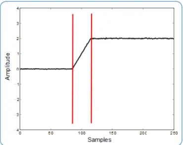
accurate estimation of the time points in which significant changes into signal local features occur, as exemplified in Figure 3.1.
Figure 3.1: Example of a synthetic signal with marked events.
Those changes are evaluated by quantifying the differences between the standard
devia-tion of successive regions within the signal. The sets of regions for which that differences are more pronounced are marked within the signal, being these marks called as notable points.
The events definition is then achieved by applying a more accurate evaluation within those regions.
specific preprocessing steps. Nevertheless, beyond the signal, it can receive other parameters,
by input, in order to run auxiliary functions (Table 3.1) responsible for each of the processing steps described below .
Table 3.1: get_events algorithm auxiliary functions
Function Input Output
get_slices_std signal STD sequence
slices length
adjust_peaks signal adjusted peaks
slices length
peaks peaks type
The auxiliary functions input parameters are given during the optimization phase
(des-cribed in section 3.2.2) and not directly by the user. Figure 3.2 shows a block diagram for
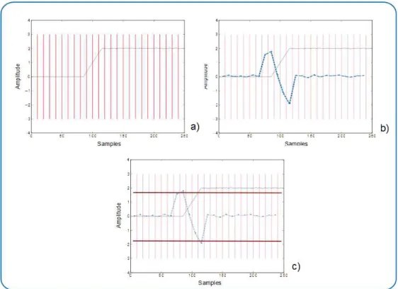
get_events algorithm, which integrates either the input and output parameters, as well as the referred auxiliary functions. In Figure 3.3 the first processing steps of this algorithm applied to the signal on Figure 3.1 are graphically represented.
Figure 3.2: get_events algorithm flowchart diagram. This algorithm receives the signal and the
slices length,smooth f actor and thepeaks f actorparameters as input. After slicing the signal, by applying theget_slices_stdauxiliary function, its notable points are computed. Theadjust_peaks
auxiliary function is then applied to compute the events and the signal regions between those points, returned by this algorithm.
Signal Morphological Analysis
From a raw signal, the get_slices_stdfunction divides the signal into slices with a defined
STD.
The signal morphological analysis follows by computing the first derivative of the standard deviation sequence previously defined. By analysing the resulting sequence (to select the
signal notable points, as following described) the developed algorithm is able to perform a preliminary identification of the signal regions where the greatest pattern variability is
verified.
The number of samples considered in each signal slice must always be bigger than 1. In
practise, however, the number of samples in each slice should be bigger to allow the algorithm to distinguish natural random fluctuations from symptomatic tendencies. By default, that
value is set to a minimum of 10 samples.
Figure 3.3: Illustration of the get_events algorithm first processing steps: a) Signal slicing; b) Smoothed STD sequence; c) Notable points selection.
Notable Points Selection
After the first derivative of the STD sequence is obtained, the resulting sequence is low-pass filtered. A smoothing filter, in which the number of points considered into the moving average
window depends on the length of the sequence multiplied by a specific input (smooth f actor) of this algorithm (Figure 3.3 b) ), is applied.
found above/below a specific threshold (Figure 3.3 c) ). The former is defined multiplying
the absolute sequence maximum/minimum by thepeaks f actorinput parameter (Figure 3.2).
Events Definition
After the preliminary signal notable points are computed, the adjust_peaks function is
applied to these points aiming at an accurate events detection within the slices from which those were selected. This function receives the signal, the peaks, the considered peaks type
(maximums or minimums) and theslices length as input. For each peak this function con-siders the signal slice beginning in that point and then applies theget_slices_stdalgorithm
on that signal segment (with a fixed slices lengthof 5 samples). If a maximum peak is con-sidered, it is then replaced by the point that maximizes the difference on the computed STD
sequence. For minimums the procedure is analogous. This processing step ensures a more accurate events detection, with a minimum error of 5 samples.
At the end, theget_eventsalgorithm returns the detected events and an array with the
successive signal regions between those events.
3.2.2 Optimization Process
An optimization algorithm was defined, based on a iterative computation of the signal events by applying the get_eventsalgorithm with a set of different input parameters. An optimal
solution is returned with the set of parameters for that the stopping criteria defined in section 3.1 are better fulfilled. This is accomplished by applying theget_opt_events algorithm, for
which a flowchart diagram is represented in Figure 3.4.
Parameters Range
Theslices length parameter range is defined by considering the signal length (L) and inclu-ding increasing values (raising by one unit) between mand M, defined as follows:
m=L/1000, ∀L≥104 :m≥10
M =m+L/100, ∀L:M ≤40
(3.8)
As previously described the number of samples in each signal slice must be significant to allow the algorithm to evaluate if a change into the morphology should be marked as an
Figure 3.4: get_opt_eventsalgorithm flowchart diagram. This algorithm performs the events detec-tion optimizadetec-tion process. Its input parameters are the signal and thescalefactor (optional). From those, slices length, smooth f actorand peaks f actor ranges are defined and theget_events algo-rithm is applied considering each combination of those input parameters. The solution that better fulfill the optimization criteria is then selected and returned by theget_opt_eventsalgorithm.
10.000 samplesm is set to 10. The upper limit is set to a maximum of 40 samples.
The following processing steps allow the algorithm to define the smooth f actor and the
peaks f actor parameters range to be considered into the iterative optimization process:
• The signal is normalized dividing each sample by the mean value of the considered
time series. From the resulting signal, for which the mean value is equal to 1, the standard deviation is computed and assigned to a specific variable (sm). By applying
the normalization procedure it is ensured that thesmvalue does not depend upon the signal offset and only express its variability;
• A scale factor is also defined dividing L by successive higher powers of 10 until a value
lower than 1 is reached. It can alternatively be given as an input, allowing the user to choose the level of detail, related to the minimum pattern discontinuity magnitude
that will turn it into a detected event;
i= smfi ×scale u=i+smfu ×scale
(3.9)
Both smooth f actorand peaks f actor ranges limits follow the formalism described in equation 3.9. The considered fi and fu for each range are presented in Table 3.2, as
well as the maximum values allowed for each limit.
• The step values are similarly defined for both the smooth f actor and peaks f actor
ranges by analysing their inner limit values. In each case, if i is lower or equal to 0.1
the range step is 0.05. Otherwise, a step of 0.1 is considered.
Table 3.2: Specific parameters forsmooth f actorandpeaks f actorranges.
Inner limit Upper limit
fi max fu max
smooth f actor 0.5 0.2 10 0.5
peaks f actor 1 0.2 10 0.5
The followed implementation approach performs the smooth f actor and peaks f actor
ranges shifting and expansion depending upon the scale factor and the global signal variability,
represented by its normalized standard deviation value (sm).
In general, the range values vary inversely with the sm values. For a given signal, when
a significant variability is verified in specific regions, rendering high sm values, the events detection is straightforward. As such, the moving average window to be considered when
applying the smoothing filter to extract the signal notable points should be relatively small to ensure the detection accuracy is not compromised. Likewise, and since those notable points
are clearly pronounced, the considered threshold levels when performing their selection are not to high, to avoid some possible missing detections.
In conditions of low sm values, the detection of significant pattern discontinuities may be more complex. Therefore, both the smoothing moving average window length and the
threshold levels previously described should raise to avoid a false positive events detection.
Optimization
When considering global optimization problems, iterative methods are usually applied. In
perhaps most natural optimization approach passes by evaluating all the parameters domain,
performing an exhaustive (or brute force) optimization. This method tests each potential solution, so the best combination of factors can be found [40, 41]. Following this exhaustive
search model, all the experiments are conducted before any judgment is made regarding the optimal solution [42].
Alternatively, some searching techniques follow a different approach, by which the opti-mization is made sequentially (each new choice for the best solution is gathered from the
preceding choices [39]). The Simulated Annealing [43, 44] and Step Size Algorithms [40] are examples of sequential optimization methods. Genetic algorithms, based on the mechanics
of natural selection and genetic, are also widely applied [40, 45].
In general, exhaustive optimization is relatively inefficient compared to sequential search
or genetic algorithms approaches, mostly because the time required to perform it is dramati-cally increased when the number of parameters increase [42, 45]. However, if the number and
domain of those parameters is finite and relatively small, an exhaustive search is a simpler and reasonable approach [40]. Therefore, that was the methodology adopted at the
optimiza-tion phase of the presented events detecoptimiza-tion algorithm.
For each set of parameters the get_events algorithm is applied. The results are then
selected, applying the optimization criteria defined in sub-section 3.1.2. Either the solutions that have the minimum total MSE, considering all the signal segments modeled as 1st order
polynomials, or the maximum total standard deviation differences between those segments
are selected in the same step. From those, the one for which the number of events is maximal is selected as the optimal solution.
3.3
Real-time Implementation
This section introduces a real-time signal processing application developed during this
re-search work. The standard real-time processing constraints and the adopted events detection algorithm implementation approach are also discussed.
3.3.1 Real-time Signal Processing Tool
This appliaction for real-time signal processing was built on a general-purpose and object-oriented programming basis. It was developed using Python programming language (version
In-terface (GUI), from matplotlib, together with the Antigrain drawing toolkit [50].
The signal acquisition is performed by bioPLUX research units [51]. The developed application uses a Python Application Programming Interface (API) available together with
the bioPLUX unit, in order to control whether the device is acquiring the data and obtaining the digital raw signals from its several channels. By allowing the acquisition from up to two
bioPLUX research units, this tool enables the data from sixteen independent sensor sources to be collected, visualized and processed in real-time. Both the raw and processed data can
also be saved in text files for post-processing.
The objected-oriented programming approach allows a clear distinction between
inde-pendent structural elements within the program, called as blocks. These are classes which may also use objects instantiated from other classes, in such a way that the blocks and the
respective parameters are easily configured by the user. The organization and the data flow between the several blocks are described in Figure 3.5. Following this architecture and a brief
description of the several structural blocks is reported.
Figure 3.5: Real-time processing application: blocks description and data flow.
Structural Blocks Description
Acquisition class allows the connection to the bioPLUX units (by applying the Python API proper commands), the beginning of the acquisition and the repetition of this process
at a user configurable rate. That rate defines the number of acquisition frames collected at a single time from the bioPLUX unit buffer, which are sequentially addressed to a specific
frame (or to the concatenation of the acquisition frames from two devices, if applicable). The
acquisition end is also applied by a specific method of this class.
If the data from two bioPLUX devices is acquired, this block also calls an auxiliary
Synchronism class. When the acquisition begins the main method of this class is able to find the time lag between the signals from both devices, by reading their digital port data
(previously set with the same output value by successive commands execution). This lag is eliminated by acquiring and discarding the same number of frames only from the delayed
device.
Visualization class is responsible for creating the GUI main window by instantiating an object from an auxiliary class (AnimatedPlot). The several subplots elements are then added in a predefined sorted way and the methods that perform the signal updated plot are also
called in this block.
When using a matplotlib GUI to build animated plots, the basic approach passes by
cre-ating a figure and a correspondent callback function that updates it, which is passed to the specific GUI idle handler or timer [49]. In this application the AnimatedLine class allows the
creation of the first lines to be plotted in each subplot element, defining the respective axis scales. This class includes also the necessary methods to update those lines with new data,
as well as designing animated vertical markers above those lines. Those methods are then applied by a function of the AnimatedPlot class.
An higher performance on signal plotting is achieved, when applying the specific Animated-Plot class method, by drawing a background and animating the necessary plot elements on
top of it in each updating loop, as proposed in [49]. By default, the signals are only partially updated by the same predefined amount of samples (the same as the acquisition rate), but
keeping a static background, in order to enable the visualization of its progress over time. It is also possible to obtain the visualization of the whole signal, updated at each loop, what
is useful, e.g., when representing the signal spectrum (computed by applying the specific Processing block method).
Either the subplots labeling (according to the bioPLUX number, as ordered by the user when configuring the application, and the respective channel number, as exemplified in
Fi-gure 3.6) and sorting are assigned to the visualization class. The subplots sorting is done according to the following rules:
• If some processing is also required by the user the result is plotted, by default, after
the correspondent raw signal position, whether the former is asked or not (Figure 3.6 b) and e) ).
• The results of algebraic operations between signals is an exception, being always plotted after all the raw and processed single channel data (Figure 3.6 f) ).
Figure 3.6: Real-time processing application GUI main window
Writing class allows the user to save the data acquired from the bioPLUX devices into a text file, so it can be post-processed. The data is presented in a column format. Each
column contains the data from one of the selected channels. The order the data from the several channels is placed, as well as the information about from what bioPLUX device it
belongs is explicit into the file header.
If some processing is required by the user the processed data is also written, by default,
in successive columns after those that contain the raw data. The correspondence between each column and information about from what channel that processed data was originally
acquired and what type of processing was performed is also provided in the header part of the file.
Processing the acquired data in real-time is the main feature of the developed applica-tion. Since the basic processing is done directly over the acquisition frames available at each
updating loop, it is ensured no time lag between the raw and processed visualized data. After the acquisition block returns the tuple containing the several acquisition frames, the
![Figure 2.1: Biosignals classification according to the signal characteristics. Adapted from [6].](https://thumb-eu.123doks.com/thumbv2/123dok_br/16540230.736693/27.892.128.788.115.571/figure-biosignals-classification-according-signal-characteristics-adapted.webp)